Buffering and flow control in message switched communication networks by Eberhard Frank Wunderlich.

January, 1978 Report ESL-R-797

BUFFERING AND FLOW CONTROL IN MESSAGE SWITCHED COMMUNICATION NETWORKS

by

Eberhard Frank Wunderlich

This report is based on the unaltered thesis of Eberhard Frank Wunderlich submitted in partial fulfillment of the requirements for the degree of Doctor of Philosophy at the Massachusetts Institute of Technology in January, 1978. This research was conducted at the Decision and Control Sciences Group of the M.I.T. Electronic Systems Laboratory, with partial support extended by the Advanced Research Projects Agency under Contract ONR/N00014-75-C-1183.

Electronic Systems Laboratory _Department of Electrical Engineering

and Computer Science

Massachusetts Institute of Technology Cambridge, Massachusetts 02139

BUFFERING AND FLOW CONTROL IN MESSAGE SWITCHED COMMUNICATION NETWORKS

by

EBERHARD FRANK WUNMDERLICH

B.S.E.E., University of Nebiaska-Lincoln (1974)

S.M.E.E., Massachusetts Institute of Technology (1975)

SUBMITTED IN PARTIAL FULFILLMENT OF THE REQUIREMENTS FOR THE

DEGREE OF

DOCTOR OF PHILOSOPHY at the

MASSACHUSETTS INSTITUTE OF TECHNOLOGY (January 1978)

Signature of Author ... Department of Electrical Engineering and Computer Science

January 11, 1978

Certified by ... ... Thesis Supervisor

Accepted by ... ... ...

BUFFERING AND FLOW CONTROL IN MESSAGE SWITCHED COMMUNICATION NETWORKS

by

EBERHARD FRANK WUNDERLICH

Submitted to the Department of Electrical Engineering and

Computer Science on January 11, 1978 in partial fulfillment

of the requirements for the Degree of Doctor of Philosophy.

ABSTRACT

This mathematical study of buffering and flow control is based on a gradual input queueing model. The gradual input model has been used previously to study data multiplexors.

Here it is extended to an entire message switched

communica-tion network.

A probability of buffer overflow analysis is developed

and used to determine buffer requirements. A delay analysis

is also developed. The results obtained using the gradual input queue are compared to the commonly used i/M/l queue model for message switched networks. The gradual input model

allows one to observe several effects due to a finite number of finite rate traffic sources in such networks that cannot be observed using the M/M/1 model.

Flow control is studied in tree concentration structures. The flow control assures that buffer overflows will occur

only at source nodes, not in the interior of the tree. The problem of finding the buffer allocation that minimizes the probability of buffer overflow in such a tree is studied. It is shown that in certain cases it is optimal to place all buffers at source nodes. This is, however, not always so and insight into this is given by example.

Determining the performance of a tree structure in which flow control is bieing used is a difficult analytic problem. An approximate analysis based on a first passage time theorem for Markov chains is therefore developed for an example.

The approximate analysis is verified by simulation.

Thesis Supervisor: John M. Wozencraft

Title: Professor of Electrical Engineering 2

ACKNOWLEDGEMENTS

I gratefully acknowledge the assistance of my thesis supervisor, Professor John M. Wozencraft. His guidance and advice have been most helpful during the course of my thesis research and throughout my graduate studies at M.I.T. It has been a pleasure to work with him.

I am thankful to my thesis readers, Professor Robert G. Gallager and Professor Nils R. Sandell, Jr. for their

comments. Several of their suggestions led directly to results contained in this thesis.

I would also like to acknowledge assistance from

Dr. Pierre Humblet, Dr. Joe Defenderfer, Dr. Ronald Pannatoni and Dr. Loren Platzman. They reviewed many of my ideas and contributed to them. Dr. Humblet was especially helpful in adding mathematical insight to this study.

The thesis was skillfully typed by Ms. Sandy Margeson. This study was done with support from a Vinton Hayes Fellow-ship and by the Advanced Research Projects Agency under

Contract ONR/N00014-75-C-1183.

I would like to thank my parents for their support and encouragement throughout my student years. Finally, I thank my dear Shahla who has filled my life with joy while I was completing this thesis.

TABLE OF CONTENTS Page TITLE PAGE. ... .. 1 ABSTRACT. ... . ... 2 ACKNOWLEDGEMENTS . . . 3 TABLE OF CONTENTS ... 4 CHAPTER I -INTRODUCTION ... .... 6

1.1 Description of the Problem . ... 6

1.2 Previous Studies of Buffering and Flow Control. . ... 12

1.3 Sun-mary of Results ... . 19

CHAPTER II- THE ANALYSIS OF A SINGLE GRADUAL INPUT QUEUE ... .... . .... . 23

2.1 The Basic Gradual Input Queue Model . 23 2.1.1 Definitions and previous results . . . 23

2.1.2 Equivalent M/G/1 queue service time analysis ... . . . 32

2.1.3 Bounds for the expected delay per bit . . . 45

2.2 The Gradual Input Queue With a Finite Buffer .. . . . .. 49

2.2.1 Probability of buffer overflow in a busy period. . .. . 49

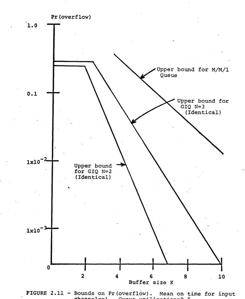
2.2.2 Examples of the bounds on Pr(overflow) . . . 54

2.2.3 A per unit time overflow measure .. . . . .... 63

2.2.4 Other overflow measures ? .. 72

2.3 Comparison of the Gradual Input Queue and the M/M/1 Queue . . .. 78

CHAPTER III-NETWORKS OF GRADUAL INPUT QUEUES. . . . . 86

3.1 Approximations for the Analysis of a General Network . .. . . 86

- 3.1.1 Traffic streams in general networks. . . . 8

3.1.2 Expected on-time for a

switched busy period . . . . 95 3.1.3 Determining the mean traffic

parameters in a general

network .. . . . 98

3.1.4 Simulation verification . . ..108

3.2 Examples of General Networks . . . .115

3.3 The Static Routing Problem . . . . .129

CHAPTER IV- FLOW CONTROL IN TREE CONCENTRATION

STRUCTURES . . . .. .137

4.1 Dete:mining the Optimum Buffer

Allocation in a Tree Concentration

Structure . . . .138 4.1.1 The optimality of buffering

only at source nodes. . . . .138 4.1.2 Flow control when all buffers

are at source nodes . . . .154 4.1.3 The effect of gradual inputs. .157 4.2 The Queueing Analysis of a

Concentration Tree . . . .171 4.2.1 An approximate analysis of

a two level tree. .. . . . .171 4.2.2 An example and simulation

verification . . . .186 CHAPTER V - CONCLUSION AND SUGGESTIONS FOR FURTHER

RESEARCH . . . ... . .189

5.1 Conclusion. . . . .189 5.2 Suggestions for Further Research . .193

APPENDIX A- RESULTS FOR THE GRADUAL INPUT QUEUE

WITH NONIDENTICAL INPUT CHANNELS . . . .195 APPENDIX B- A LIMIT THEOREM FOR FIRST PASSAGE

TIME DISTRIBUTIONS . . . .199

CHAPTER I - INTRODUCTION

1.1 Description of the Problem

Message switched communication networks are moving quickly into prominence as effective networks for data communication. Much of the current interest in message switched networks has resulted from the experience of the Advanced Research Projects Agency Network (ARPANET).

ARPANET demonstrated that a message switched network in which messages are sent as one or more packets can be an appropriate design choice for providing communications for computers [RBRTS 70, KAHN 72]. There are also a number of other packet switched networks which currently exist or are under development. These include the Cyclade Network

[POUZ 74], the Transpac Network [DANET 76], the commercial network Telenet and the military network Autodin [ROSN 73].

An important characteristic of message switched networks for data communication is that they can contain buffers.

Buffers allow the network to accept temporarily traffic from sources at a rate greater than the rate at which it is being delivered to the destinations. Since buffers have finite capacity, message switched networks require. flow control mechanisms to control the traffic sources in order to

prevent buffer overflow and other congestion problems (such as lock up problems or unacceptably high delay).

This study deals with the mathematical modeling and analysis of such buffering and flow control in message

switched networks. The work presented here consists of two major parts.

1) A gradual input queue model is developed and used to investigate the theoretical buffer requirements of a class of message switched networks.

2) The problem of optimal buffer allocation and flow control is investigated for tree concentration structures within such networks.

The message switched networks considered in this study are of the general type shown in Figure 1.1. The networks consist of sources and destinations interconnected by

directed communication channels through buffered message switching nodes. Some of the nodes are connected in con-centrating tree structures. The tree structures are then

interconnected with each other by a network whose structure is not restricted. In this general class of network

structures, the trees are the "local distribution" part of the network while the network interconnecting the trees is the "long distance" network. Since tree structures are less difficult to analyze than general networks, particular

emphasis is placed on them in this study. They are the only structures in which flow control is studied. This emphasis is also supported by the fact that the "local

distribution" costs are a very significant part of the total cost of a message switched network.

CT CT CT GENERAL INTERCONNECTION NETWORK CONCENTRATION TREE STRUCTURE (CT)

Message Switching Node

- .b- M - Directed Communication Channel

FIGURE 1.1 - General class of message switched networks studied

An enlarged view of a message switching node is shown in Figure 1.2a. Traffic arrives at a node over input

channels as an on/off process. The rate of arrival of the individual bits in a message is determined by the input channel capacity or source rate and messages arrive in a gradual, flow like manner. The switch sends messages to the correct output channel according to a fixed routing policy. The switch is assumed to operate instantaneously and in a continuous flow fashion. The continuous flow through the switch means that if there is no contention for an output channel, there will be no delay in passing through a node. Thus the node does not operate in a store and forward manner, in which a complete message must be received at a node before any of it is sent on the output channel.

The model thus can be used to obtain the theoretical buffer requirements due only to contention for communication channels of finite capacity (i.e. those buffer requirements not due to the nature of store and forward operation, finite

switching rates, or the need to store messages until error detection/retransmission or error correction is complete.) While this study deals with a flow-through network, many of

the insights obtained are applicable to store and forward networks as well.

The study assumes that buffers in the nodes are associated with only one output channel. This is not as efficient as one shared buffer pool for all output lines, but serves to make

Input Channels Output Channels

on on Buffers

L

Switch

a. Message switching node structure.

Inputs

Buffer Output

b. Input and output traffic for each buffer.

FIGURE 1.2 - Buffering in a message switched node

the mathematical analysis feasible. The division of buffer capacity in a node can also be supported by the fact that in actual systems, each output channel might have a dedicated communications processor with its own buffer.

As a result of the assumed buffer division and switch operation, each buffer is as shown in Figure 1.2b. Each buffer is fed by several input channels with on/off traffic and this produces in turn an on/off traffic pattern on the

output channel. The stochastic model of this buffer is

called a gradual input aueue. It has been studied by Cohen,

Rubinovitch and Kaspi [COHEN 74, RUBIN 73, KASPI 75] and it

is the basic model that is used in this study.

Previously, the gradual input queue model has been analyzed for networks of converging tree structures with infinite buffers at each node. The first major part of this study extends this model to general networks using a fixed routing policy for messages and no blocking or flow control between nodes. The extension also includes overflow measures such as a probability of overflow for finite

buffers in such networks.

In a message. switched network it is desirable to have flow control measures that can relieve congestion at a communication channel by reducing the rate of inflow to that channel. To analyze even simple flow control policies for general networks is extremely difficult. Therefore,

this study considers flow control only in converging tree structures. The second major part of this study-investigates the optimal buffer allocation and flow control for such

structures. The flow control considered involves flow rules that do not allow buffer overflows in the interior of the tree structure. Therefore, all overflows occur at source nodes where it would presumably be straightforward to turn off sources to avoid lost traffic.

In recent years there has been considerable interest in the analysis of message switched networks, flow control and related queueing problems. A survey of previous studies in these areas, discussed from the viewpoint of their relation to this study, is given in the next section.

1.2 Previous Studies of Bufferina and Flow Control

An early analytic study of the queueing processes that occur in the buffers of message switched communication net-works was done by Kleinrock [KLEIN 64]. Kleinrock modeled buffered communication channels as exponential service time

(message transmission time) queues with Poisson input streams of messages and infinite buffers (i.e. M/M/1 queues). A

communication network is then represented by a network of such queues. On the basis of the result that the output process of an M/M/1 queue is Poisson [BURKE 56], Kleinrock

argued that each queue in the network could be analyzed by merely determining the mean arrival rate into it. Each

queue in the network behaves the same as a single M/M/1 queue not in a network. This has been formalized by Jackson [JACK

57]. Jackson showed that for certain networks of queues, the steady state joint distribution for the number of customers at each queue has a product form. Each term in the product is the same as the distribution for an independent queue with the appropriate mean arrival rate. Using the network of

queues model, Kleinrzck considered a number of network

design problems, including finding the communication channel capacity allocation which minimizes the expected delay

through the network subject to a total network cost constraint. While buffer occupancy statistics were not explicitly

con-sidered in this study, it is straight forward to obtain the steady state results using the network of queues model.

It is important to examine the assumptions that were required to make the network of queues model mathematically

tractable. The main assumption is that if a message passes through more than one communication channel, its length

(service time) is chosen independently at each queue- (channel) through which it passes. This independence assumption is

necessary to remove the statistical dependence between the interarrival times and message lengths of adjacent messages in the network. A second assumption is that at the time of a message arrival, all of the information bits associated with that message arrive instantaneously at the channel

buffer. Clearly, if the communication channels have fi-ite 13

capacity, the information bits arrive gradually, not

instantaneously. The gradual input queueing models to be used in this study do not use either of these assumptions. Some assumptions will have to be made, however, for the gradual input model as well and they have some relation to the independence assumption used by Kleinrock. In particular, the gradual input queue analysis requires that the statistics of all input channels be independent. If in a general net-work, traffic with a common destination is routed over two

paths that share some channels, separate and then again share some channels, this will require a type of independence

assumption. The independence assumption is, however, not made for directly adjacent nodes.

A network of queues model has recently been used by Lam [LAM 76] to study the buffer requirements in a packet

switched network when each node of the network has only a finite storage capacity. The network is assumed to operate on a store and forward basis with link by link acknowledge-ment of messages. Using basically the same assumptions as Kleinrock in a more complex model, Lam obtains approximate results for the probability of nodal blocking due to buffer overflow. The study also develops a heuristic algorithm for determining a balanced assignment of buffer capacities in the network.

Another study of the queueing processes in networks of finite length queues representing message switched communica-tion networks has been done by Borgonovo and Fratta [BORG 73]. This study approached the problem by using an exact Markovian

state space model to represent the dynamic operation of the network. Such a model is feasible only for very small net-works with few buffers because the size of the state space grows extremely rapidly as the size of the network increases.

To overcome this problem, heuristic upper and lower bounds were developed for the probability of nodal blocking due to buffer overflow for symmetric ring networks. Borgonovo and Fratta overcame the independence assumption by working in discrete time with fixed length messages.

In addition to the above studies of complete networks, there have been numerous studies of the queueing processes associated with just one communication channel or one node of a message switched network [HSU 73, HSU 74, PACK 74, CHU 70A, CHU 70B, GORD 70, RUDIN 70, CHU 73, RICH 75, CHU 69, IRLND 75, WYNER 74]. Most of the studies assume that messages arrive as a Poisson process in an instantaneous manner. A study which does not make this assumption has been done by Gordon,

Meltzer and Pilc [GORD 70]. This study investigates the operation of a statistical multiplexor for message switched traffic that comes from a finite number of two state 'Markov sources by simulation. The sources are either in the on

state or in the off state and in the on state they generate a steady stream of characters at a finite rate. This is

much like the source model that will be used in this study of the gradual input queue. The Gordon study gives the buffer capacities needed to meet certain probability of buffer overflow requirements. The average character delay through the buffer was also obtained.

Flow control in a message switched network designed for computer-communication became a topic of interest during the design and subsequent operation of the ARPANET. The flow control mechanisms used in the ARPANET are discussed by

Kahn and Crowther [KAHN 72]. Two basic mechanisms are used, one for source to destination flow control and one for node to node flow control.

The source to destination flow control is achieved by defining a link to be a unidirectional logical connection between users of the network and then controlling the number of messages outstanding on a link at any one time. In

ARPANET, the rule used is that there can be only one message outstanding on a link at a time. This rule is enforced by sending a "request for next message" (RFNM) from the destina-tion to the source after each message is.received. The

source does not send the next message until it receives the RFNM.

The node to node flow control in ARPANET is based on a system of acknowledgement messages (ACKS). After a node sends a message to the next node, it keeps a copy of the message until it receives an ACK for that message from the

receiving node. Therefore, if the receiving node has no buffer space available, it can simply discard an incoming message and not send an ACK for that message. Then, after waiting a specified length of time and not receiving an ACK,

the sending node will retransmit the message.

Both the source to destination and the node to node flow control serve to effectively control congestion in many

circumstances. In some situations, however, these mechanisms can lead to lockup conditions or otherwise reduce network throughput. The avoidance of such lockup conditions and reduced throughput has led to modification of the specific flow control rules for ARPANET.- The basic concepts still apply, however.

There is only a limited amount of theoretical literature on flow control. One scheme that has been proposed and

analyzed to some extent is isarithmic flow control. Isarith-mic flow control was first described by Davies [DAY 72]. The basic idea is to have a fixed number of message carriers that are used to send messages through the network. An input

message must wait for a carrier to be available at the input

node before it can progress through the network. When a

carrier is empty, it circulates at random through the network until it arrives at a node that has traffic for it.

The main parameter associated with isarithmic flow control is the number of message carriers in the network. Davies has shown by simulation that throughput is a function of the number of carriers. If there are too few carriers, traffic is needlessl rejected at the inputs, while if there are too many carriers, congestion occurs. Davies points out that isarithmic flow control is not designed to completely replace other flow control mechanisms. In addition to the simulation study, Sencer [SENCER 74] has developed an analytic queueing model for isarithmic flow control.

The analytic evaluation of flow control mechanisms is in general very difficult. Recognizing this, Chou and Gerla

[CHOU 75] have proposed a framework in which to classify and then develop simulation models for such mechanisms. Their scheme, called the unified flow control model, recognizes that messages are allowed to enter a network or proceed through it only if 1) in some sense the buffers required have been allocated at the point of entry and/or if 2) the number of occupied buffers is below some threshold. Various flow control mechanisms differ in the rules for allocation and in the thresholds that are defined. Once these rules have been identified for a given mechanism, it can be

Some reference to a flow control scheme that is similar to the rate flow control consider in this study has been made in a survey by Gerla and Chou [GERLA 74]. The survey mentions a proposed flow control strategy due to Pouzin

that controls input rates on the basis of the information in flow control tables which are circulated in the network. The flow control considered in this study also controls flow rates. Extensive flow control tables are, however, not needed in this study since it is limited to concentration tree structures. In such structures flow control can consist of simply reducing the flow rate of upstream nodes whenever downstream nodes

become congested. The flow control problem for a general network is much more complicated and Pouzin ha., apparently not analyzed his proposed scheme mathematically.

1.3 Summary of Results

A single gradual input queue is first considered in detail since it is the basis of this study. Chapter 2 presents the previously known results for this model and a number of extensions. An important extension required for this study is a probability of overflow measure for a queue with a finite buffer. The probability of overflow per busy period is found and a useful exponential upper bound for it is also obtained. It is shown how this overflow measure can be converted to an expected time between overflows. Other

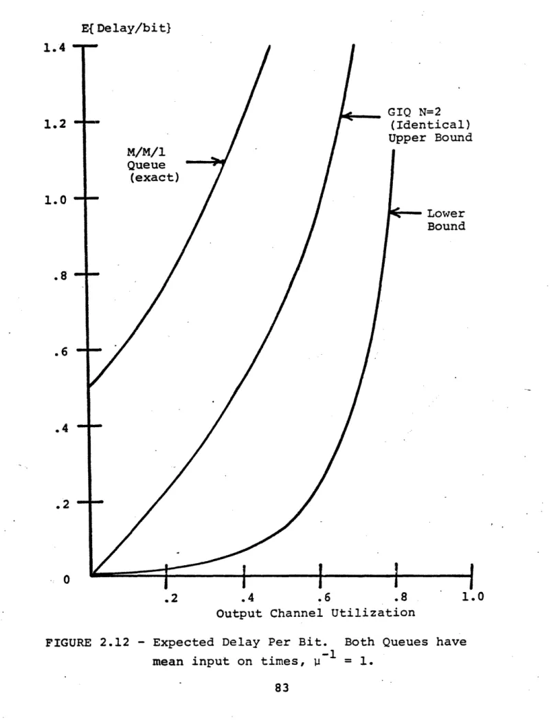
overflow measures are also discussed. A final extension for the single queue is the development of upper and lower bounds for the expected delay per bit through the buffer.

In previous buffering studies of message switched net-works the M/M/1 queue model has been extensively used. The gradual input model is therefore compared to the M/M/1 model. Such a comparison for single queues is presented at the end of Chapter 2. It is shown that the gradual input model enables one to see effects due to a finite number of finite rate traffic sources that are not apparent with the M/M/! model. All of these effects reduce the amount of queueing from that calculated with the /MX/1 model.

The analysis of a network of gradual input queues is presented in Chapter 3. It is first shown that all traffic streams in a general. network are not exactly of the type

required for the analysis presented in Chapter 2. Specifically, all traffic streams will not be alternating renewal processes with exponential off times even if the source traffic streams are of this type. It is shown, however, that if source streams have both exponential on and off times it is a good approxi-mation to assume that all traffic streams in the network are of this type. This is verified mathematically for two

limiting cases and by simulation.

The analysis of a general network of gradual input queues

is then done by first calculating the mean on and off times

associated with all traffic streams. Two sets of linear equations are developed for this purpose. Once the mean traffic parameters have been found, the analysis presented in Chapter 2 can be applied to obtain marginal statistics

for each buffer in the network.

The results for networks of gradual input queues are also compared with those obtained using a network of M/M/l queues. Again the finite source nature of the gradual input model shows network effects that cannot be seen with the M/M/1 model.

Flow control is investigated for tree concentration structures. The flow control is used to eliminate overflows in the interior of the tree. Therefore all overflows occur at source nodes where it would presumably be easy to turn off

the sources. The first problem considered is finding the

buffer allocation in such a tree that minimizes the probability of buffer overflow. It is shown that in certain cases,

placing all buffers at source nodes is the desired allocation. This is not a general result, however. A counterexample is presented that gives insight into why it is not always

desirable to place all buffers at source nodes.

Even though reasonable flow control rules can sometimes be specified, it is often difficult to analyze the performance of the resulting system. To help deal with this problem, an approximate analysis of a small concentration tree using flow control is presented. The analysis is based on a first

passage time theorem for Markov chains. The theorem states that the tail behavior of first passage time distributions is geometric or exponential under fairly general conditions. This is used to develop a stage by stage analysis of a three node system by coupling the dynamics of the nodes in an

approximate way. The results obtained in this way for the system probability of overflow are verified by simulation.

CHAPTER II - THE ANALYSIS OF A SINGLE GRADUAL INPUT QUEUE

Before considering the analysis of an entire message switched network, it is necessary to analyze a single gradual input queue. The first section of this chapter presents the basic definitions and results for the gradual input queueing model due to Rubinovitch, Cohen and Kaspi. In addition,

results for specific cases of interest in this study are obtained and a delay analysis for the queue is developed. The next section considers overflow statistics for a gradual input queue with a finite buffer. The final section compares the gradual input queue with the simpler M/M/1 queue in order to show the insights obtainable from the more detailed model.

2.1 The Basic Gradual Input Queue Model

2.1.1 Definitions and previous results

The following description of the gradual input queue parallels that of Cohen [COHEN 74]. The model represents N incoming channels being multiplexed onto a single outgoing channel as is shown in Figure 2.la. The capacity of each of the incoming channels is the same as that of the outgoing channel, so that when only one incoming channel is on, data passes directly through the multiplexor without buffering or delay. When more than one incoming channel is on, a queue builds up. The buffer is assumed to have infinite capacity and is shared by all incoming channels. The outgoing channel

Inputs

Buffer Output

a. Input and output traffic for each buffer.

on on

off /'/////////,1 of f of

li l, 2,i 2 3,i

b. Input process

FIGURE 2.1 - The gradual input queue

pends data at a constant rate whenever any incoming channel is on or there is data in the buffer.

The on and off process associated with each incoming channel is taken to be an alternating renewal process. As shown in Figure 2.lb, for the ith channel this process is described by the sequence a,i T li a₂,i' 2,i of

statistically independent nonnegative random variables. The random variables a (n = 1,2,3...) represent the successive

n,i

idle periods on the ith channel and the random variables Tni (n = 1,2,3...) represent the lengths of the successive busy periods on that channel. The random variables o have distribution A(') while the random variables Tn have

distri-n,i

bution BC'). The restriction that the processes on all input channels be identically distributed will be removed later.

Figure 2.2 shows the behavior of the gradual input buffer for a specific sample function of the input. A period of continuous inflow into the buffer is called an inflow period and its length is denoted by Qj. The sum of the lengths of all messages flowing into the buffer during the jth inflow period is called the load h.. A busy period of the buffer is a period of uninterrupted flow on the output channel. Its length is denoted by b. The length of time between the start of successive busy periods is called a

busy cycle, whose length is denoted by c. The length of time between the end of the nth and the beginning of the (n+l)st

Buffer Content h-Zk₂ 11 \, o 3_... 30h I _I 61 62 1 63 1 ~-t o-.... 'l ' -, ,._. c"221 e2 2 -- 1 . I _{I I} I Inputs _{- Time}

FIGURE 2.2 - _{The buffering process in a gradual input queue}

(After Fig. 3 in [COHEN 74]) 26

inflow periods is denoted by 6n+l' A final quantity defined by Figure 2.2 is the content of the buffer at the start of the nth inflow period, denoted w.

In order to facilitate the analysis of the gradual

input queue, it is necessary to restrict the distribution of off times on the input channels to be exponential, i.e.

-Xt

A(t) = l-e ; t > 0, X > 0

0 ;t - O

With this restriction, the gaps between inflow periods, 6, are also exponentially distributed (with mean (NA)-). From Figure 2.2 it can be seen that the relationship between

successive buffer contents wn is given by

+

Wn+l [Wn+hn- n-on+_]1 n = 1,2,3...t

Since the 6n are exponentially distributed, the random variables wn correspond to the actual waiting times of an M/G/1 queue with service times hn- n and interarrival times

6n' The actual waiting time in the M/G/l queue is the time

between the arrival of a customer and the start of his service. This equivalence is the basis of the analysis of the gradual input queue.

t [x] = x if x > 0 0 if x - 0

In order to make use of the known results for the M/G/l queue in analyzing the gradual input queue, it is necessary

to obtain the distribution of h n- _n. This has been done by Cohen. The central result is given below. Define

B*(p) = fe -Pt dB(t) Re p - 0 0

8 = rft dB(t)

0

A= N a = A

Theorem (Theorem 2.3 [COHEN 74])

For Re p - 0, Re s > 0, t > 0, Re u > 0 s+A{l-E{exp(-ph-sZ) } 1 =-ut ~e-St 1 e du N f (e (2- i Ce u+X{l-B*(p+u)} co -St fA -2 ut

i e-St exp{ A C u 2e {l-B*(p+u)}du} dt; N=oo

0 2Tri 'C

(Eq.2.1) In this theorem, N=- is the case NA*A as N-+*, X*0. The

integral

ic+Reu

/C eut F(u)du - lim e eut F(u) du

u C-).Os~ -ie+Reu

where s>O andRe u is to the right of all singularities of F(u). Note that 2i eut F(u) du is then the inverse

27ri C Laplace transform of F(u).

Using the above theorem, it is possible to derive the first moments of the distributions of h and X. There are

For

N<-E{2} = (S/a){(l+a/N) - 11 N-l

E{h} = B(l+a/N) (Eq.2.2)

For N=o

E{Q} = (8/a)(ea-l)

E{h} = Bea (Eq.2.3)

For the equivalent M/G/l queue it is known that the queueing process will have a steady state as t-+ only if AE(h-k) < 1. Cohen has shown that for the gradual input queue, the following equivalence exists.

<1 ~ (N-l)X < 1 if N< 1 a < 1 if N=" AE (h-Z) =1 (N-1)XB = 1 if N< a 1 if N=-29

Having found the expected value of h-Z and the conditions under which the queueing process has a steady state, it is now possible to apply the following theorem by Cohen to obtain a useful measure of the buffer build up occurring in a gradual input queue.

Theorem (Theorem 3.4 [COHEN 74])

The maximum content Cmax of the buffer during a busy cycle has the same distribution as the distribution of the maximum virtual waiting time vmax during a busy cycle of an

M/G/1 queue with a service time distribution which is the same as that of h -n and mean interarrival time A 1. The

n n

virtual waiting time, v(t), of the M/G/1 queue is the total remaining service time of the customers in the queue at time t. This is the time a customer would have to wait before

starting service if he arrived at time t. Note that this is not the same as the actual waiting time since v(t) is defined for all t while actual waiting times are defined only at the customer arrival times [COHEN 69].

A result for v of an M/G/1 queue with mean service

max

time x and mean interarrival time d which can now be applied is

-1

E{Vmax} = d log[(l-x/d) (Eq.2.4)

as given in [COHEN 69]. Applying Equations 2.2 and 2.3, one obtains the following.

(

N=-E{Cmax}

-1 -l -l

a {log(l-a (N-l)/N) +(N-l)log(l+a/N)

1}BN<-It is therefore possible to calculate the expected value of the maximum buffer content during a busy cycle in closed form.

Another useful result that has been obtained for the

gradual input queue is the functional form of the distribution

of the busy period on the output channel. Rubinovitch [RUBIN 73] has shown that the output channel of a gradual input

queue has the same busy period distribution as an M/G/1 queue with input rate (N-1)A and service time distribution B(').t If D*(') is the Laplace Stieltjes transform of the distribution of the busy period on the output channel then

D*(e) = B*((N-1)X+

e

e

This is the well known busy period result for an M/G/1 queue [KLEIN 75].

The results so far apply only to a single stage of buffering. It is, however, straight forward to extend the

results to several stages of channels arranged in a converging

tree structure. This is done by observing that the output

tNote that this M/G/1 analogy is not the same as the one used to obtain the previous buffering result.

channel of one stage behaves as an alternating renewal process

as required for it to be the input process to the next stage.

It is therefore possible to analyze a converging tree structure in a stage by stage manner.

This section has been restricted to queues for which all

input channels have identical alternating renewal processes. The results presented here have been generalized to the case of different renewal processest for each input channel by Kaspi and Rubinovitch [KASPI 75]. A summary of their work is given in Appendix A.

2.1.2 Equivalent M/G/1 queue service time analysis

In the previous section it was shown that the queueing process in a gradual input queue can be analyzed by making an analogy with an M/G/1 queue. The equivalent M/G/l service time distribution is the same as the distribution of h-Z, the queue buildup during an inflow period of the gradual input queue. In this section the Laplace transform of the distri-bution of h-R is obtained for specific cases. The specific cases considered are ones in which the on times, T_i j, as well as the off times, ai ; -on the input channels are

exponentially distributed. These special cases are required for the analysis of the general networks presented in

Chapter 3.

tThe off periods on each channel are still required to be exponentially distributed.

The results presented here are obtained by using a

Markov chain representation for the behavior of the input channels to the queue. This approach is easier to understand

than using the relationship given by Cohen for E{exp(-ph-s)}.T

It also allows one to analyze queues for which the input channel capacity is larger than that of the output channel.

Cohen's result (Theorem 2.3 [COHEN 741) is stated in the previous section. Note that it gives E{exp(-ph-sZ)} for

Re P - 0, Re s > 0. Therefore in order to use the result

to obtain E{exp(-p(h-Z))} analytic continuation must be used. Appendix A-4 of [COHEN 74] shows how to do this for the case of an infinite number of input>channels (N=c). The result for this case is that for p - 0,

p-A{l-B (p) }

p-AT1-Etexp -p (h-.T)] }

=- -Af E{exp [-p (B-t) (Bpt) }exp[ A u 2e ut{1-(p+u)

0 u

du]dt

1 if B-t

Where B has distribution B(') and (B-t) = 0 otherwise

The alternating on/off renewal process associated with a communication channel on which these times are exponentially distributed can be represented as a two state continuous

time Markov chain. Let the off times have distribution function

A(t) = 1-e t - t > O, X > O

o

t

0o

and the on times have distribution function

B(t) = 1-e- u t t > 0, j > 0

O t O 0

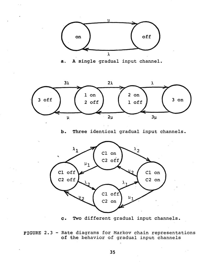
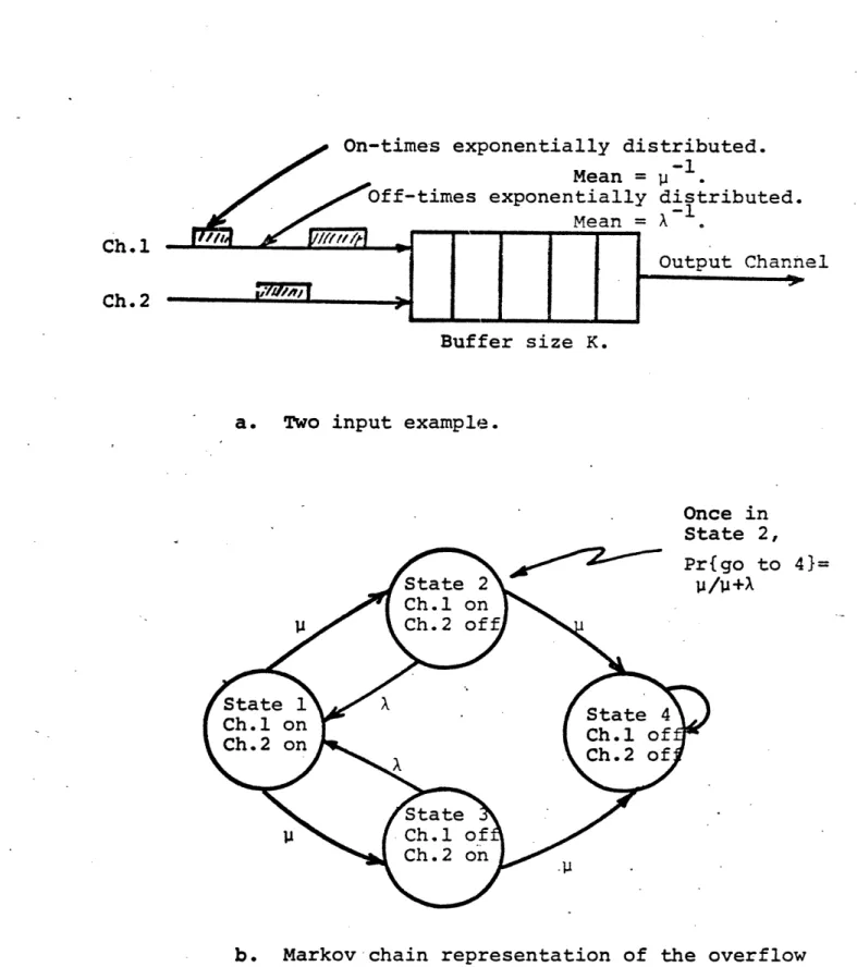
Then the behavior of the channel can be represented by the Markov chain shown in Figure 2.3a. If there are N independent

input channels, their joint behavior can also be represented by a Markov chain. The chain representing the joint behavior of three identical input channels is shown in Figure 2.3b.

The states of the chain are the number of channels on and the number off. The transition times between the states are

exponentially distributed as required for the system to be a continuous time Markov chain. This follows from the memory-less property of the exponential distribution and the fact

a. A single gradual input channel.

3X 2X A

1 on 2 on

2 off 1 off3

11 ' 21 13

b. Three identical gradual input channels.

X1 n, C2 off C1 of C1 on C2 off C2 on C1 o ,~ C2 on

c. Two different gradual input channels.

FIGURE 2.3 - Rate diagrams for Markov chain representations of the behavior of gradual input channels

that the time to a state transition is given by the minimum of a set of independent exponential distributions (the set of times until the next transition on each channel). It is well known that the minimum of such a set is exponentially

distributed.

It is also straightforward to extend the Markov chain representation to independent input channels with different

traffic parameters. Figure 2.3c illustrates the Markov

chain for the joint behavior of two input channels with mean on and off times (p1 A ) and (p 2 21)

Now recall that the quantity h-Z is the queue buildup during an inflow period of the gradual input queue. This

time period can easily be identified in the Markov chain representation of the input channels. An inflow period starts with a transition from all inputs off to one input on and ends on the first return to the state with all inputs

off. Therefore an inflow period is a first passage event in this Markov chain.

The excess queue buildup, h-Z, during this first passage event can now be identified. This can be done for queues with input channel capacities, Ci, which are greater than or

equal to the output channel capacity, CO. For such a queue,

whenever the input channels are in a state with N input on

channels on, the buffer content of the queue increases at rate rb, where

rb Non Ci - Co Non 1 C C (Eq.2.5)

Equation 2.5 can now be used to scale the transition time distributions for the input channel Markov chain so that the time spent in each state represents the excess queue buildup while in that state. In the resulting scaled Markov chain, the time for the first passage event that starts from the all channels off state with one input coming on and ends upon the first return to the all off state is equal to the quantity h-1.

The use of the scaled Markov chain to determine the Laplace transform H*(s) of the distribution of h-Z is best illustrated by an example. The unscaled Markov chain

representing three identical gradual input channels was shown in Figure 2.3b. If these channels have capacity C_i = C_o = 1, then the scaled Markov chain representing the rate of queue buildup will be as shown in Figure 2.4. Note that state 1 (all channels off) is shown as a trapping state because it is the end state of the first passage event of interest. As such, the time until trapping in state 1 will be the same as the first passage time to that state. Also note that since there is no queue buildup in state 2 (one input on), there are infinite transition rates out of this state in the scaled chain.

m,-I 4.1 I ! 1. I:: 4.J IC)d4.Jrl J~~~~~4 I~~ ~ ~ ~~~~~~I -~,_{0 t4} cl: _{Z QZ ·w A}Ca*~1 0'1 W Or < ll -~~~~t a "~ II u J aa ~,,-ac sm a \ itCro~ l a>rl 1 a, Jt ·rl ·_0 O _Z I 3 ·cr _{/ .cC} I _I I>_k ,1 tw OO :2: Z Z ~qla rl. 4J 00 fq ri t d G O i 44'

38Z

Let x(t) be the state of the scaled Markov chain. Then, as discussed previously, h-i is equal to the following first passage time

h-t = f21 = inf{t; x(t)=lJx(0) = 21

If f₂₁(t) is the probability density function of f2 1 then

the desired transform is

F*(s)= H*(s) = e f-s t₂ )dt

21 2(t)dt

t=o

This transform can be found by general methods, such as those given by. Howard [HOWD 71], or by taking advantage of the

special structure of the chain as discussed below. In either case, transition probabilities pij=Pr {next state=jjcurrent state=il and waiting time probability density functions wi (t) must be identified. For the chain shown in Figure 2.4, the matrix of transition probabilities is

1 o 0 O 2X

o

O

The density functions wij(t) are the densities of the time until transition, given that a transition from state i to j will occur, and zero if a direct transition is not possible

from i to j. For the continuous time Markov chain under

consideration here, these are all exponential. The mean times are the mean time spent in each state. Therefore the matrix of these densities is wll(t) 0 O O 6(t) 0 6(t) 0 0 +2X) e (,w+2X)e- (+ 2 X)t 3U -_ 3 0 0 20it 0 2 u z

Where 6(t) is the Dirac delta 6(t) = {1 t=0

0 otherwise

Since state 1 is a trapping state, wl!(t) can be any probability density function such that wll(t) = 0 if t < 0.

From the matrix W(t) it is easy to generate the matrix of Laplace transforms of the waiting time densities.

w*l (s)0 0 0

1 0 1 0

W* (s =

Because of the simple structure of the Markov chain, the transform Fi (s) can easily be found by the following method. Let Y₂₃ and y_{3 4} be the number of state 2 to state 3 and

state 3 to state 4 transitions that are made during the first passage event starting from state 2 and ending in state 1. Knowing Y2 3 and y3 4 is equivalent to knowing the

number of times states 2, 3, and 4 were entered before the trapping state 1 was reached. The transform Fl1(s) can

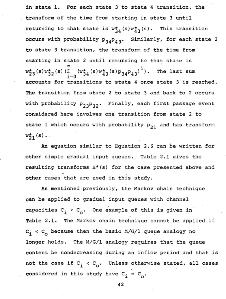
therefore be found by summing conditional transforms as follows 21( = {Fl(S) IY23=J Y34 k} 1(S) = ~All possible j,k Pr{Y_{2 3}=j, Y₃₄=k} -w21 (S)P21 (23 (s)32(s)) All possible j,k (w34(s)w43(s)) (P23P32) (P34P43 - zo = W ₁(s)p₂ E (w ₃(s)w* (s) ₂ (E (w* (s)W_{4 3} (S) 21 21 j=0 23 3 i= 34 43 . . P₃4P_{3 2}) )P_{2 3}P 32)3 (Eq.2.6)

Equation 2.6 states that there can be j=0,1,2... transitions from state 2 to state 3 and for each of these there can be

i=0,1,2,... transitions from state 3 to state 4 before trapping

in state 1. For each state 3 to state 4 transition, the transform of the time from starting in state 3 until

returning to that state is w 4 (s)w 3 (s). This transition

occurs with probability P_{3 4}P _{4 3}. Similarly, for each state 2 to state 3 transition, the transform of the time from

starting in state 2 until returning to that state is w* (s)w₃ * (s)( ₂ (w* (s)w_{4 3} (s)P_{3 4}P₄₃)i). The last sum

i=O

accounts for transitions to state 4 once state 3 is reached. The transition from state 2 to state 3 and back to 2 occurs with probability P_{2 3}P_{3 2}. Finally, each first passage event considered here involves one transition from state 2 to

state 1 which occurs with probability P_{2 1} and has transform

w" (s).

21

An equation similar to Equation 2.6 can be written for other simple gradual input queues. Table 2.1 gives the resulting transforms H*(s) for the case presented above and other cases that are used in this study.

As mentioned previously, the Markov chain technique can be applied to gradual input queues with channel

capacities Ci > Co. One example of this is given in

Table 2.1. The Markov chain technique cannot be applied if C_i < C_o because then the basic M/G/1 queue analogy no

longer holds. The M/G/l analogy requires that the queue content be nondecreasing during an inflow period and that is not the case if C_i < C_o. Unless otherwise stated, all cases considered in this study have Ci = CO.

eq 0C) oxc o4 U n .,< O O 4J + + + . U Q I I ·el < + .e W * n UZ e C) N a _- %D IR + + *,1 ,t + . o + rt i, i , CN _ II N V II (a '. -< > O + N ,+ --4i C) - ). + < ._l . _ n+ ++ a r.-4 m' + oq . N + .-- I > I -- ~ = -- _ -44) c< . .C : N + ; 9: .r4 _+ a eq < 3 =(1) C) U 1n n + N + + m : 1c I N- eq + N _ q O 04 04 Q , < 4 < CN 4 304 EI d X , - N iX *: --I U ;::I. ._< ~ ; + : H -04(0 a ) - N + + ko u) a e .. C - eN +D - + + .r 4 ( 44 R + C< Ucn (e CN CeU 0 0) 'W II -_i N ₊ r O n - < ko oN + H H ia -r q d CN + r sR H < * S 4c s .C + + u) n + eq V C U - 2 + 2 = + e CN e C44 -w * _ .N N- + e q + f Oro .c 9f: 4- I co + 4J (a r4 0 + r i E I + H ,- - _ I..- i e4 f. L,1:(a WUO Srd c + _ + 1i :5tl")3 e N _ - . + C-tr I- co :I eq 0 rn E 04- (3) O + r_ - C U N CN 44 O E m + Hl+ ' Cd 3 _ 0W .-.ir 0 z W H I 0 1. C43 (n a XC U r1 C) _ ,_ _ U,1 Crd U} _C) 04 _{C) 4} H r *o04 - *d (U 'U 43

There is another approach to finding F* (s) that can be

used. Howard [HOWD 71] gives the result that the matrix of

first passage time distributions for a continuous time Markov chain satisfies the following relationship.

F*(s) = C*(s) [(I-C*(s)) l][(I-(s))- 1D I]

-(Eq.2.7)

The matrix C*(s) is ,alled the core matrix. It is defined as follows

*(s) = P (W* s)

The operatorD in the above equations signifies element by element multiplication of the two matrices. For the gradual input queues considered in this study it is easier to write an equation like Equation 2.6 than to perform the matrix inversions required in Equation 2.7. The infinite sums in Equation 2.6 are all simple geometric sums for which closed form expressions exist.

2.1.3 Bounds for the expected delay per bit

A performance measure that is often of interest for

message switched communication networks is delay. In

previous studies using the M/M/1 queue as a model, the delay measure usually considered was expected delay per message. For the gradual input model this measure is difficult to find because tihe distributions obtained for buffer content are not expressed in terms of number of messages. Instead buffer contents are expressed in terms of time units of work

(for the output channel) which represent bits when normalized by the communication rate of the output channel. Therefore an expected delay per bit measure will be used for the

gradual input queue.

The delay experienced by a specific bit in a gradual input queue is a function of the queue contents at the time of its arrival and of the service discipline of the queue. The service discipline in the queue may be difficult to

represent mathematically. For example, suppose that messages are sent on a first-come-first-served (FCFS) basis. Then the bits are not sent strictly FCFS. Fortunately, as long as the service discipline is work conserving, the mean delay per bit remains unchanged. Therefore the mean delay per bit can be found assuming FCFS service for all bits.

tThis follows from Little's formula [LTTL 61], L=XW, which says that the expected delay W for a aueue equals the expected queue size L divided by the mean arrival rate X. All work conserving service disciplines give the same expected queue

size in terms of bits for the gradual input queue.

With the FCFS service discipline, it is easy to see that

the delay for a specific bit db is

db = buffer content at time of bit arrival

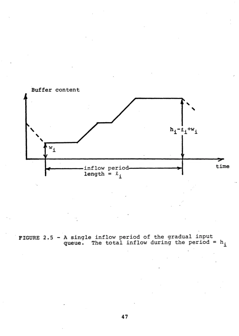
For the gradual input queue, this means that only the queue size during inflow periods is of interest since that is the only time during which bits arrive. Figure 2.5 shows the buffer

content

the exact delay per bit during this period is very difficult. However, this delay can easily be bounded. Note that at the start of the inflow period the delay (buffer content) is w. while at -the end it is hi-Zi+wi. The delay is strictly

nondecreasing during the inflow period. If one considers M inflow periods, the average delay per bit is bounded by

M M Z h.iwi hi [hi-i+wi ] i=l 1 2 < - < i=l M db M

Z

Taking the limit as M-o and making an ergodic argument gives

E[hw] < < E [h(h-2+w) ]

E[h] -E[db] - E[h]

Buffer content

1 W

hi- i+Wi

W.

inflow period . time

length = Zi

FIGURE 2.5 - A single inflow period of the gradual input queue. The total inflow during the period = h

Since h_i and w _i are independent, these bounds simplify to

E[w] E[d_{b ]} E(h] _E[h] + E[w] (Eq.2.8)

Now recall that w is the actual waiting time of an

equivalent M/G/1 queue. Assume that the gradual input queue has N input channels with mean off times i- 1 (i = 1,2,..N)

Then the equivalent M/G/1 queue has mean interarrival time

N -1

( lAi)-i and a service time distribution equal to the

dis-i=l

tribution of h-Z. Therefore E[w] can be found using the well known Pollaczek-Khintchine formula [KLEIN 75] for the mean waiting time in an M/G/1 queue.

XT E[(h-2)2 ]

E[w] 2(1-A E[(h-Q-)I) (Eq.2.9)

N

where XT Z i.

Equation 2.9, together with Equation 2.8, gives both upper and lower bounds on E[db] in terms of first and second moments of the fundamental quantities h and Z. An example

of the bounds is given in Section 2.3.

2.2 The Gradual InPut Queue With A Finite Buffer

2.2.1 Probability of buffer overflow in a busy period

A probability of buffer overflow measure is required

in order to be able to use the gradual input queueing model to study buffering requirements for a communication network. The key to calculating a probability of buffer overflow for this queueing model with a finite buffer is to use a

pro-bability that is convenient to work with. The most convenient is the probability of one or more buffer overflow events

during a busy period, and this is the measure used in this study. This measure is convenient because the start of each busy period is a renewal point for the queueing process in the gradual input model. At this point, all but one of the inputs are off with an exponentially distributed time

remaining until they come on again. In addition, the buffer is empty so that, stochastically, a queue with an infinite buffer and one with a finite buffer behave identically from the start of a busy period until the finite buffer overflows. For any busy period then, the probability of no overflow for

the finite buffer is the same as the probability that the buffer content of the infinite buffer never crosses the

level equal to the size of the finite buffer during the busy period.

The analogy between the contents of a gradual input queue and the virtual waiting time in an M/G/1 queue can now

be applied. For a gradual input queue with buffer size K

No overflow during) v K during a busy period)

Pr(_a busy period Pr( ax

of equivalent M/G/1 queue

where the equivalent M/G/1 queue has an infinite buffer, a

mean interarrival time of A-1 and a service time distribution that is the same as the distribution of h-Z. Let w be the actual waiting time for the equivalent M/G/1 queue and y be a random variable with the same distribution as the service time. Then the following result for an M/G/1 queue can be

used

Pr(v = Pr(w+y-K) -K) (Eq.2.10)

Ref. [COHEN 69] p. 525 [TAKACS 65] p. 381

By using the fact that Pr(v >K)=l-Pr(v -K), Equation 2.10

max max

provides a way of theoretically calculating the probability of one or more overflow events during the busy period of the gradual input queue with buffer size K. Specifically,

POverflow during) =1 <K)<Pr(v

rbusy period max

Pr(w-K) - Pr(w+v-K)

Pr (wlK)

Pr(w+y>K) - Pr(w>K)

1-Pr(w>K)

Because the distributions of w and y for the M/G/1 .queue analogy are fairly complicated, it is worthwhile

trying to bound the probability of overflow rather than calculating it exactly. This can be done by applying the exponential bounds on the waiting time in G/G/1 queues developed by Kingman [KING 70]. For a G/G/1 queue, denote the service time of the nth customer by xn and the interval between arrivals of the (n+l)st and nth customer by tn. Now

define the random variable yn by

Yn = Xn - tn

The yn'& are i.i.d. random variables, therefore they have a common distribution function F(u) = Pr{y<u}. Kingman has shown that

-e'*K < < Pwe* K

r e Pr{w>K-e (Eq.2.12)

where the constant r is given by

r = inf t>₀ dF(u)/lfe (u-t) dF(u)

t t

and e* is the unique greatest positive real root of the equation

f(e) = f eeu dF(u) = 1 (Eq.2.13)

in an interval I in which f(8) is bounded. This interval I includes the origin 0=0 since f(0)=l. Furthermore, it can be shown that f(0) is a convex U functiont and that f'(O) =

E{x-t}<O for a queue with a utilization <1. It can also be seen that

f(e) = A*(e)B*(-e) (Eq.2.14)

where A*(e) and B*(O) are the Laplace transforms of the

interarrival time, t, _n and service time, xn, distributions

respectively.

The bound in Equation 2.12 can be applied to Equation 2.11 yielding

Pr(overflow) < Pr (Eq.2.15)

1

The problem now is to bound the Pr(w+y>K). This can be done by noting that

K

Pr(w+y>K) = Pr(y>K) + f Pr(w>(K-t)) dH(t) t=O

where H(t) is the distribution function of h-Z.

tThe function f(8) is convex U if

Using the fact that Pr(y>K) = f dH(t) and that t=K

Pr(w>O) = 1, one obtains

Pr(w+y>K) = f Pr (w> (K-t))dH(t) e (Kt) dH(t)

t=o t=o

-OK

= H*(-8)e (Eq.2.16)

This expression for ?r(w+y>K) can be substituted into

Equation 2.15 giving the following exponential bound on the probability of one or more overflows during a busy period of a gradual input queue with buffer size K.

-OK

Pr (overflow) (H*- (Eq.2.17)

1 -e

This exponential bound can be applied in a straightforward

manner except for the constant r. The constant r is difficult to determine exactly in general. Fortunately, however, it is easy to see from its definition that r-O. Therefore setting

r=O still gives an upper bound, i.e.

-OK

Pr(overflow) < H*(-8)e (Eq.2.18)

1 - e

The effect of letting r=O is to weaken the bound, but the correct exponential behavior is preserved. The next section gives an example that illustrates this effect.

It is desirable to have a lower bound as well as an .upper bound on the Pr(overflow) as defined in this section.

One can start with Equation 2.10 and apply the Kingman

bounds on waiting time to obtain a lower bound, but in this case, since the constant r cannot be determined, the bound is useless. Therefore the alternative that will be used is to realize that for a gradual input queue

Pr(overflow) = E Pr(Overflow in ith inflow period) i=l

Pr(Overflow in lst inflow period)

= Pr(h-2>buffer size) (Eq.2.19)

Here only the first inflow period has been used to obtain a lower bound. If a tighter bound is desired, more inflow periods can be considered.

The bounds developed here for Pr(overflow) are

illustrated with examples in the next section that indicate their tightness.

2.2.2 Examples of the bounds on Pr(Overflow)

Two examples of the use of the bounds on Pr(overflow) are given in this section. The first is a gradual input queue which is used to illustrate the general procedure.

The second is an M/M/1 queue which is presented to show how the upper bound compares with the exact value.

As a first example, consider a gradual input queue with three identical input channels. The on and off times on each channel are exponentially distributed with means - =1 and X =5 respectively. This gives an output channel utilization of 0.5 if no traffic losses occur.

As described previously, the Pr(overflow) for this queue with buffer size K can be determined by considering an equivalent M/G/1 queue. The equivalent M/G/1 queue has an interarrival time distribution with Laplace transform

3X 0.6 A+3A +0.6

This is the transform for the time between inflow periods.

The transform for the equivalent service time is the same as the transform of h-k.

B*(8) = H*(e) = 2uO2+(2Xu+7U2)0+6'3

(2u+4X)0 +(4X +2Xp+72 )e+63i

282 + 7.40 + 6

2

2.80 + 8.768 + 6

Now the problem is to find the exponent 8* for the exponential bound. The exponent is the unique positive

real solution to

f(e) = A*(e)B*(-8) = 1

which lies in an interval I. in which f(8) is bounded. For

the example considered here, this equation has three solutions, 0, 0.902 and 2.055. Of these, only 0.902 is positive real

and in I8. The root 2.055 lies outside of TI because the

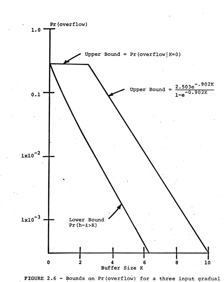
function B*(-e) has a pole at 1.01. The uniqueness of 8* is therefore as predicted by the Kingman theory. The bound is completed by finding H*(-e*) = H*(-0.902) = 2.503 Therefore -0.902K < 2.503e Pr(overflow) 2 -0.902K i-e

where K is the buffer size. This bound is plotted in Figure 2.6. Notice that for small values of K the bound becomes large because of the denominator. Therefore another bound has been used in this region.

The bound used for small buffer sizes is the Pr(overflow) when K=0. For K=0 the following is true.

l-Pr(overflow) = Pr(First input channel goes off before a second one comes on)

Pr (overflow) 1.0

Upper Bound = Pr(overflow|K=O)

2.503e Upper Bound = 1_-' 9 2_0K 0.1 1-e 0.902K 1x10- 2 1x10 Lower Bound Pr(h-Q>K) 0 2 4 6 8 10 Buffer Size K

FIGURE 2.6 - Bounds on Pr(overflow) for a three input gradual input queue. All three inputs are identical with

-1 -1

j =1 and X =5. 57

ontime t off time>t 2 i Prfor channel (Pr for channel )) dt

_ f -Ut -At -At

=-oje e e dt

t=0

_

u 1

- +2X = .4 = 0.714

Clearly this exact solution for K=0 is an upper bound for K>0. The lower bound to Pr(overflow) that was developed in the previous section is

Pr(overflow) - Pr(h-Z>K)

In order to evaluate this bound, the transfornm H*(8) must be inverted. For this example

28 + 7.48 + 6 H*"() = 2

2.80 + 8.768 + 6

0.4080 + 0.612 (8+1.013) (6+2.116)

Therefore using standard inversion techniques, one obtains

H(t)=0.7146(t)+(.178) (1.013)e '013t+(.108)(2.116)e t t-0 where ₆(t) = 1 if t=O

= 0 otherwise