HAL Id: hal-00569095
https://hal.archives-ouvertes.fr/hal-00569095v2
Submitted on 10 Jun 2011
HAL is a multi-disciplinary open access
archive for the deposit and dissemination of
sci-entific research documents, whether they are
pub-lished or not. The documents may come from
teaching and research institutions in France or
L’archive ouverte pluridisciplinaire HAL, est
destinée au dépôt et à la diffusion de documents
scientifiques de niveau recherche, publiés ou non,
émanant des établissements d’enseignement et de
recherche français ou étrangers, des laboratoires
An Elementary affine λ-calculus with multithreading and
side effects (extended version)
Antoine Madet, Roberto M. Amadio
To cite this version:
Antoine Madet, Roberto M. Amadio. An Elementary affine λ-calculus with multithreading and side
effects (extended version). 2011. �hal-00569095v2�
An Elementary Affine λ-calculus
with Multithreading and Side Effects
∗
Antoine Madet
Roberto M. Amadio
Laboratoire PPS, Universit´
e Paris Diderot
{madet,amadio}@pps.jussieu.fr
Abstract
Linear logic provides a framework to control the complexity of higher-order functional programs. We present an extension of this framework to programs with multithreading and side effects focusing on the case of elementary time. Our main contributions are as follows. First, we provide a new combinatorial proof of termination in elementary time for the func-tional case. Second, we develop an extension of the approach to a call-by-value λ-calculus with multithreading and side effects. Third, we introduce an elementary affine type system that guarantees the standard subject re-duction and progress properties. Finally, we illustrate the programming of iterative functions with side effects in the presented formalism.
∗Work partially supported by project ANR-08-BLANC-0211-01 “COMPLICE” and the
Future and Emerging Technologies (FET) programme within the Seventh Framework Pro-gramme for Research of the European Commission, under FET-Open grant number: 243881 (project CerCo).
Contents
1 Introduction 3
2 Elementary Time in a Modal λ-calculus 4
2.1 A Modal λ-calculus . . . 4
2.1.1 Syntax . . . 4
2.1.2 Operational Semantics . . . 5
2.2 Depth System . . . 5
2.3 Elementary Bound . . . 7
3 Elementary Time in a Modal λ-calculus with Side Effects 10 3.1 A Modal λ-calculus with Multithreading and Regions . . . 10
3.1.1 Syntax . . . 10
3.1.2 Operational Semantics . . . 11
3.2 Extended Depth System . . . 12
3.3 Elementary Bound . . . 14
4 An Elementary Affine Type System 16 5 Expressivity 19 5.1 Completeness . . . 19
5.2 Iteration with Side Effects . . . 19
6 Conclusion 21 A Proofs 23 A.1 Proof of theorem 3.5 . . . 23
A.2 Proof of proposition 3.6 . . . 27
A.3 Proof of lemma 2.8 . . . 28
A.4 Proof of theorem 3.7 . . . 29
A.5 Proof of proposition 4.1 . . . 31
A.6 Proof of theorem 4.4 . . . 32
A.6.1 Substitution . . . 32
A.6.2 Subject Reduction . . . 33
A.6.3 Progress . . . 34
A.7 Proof of theorem 5.3 . . . 36
A.7.1 Successor, addition and multiplication . . . 37
A.7.2 Iteration schemes . . . 38
A.7.3 Coercion . . . 39
A.7.4 Predecessor and subtraction . . . 39
A.7.5 Composition . . . 40
1
Introduction
There is a well explored framework based on Linear Logic to control the com-plexity of higher-order functional programs. In particular, light logics [11, 10, 3] have led to a polynomial light affine λ-calculus [13] and to various type sys-tems for the standard λ-calculus guaranteeing that a well-typed term has a bounded complexity [9, 8, 5]. Recently, this framework has been extended to a higher-order process calculus [12] and a functional language with recursive def-initions [4]. In another direction, the notion of stratified region [7, 1] has been used to prove the termination of higher-order multithreaded programs with side effects.
Our general goal is to extend the framework of light logics to a higher-order functional language with multithreading and side effects by focusing on the case of elementary time [10]. The key point is that termination does not rely anymore on stratification but on the notion of depth which is standard in light logics. Indeed, light logics suggest that complexity can be tamed through a fine analysis of the way the depth of the occurrences of a λ-term can vary during reduction.
Our core functional calculus is a λ-calculus extended with a constructor ‘!’ (the modal operator of linear logic) marking duplicable terms and a related let ! destructor. The depth of an occurrence in a λ-term is the number of !′s that
must be crossed to reach the occurrence. Our contribution can be described as follows.
1. In Section 2 we propose a formal system called depth system that con-trols the depth of the occurrences and which is a variant of a system proposed in [13]. We show that terms well-formed in the depth system are guaranteed to terminate in elementary time under an arbitrary reduction strategy. The proof is based on an original combinatorial analysis of the depth system ([10] assumes a specific reduction strategy while [13] relies on a standardization theorem).
2. In Section 3, following previous work on an affine-intuitionistic system [2], we extend the functional core with parallel composition and operations producing side effects on an ‘abstract’ notion of state. We analyse the im-pact of side-effects operations on the depth of the occurrences and deduce an extended depth system. We show that it still guarantees termination of programs in elementary time under a natural call-by-value evaluation strategy.
3. In Section 4, we refine the depth system with a second order (polymorphic) elementary affine type system and show that the resulting system enjoys subject reduction and progress (besides termination in elementary time). 4. Finally, in Section 5, we discuss the expressivity of the resulting type system. On the one hand we check that the usual encoding of elementary functions goes through. On the other hand, and more interestingly, we provide examples of iterative (multithreaded) programs with side effects.
The λ-calculi introduced are summarized in Table 1.1. For each concur-rent language there is a corresponding functional fragment and each language (functional or concurrent) refines the one on its left hand side. The elementary complexity bounds are obtained for the λ!
δ and λ!Rδ calculi while the progress
property and the expressivity results refer to their typed refinements λ! EA and
λ!R
EA, respectively. Proofs are available in Appendix A.
Functional λ! ⊃ λ!
δ ⊃ λ!EA
∩
Concurrent λ!R ⊃ λ!R
δ ⊃ λ!REA
Table 1.1: Overview of the λ-calculi considered
2
Elementary Time in a Modal λ-calculus
In this section, we present our core functional calculus, a related depth system, and show that every term which is well-formed in the depth system terminates in elementary time under an arbitrary reduction strategy.
2.1
A Modal λ-calculus
We introduce a modal λ-calculus called λ!. It is very close to the light affine
λ-calculus of Terui [13] where the paragraph modality ‘§’ used for polynomial time is dropped and where the ‘!’ modality is relaxed as in elementary linear logic [10].
2.1.1 Syntax
Terms are described by the grammar in Table 2.1: We find the usual set of M, N ::= x, y, z . . . | λx.M | M N | !M | let !x = N in M
Table 2.1: Syntax of λ!
variables, λ-abstraction and application, plus a modal operator ‘!’ (read bang) and a let ! operator. We define !0M = M and !n+1M = !(!nM ). In the terms
λx.M and let !x = N in M the occurrences of x in M are bound. The set of free variables of M is denoted by FV(M ). The number of free occurrences of x in M is denoted by FO(x, M ). M [N/x] denotes the term M in which each free occurrence of x has been substituted by the term N .
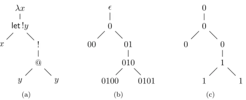
Each term has an abstract syntax tree as exemplified in Figure 2.1(a). A path starting from the root to a node of the tree denotes an occurrence of the program that is denoted by a word w ∈ {0, 1}∗(see Figure 2.1(b)).
λx let!y x ! @ y y (a) ǫ 0 00 01 010 0100 0101 (b) 0 0 0 0 1 1 1 (c)
Figure 2.1: Syntax tree of the term λx.let !y = x in !(yy), addresses and depths
Definition 2.1(depth). The depth d(w) of an occurrence w is the number of !’s that the path leading to w crosses. The depth d(M ) of a term M is the maximum depth of its occurrences.
In Figure 2.1(c), each occurrence is labelled with its depth. Thus d(λx.let !y = x in !(yy)) = 1. In particular, the occurrence 01 is at depth 0; what matters in computing the depth of an occurrence is the number of ! that precedes strictly the occurrence.
2.1.2 Operational Semantics
We consider an arbitrary reduction strategy. Hence, an evaluation context E can be any term with exactly one occurrence of a special variable [ ], the ‘hole’. E[M ] denotes E where the hole has been substituted by M . The reduction rules are given in Table 2.2. The let ! is ‘filtering’ modal terms and ‘destructs’ the
E[(λx.M )N ] → E[M [N/x]] E[let !x = !N in M ] → E[M [N/x]] Table 2.2: Operational semantics of λ!
bang of the term !N after substitution. In the sequel, → denotes the reflexive∗ and transitive closure of →.
2.2
Depth System
By considering that deeper occurrences have less weight than shallow ones, the proof of termination in elementary time [10] relies on the observation that when reducing a redex at depth i the following holds:
(1) the depth of the term does not increase,
(3) the number of occurrences at depth i strictly decreases,
(4) the number of occurrences at depth j > i may be increased by a multi-plicative factor k bounded by the number of occurrences at depth i + 1. Theses properties can be guaranteed by the following requirements: (i) in λx.M , x may occur at most once in M and at depth 0,
(ii) in let !x = M in N , x may occur arbitrarily many times in N and at depth 1.
Hence, the rest of this section is devoted to the introduction of a set of inferences rules called depth system. Every term which is valid in the depth system will terminate in elementary time. First, we introduce the judgement:
Γ ⊢δ M
where δ is a natural number and the context Γ is of the form x1: δ1, . . . , xn: δn.
We write dom(Γ) for the set {x1, . . . , xn}. It should be interpreted as follows:
The free variables of !δM may only occur at the depth specified
by the context Γ.
The inference rules of the depth system are presented in Table 2.3. Γ, x : δ ⊢δx Γ, x : δ ⊢δ M FO(x, M ) ≤ 1 Γ ⊢δ λx.M Γ ⊢δM Γ ⊢δN Γ ⊢δM N Γ ⊢δ N Γ, x : (δ + 1) ⊢δ M Γ ⊢δ let!x = N in M Γ ⊢δ+1M Γ ⊢δ!M
Table 2.3: Depth system: λ! δ
We comment on the rules. The variable rule says that the current depth of a free variable is specified by the context. The λ-abstraction rule requires that the occurrence of x in M is at the same depth as the formal parameter; moreover it occurs at most once so that no duplication is possible at the current depth (Property (3)). The application rule says that we may only apply two terms if they are at the same depth. The let ! rule requires that the bound occurrences of x are one level deeper than the current depth; note that there is no restriction on the number of occurrences of x since duplication would happen one level deeper than the current depth. Finally, the bang rule is better explained in a bottom-up way: crossing a modal occurrence increases the current depth by one.
Definition 2.2 (well-formedness). A term M is well-formed if for some Γ and δ a judgement Γ ⊢δ M can be derived.
Example 2.3. The term of Figure 1(a) is well-formed according to our depth system: x : δ ⊢δx x : δ, y : δ + 1 ⊢δ+1y x : δ, y : δ + 1 ⊢δ+1y x : δ, y : δ + 1 ⊢δ+1yy x : δ, y : δ + 1 ⊢δ!(yy) x : δ ⊢δ let!y = x in !(yy) ⊢δ λx.let !y = x in !(yy)
On the other hand, the followings term is not valid: P = λx.let !y = x in !(y!(yz))
Indeed, the second occurrence of y in !(y!(yz)) is too deep of one level, hence reduction may increase the depth by one. For example, P !!N of depth 2 reduces to !(!N !(!N )z) of depth 3.
Proposition 2.4(properties on the depth system). The depth system satisfies the following properties:
1. If Γ ⊢δ M and x occurs free in M then x : δ′ belongs to Γ and all
occur-rences of x in !δM are at depth δ′.
2. If Γ ⊢δ M then Γ, Γ′⊢δM .
3. If Γ, x : δ′ ⊢δ M and Γ ⊢δ′
N then d(!δM [N/x]) ≤ max (d(!δM ), d(!δ′
N )) andΓ ⊢δM [N/x].
4. If Γ ⊢0M and M → N then Γ ⊢0N and d(M ) ≥ d(N ).
2.3
Elementary Bound
In this section, we prove that well-formed terms terminate in elementary time under an arbitrary reduction strategy. To this end, we define a measure on terms based on the number of occurrences at each depth.
Definition 2.5 (measure). Given a term M and 0 ≤ i ≤ d(M ), let ωi(M ) be
the number of occurrences in M of depth i increased by 2 (so ωi(M ) ≥ 2). We
define µi
n(M ) for n ≥ i ≥ 0 as follows:
µi
n(M ) = (ωn(M ), . . . , ωi+1(M ), ωi(M ))
We write µn(M ) for µ0n(M ). We order the vectors of n + 1 natural number with
the (well-founded) lexicographic order > from right to left.
We derive a termination property by observing that the measure strictly decreases during reduction.
Proposition 2.6(termination). If M is well-formed, M → M′ andn ≥ d(M )
thenµn(M ) > µn(M′).
Proof. We do this by case analysis on the reduction rules: • M = E[(λx.M1)M2] → M′= E[M1[M2/x]]
Let the occurrence of the redex (λx.M1)M2be at depth i. The restrictions
on the formation of terms require that x occurs at most once in M1 at
depth 0. Then ωi(M ) − 3 ≥ ωi(M′) because we remove the nodes for
application and λ-abstraction and either M2 disappears or the occurrence
of the variable x in M1 disappears (both being at the same depth as the
redex). Clearly ωj(M ) = ωj(M′) if j 6= i, hence
µn(M′) ≤ (ωn(M ), . . . , ωi+1(M ), ωi(M ) − 3, µi−1(M )) (2.1)
and µn(M ) > µn(M′).
• M = E[let !x =!M2 inM1] → M′= E[M1[M2/x]]
Let the occurrence of the redex let !x =!M2 in M1 be at depth i. The
restrictions on the formation of terms require that x may only occur in M1
at depth 1 and hence in M at depth i+1. We have that ωi(M ) = ωi(P )−2
because the let ! node disappear. Clearly, ωj(M ) = ωj(M′) if j < i. The
number of occurrences of x in M1is bounded by k = ωi+1(M ) ≥ 2. Thus
if j > i then ωj(M′) ≤ k · ωj(M ). Let’s write, for 0 ≤ i ≤ n:
µi
n(M ) · k = (ωn(M ) · k, ωn−1(M ) · k, . . . , ωi(M ) · k)
Then we have
µn(M′) ≤ (µi+1n (M ) · k, ωi(M ) − 2, µi−1(M )) (2.2)
and finally µn(M ) > µn(M′).
We now want to show that termination is actually in elementary time. We recall that a function f on integers is elementary if there exists a k such that for any n, f (n) can be computed in time O(t(n, k)) where:
t(n, 0) = 2n, t(n, k + 1) = 2t(n,k) .
Definition 2.7 (tower functions). We define a family of tower functions tα(x1, . . . , xn) by induction on n where we assume α ≥ 1 and xi≥ 2:
tα() = 0
tα(x1, x2, . . . , xn) = (α · x1)2tα (x2,...,xn) n ≥ 1
Lemma 2.8 (shift). Assuming α ≥ 1 and β ≥ 2, the following property holds for the tower functions withx, x ranging over numbers greater or equal to 2:
tα(β · x, x′, x) ≤ tα(x, β · x′, x)
Now, by a closer look at the shape of the lexicographic ordering during reduction, we are able to compose the decreasing measure with a tower function. Theorem 2.9 (elementary bound). Let M be a well-formed term with α = d(M ) and let tα denote the tower function with α + 1 arguments. If M → M′
thentα(µα(M )) > tα(µα(M′)).
Proof. We illustrate the proof for α = 2 and the crucial case where M = let !x = !M1inM2→ M′= M1[M2/x]
Let µ2(M ) = (x, y, z) such that x = ω2(M ), y = ω1(M ) and z = ω0(M ). We
want to show that:
t2(µ2(M′)) < t2(µ2(M ))
We have:
t2(µ2(M′)) ≤ t2(x · y, y · y, z − 2) by inequality (2.2)
≤ t2(x, y3, z − 2) by Lemma 2.8
Hence we are left to show that:
t2(y3, z − 2) < t2(y, z) i.e. (2y3)2
2(z−2)
< (2y)22z We have:
(2y3)22(z−2)
≤ (2y)3·22(z−2)
Thus we need to show:
3 · 22(z−2)< 22z
Dividing by 22zwe get:
3 · 2−4< 1
which is obviously true. Hence t2(µ2(M′)) < t2(µ2(M )).
This shows that the number of reduction steps of a term M is bound by an elementary function where the height of the tower depends on d(M ). We also note that if M → M∗ ′ then t
α(µα(M )) bounds the size of M′. Thus we can
conclude with the following corollary.
Corollary 2.10(elementary time normalisation). The normalisation of terms of bounded depth can be performed in time elementary in the size of the terms.
3
Elementary Time in a Modal λ-calculus with
Side Effects
In this section, we extend our functional language with side effects operations. By analysing the way side effects act on the depth of occurrences, we extend our depth system to the obtained language. We can then lift the proof of termination in elementary time to programs with side effects that run with a call-by-value reduction strategy.
3.1
A Modal λ-calculus with Multithreading and Regions
We introduce a call-by-value modal λ-calculus endowed with parallel compo-sition and operations to read and write regions. We call it λ!R. A region
is an abstraction of a set of dynamically generated values such as imperative references or communication channels. We regard λ!R as an abstract, highly
non-deterministic language which entails complexity bounds for more concrete languages featuring references or channels (we will give an example of such a language in Section 5). To this end, it is enough to map the dynamically gen-erated values to their respective regions and observe that the reductions in the concrete languages are simulated in λ!R(see, e.g., [2]).
3.1.1 Syntax
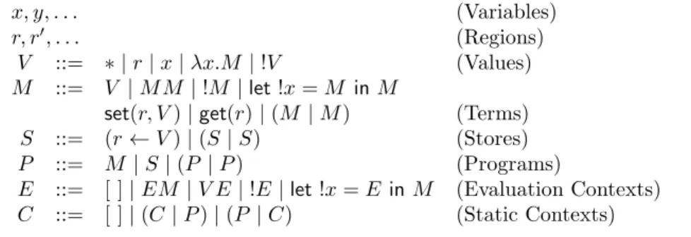
The syntax of the language is described in Table 3.1. We describe the new
x, y, . . . (Variables)
r, r′, . . . (Regions)
V ::= ∗ | r | x | λx.M | !V (Values)
M ::= V | M M | !M | let !x = M in M
set(r, V ) | get(r) | (M | M ) (Terms)
S ::= (r ← V ) | (S | S) (Stores)
P ::= M | S | (P | P ) (Programs)
E ::= [ ] | EM | V E | !E | let !x = E in M (Evaluation Contexts) C ::= [ ] | (C | P ) | (P | C) (Static Contexts)
Table 3.1: Syntax of programs: λ!R
operators. We have the usual set of variable x, y, . . . and a set of regions r, r′, . . ..
The set of values V contains the unit constant ∗, variables, regions, λ-abstraction and modal values !V which are marked with the bang operator ‘!’. The set of terms M contains values, application, modal terms !M , a let ! operator, set(r, V ) to write the value V at region r, get(r) to fetch a value from region r and (M | N ) to evaluate M and N in parallel. A store S is the composition of several stores (r ← V ) in parallel. A program P is a combination of terms and
stores. Evaluation contexts follow a call-by-value discipline. Static contexts C are composed of parallel compositions. Note that stores can only appear in a static context, thus M (M′ | (r ← V )) is not a legal term. We define
!n(P | P ) = (!nP | !nP ), and !n(r ← V ) = (r ← V ). As usual, we abbreviate
(λz.N )M with M ; N , where z is not free in N .
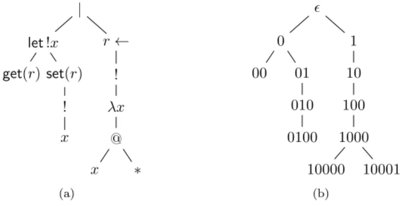
Each program has an abstract syntax tree as exemplified in Figure 3.1(a). | let!x get(r) set(r) ! x r ← ! λx @ x ∗ (a) ǫ 0 00 01 010 0100 1 10 100 1000 10000 10001 (b)
Figure 3.1: Syntax tree and addresses of P = let !x = get(r) in set(r, !x) | (r ← !(λx.x∗))
3.1.2 Operational Semantics
The operational semantics of the language is described in Table 3.2. Programs
P | P′ ≡ P′ | P (Commutativity) (P | P′) | P′′ ≡ P | (P′| P′′) (Associativity) E[(λx.M )V ] → E[M [V /x]] E[let !x = !V in M ] → E[M [V /x]] E[set(r, V )] → E[∗] | (r ← V ) E[get(r)] | (r ← V ) → E[V ]
E[let !x = get(r) in M ] | (r ← !V ) → E[M [V /x]] | (r ← !V ) Table 3.2: Semantics of λ!R programs
are considered up to a structural equivalence ≡ which is the least equivalence relation preserved by static contexts, and which contains the equations for α-renaming and for the commutativity and associativity of parallel composition. The reduction rules apply modulo structural equivalence and in a static context C.
When writing to a region, values are accumulated rather than overwritten (remember that λ!Ris an abstract language that can simulate more concrete ones
On the other hand, reading a region amounts to select non-deterministically one of the values associated with the region. We distinguish two rules to read a region. The first consumes the value from the store, like when reading a communication channel. The second copies the value from the store, like when reading a reference. Note that in this case the value read must be duplicable (of the shape !V ).
Example 3.1. Program P of Figure 3.1 reduces as follows: let!x = get(r) in set(r, !x) | (r ← !(λx.x∗)) → set(r, !(λx.x∗)) | (r ← !(λx.x∗))
→ ∗ | (r ← !(λx.x∗)) | (r ← !(λx.x∗))
3.2
Extended Depth System
We start by analysing the interaction between the depth of the occurrences and side effects. We observe that side effects may increase the depth or generate occurrences at lower depth than the current redex, which violates Property (1) and (2) (see Section 2.2) respectively. Then to find a suitable notion of depth, it is instructive to consider the following program examples where Mr= let !z =
get(r) in !(z∗).
(A) E[set(r, !V )] (B) λx.set(r, x); !get(r)
(C) !(Mr) | (r ← !(λy.Mr′)) | (r′ ← !(λy.∗))
(D) !(Mr) | (r ← !(λy.Mr))
(A) Suppose the occurrence set(r, !V ) is at depth δ > 0 in E. Then when evaluating such a term we always end up in a program of the shape E[∗] | (r ← !V ) where the occurrence !V , previously at depth δ, now appears at depth 0. This contradicts Property (2).
(B) If we apply this program to !V we obtain !!V , hence Property (1) is violated because from a program of depth 1, we reduce to a program of depth 2. We remark that this is because the read and write operations do not execute at the same depth.
(C) According to our definition, this program has depth 2, however when we reduce it we obtain a term !3∗ which has depth 3, hence Property (1) is
violated. This is because the occurrence λy.Mr′ originally at depth 1 in
the store, ends up at depth 2 in the place of z applied to ∗.
(D) If we accept circular stores, we can even write diverging programs whose depth is increased by 1 every two reduction steps.
Given these remarks, the rest of this section is devoted to a revised notion of depth and to depth system extended with side effects. First, we introduce the following contexts:
where δi is a natural number. We write dom(R) for the set {r1, . . . , rn}. We
write R(ri) for the depth δi associated with ri in the context R.
In the sequel, we shall call the notion of depth introduced in Definition 2.1 naive depth. We revisit the notion of naive depth as follows.
Definition 3.2(revised depth). Let P be a program, R a region context where dom(R) contains all the regions of P and dn(w) the naive depth of an occurrence
w of P . If w does not appear under an occurrence r ← (a store), then the revised depth dr(w) of w is dn(w). Otherwise, dr(w) is R(r)+dn(w). The revised depth
dr(P ) of the program is the maximum revised depth of its occurrences.
Note that the revised depth is relative to a fixed region context. In the sequel we write d( ) for dr( ). On functional terms, this notion of depth is equivalent
to the one given in Definition 2.1. However, if we consider the program of Figure 3.1, we now have d(10) = R(r) and d(100) = d(1000) = d(10000) = d(10001) = R(r) + 1.
A judgement in the depth system has the shape R; Γ ⊢δP and it should be interpreted as follows:
The free variables of !δP may only occur at the depth specified
by the context Γ, where depths are computed according to R.
The inference rules of the extended depth system are presented in Table 3.3. We comment on the new rules. A region and the constant ∗ may appear at
R; Γ, x : δ ⊢δ x R; Γ ⊢δ r R; Γ ⊢δ ∗ FO(x, M ) ≤ 1 R; Γ, x : δ ⊢δM R; Γ ⊢δλx.M R; Γ ⊢δ M i i = 1, 2 R; Γ ⊢δ M 1M2 R; Γ ⊢δ+1M R; Γ ⊢δ!M R; Γ ⊢δM 1 R; Γ, x : (δ + 1) ⊢δM2 R; Γ ⊢δlet!x = M 1inM2 R, r : δ; Γ ⊢δ get(r) R, r : δ; Γ ⊢δV R, r : δ; Γ ⊢δset(r, V ) R, r : δ; Γ ⊢δV R, r : δ; Γ ⊢0(r ← V ) R; Γ ⊢δ P i i = 1, 2 R; Γ ⊢δ(P 1| P2)
Table 3.3: Depth system for programs: λ!Rδ
any depth. The key cases are those of read and write: the depth of these two operations is specified by the region context. The current depth of a store is
always 0, however, the depth of the value in the store is specified by R (note that it corresponds to the revised definition of depth). We remark that R is constant in a judgement derivation.
Definition 3.3(well-formedness). A program P is well-formed if for some R, Γ, δ a judgement R; Γ ⊢δP can be derived.
Example 3.4. The program of Figure 3.1 is well-formed with the following derivation where R(r) = 0:
R; Γ ⊢0get(r)
R; Γ, x : 1 ⊢1x
R; Γ, x : 1 ⊢0!x R; Γ, x : 1 ⊢0set(r, !x)
R; Γ ⊢0let!x = get(r) in set(r, !x)
.. .
R; Γ ⊢0(r ← !(λx.x∗))
R; Γ ⊢0let!x = get(r) in set(r, !x) | (r ← !(λx.x∗))
We reconsider the troublesome programs with side effects. Program (A) is well-formed with judgement (i):
R; Γ ⊢0E[set(r, !V )] with R = r : δ (i)
R; Γ ⊢0!M
r| (r ← !(λy.Mr′)) | (r′← !(λy.∗)) with R = r : 1, r′ : 2 (ii)
Indeed, the occurrence !V is now preserved at depth δ in the store. Program (B) is not well-formed since the read operation requires R(r) = 1 and the write operations require R(r) = 0. Program (C) is well-formed with judgement (ii); indeed its depth does not increase anymore because !Mrhas depth 2 but since
R(r) = 1 and R(r′) = 2, (r ← !(λy.M
r′)) has depth 3 and (r′ ← !(λy.∗)) has
depth 2. Hence program (C) has already depth 3. Finally, it is worth noticing that the diverging program (D) is not well-formed since get(r) appears at depth 1 in !Mr and at depth 2 in the store.
Theorem 3.5(properties on the extended depth system). The following prop-erties hold:
1. If R; Γ ⊢δ M and x occurs free in M then x : δ′ belongs to Γ and all
occurrences ofx in !δM are at depth δ′.
2. If R; Γ ⊢δ P then R; Γ, Γ′⊢δ P .
3. If R; Γ, x : δ′⊢δM and R; Γ ⊢δ′
V then R; Γ ⊢δM [V /x] and
d(!δM [V /x]) ≤ max (d(!δM ), d(!δ′
V )).
4. If R; Γ ⊢0P and P → P′ thenR; Γ ⊢0P′ andd(P ) ≥ d(P′).
3.3
Elementary Bound
In this section, we prove that well-formed programs terminate in elementary time. The measure of Definition 2.5 extends trivially to programs except that
to simplify the proofs of the following properties, we assume the occurrences la-belled with | and r ← do not count in the measure and that set(r) counts for two occurrences such that the measure strictly decreases on the rule E[set(r, V )] → E[∗] | (r ← V ).
We derive a similar termination property:
Proposition 3.6 (termination). If P is well-formed, P → P′ and n ≥ d(P )
thenµn(P ) > µn(P′).
Proof. By a case analysis on the new reduction rules. • P ≡ E[set(r, V )] → P′ ≡ E[∗] | (r ← V )
If R; Γ ⊢δset(r, V ) then by 3.5(4) we have R; Γ ⊢0(r ← V ) with R(r) = δ.
Hence, by definition of the depth, the occurrences in V stay at depth δ in (r ← V ). However, the node set(r, V ) disappears, and both ∗ and (r ← V ) are null occurrences, thus ωδ(P′) = ωδ(P ) − 1. The number of occurrences
at other depths stay unchanged, hence µn(P ) > µn(P′).
• P ≡ E[get(r)] | (r ← V ) → P′ ≡ E[V ]
If R; Γ ⊢0 (r ← V ) with R(r) = δ, then get(r) must be at depth δ in
E[ ]. Hence, by definition of the depth, the occurrences in V stay at depth δ, while the node get(r) and | disappear. Thus ωδ(P′) = ωδ(P ) − 1
and the number of occurrences at other depths stay unchanged, hence µn(P ) > µn(P′).
• P ≡ E[let !x = get(r) in M ] | (r ← !V ) → P′ ≡ E[M [V /x]] | (r ← !V )
This case is the only source of duplication with the reduction rule on let !. Suppose R; Γ ⊢δ let!x = get(r) in M . Then we must have R; Γ ⊢δ+1 V .
The restrictions on the formation of terms require that x may only occur in M at depth 1 and hence in P at depth δ +1. Hence the occurrences in V stay at the same depth in M [V /x], while the let, get(r) and some x nodes disappear, hence ωδ(P ) ≤ ωδ(P′) − 2. The number of occurrences of x in
M is bound by k = ωδ+1(P ) ≥ 2. Thus if j > δ then ωj(P′) ≤ k · ωj(P ).
Clearly, ωj(M ) = ωj(M′) if j < i. Hence, we have
µn(P′) ≤ (µi+1n (P ) · k, ωi(P ) − 2, µi−1(P )) (3.1)
and µn(P ) > µn(P′).
Then we have the following theorem.
Theorem 3.7 (elementary bound). Let P be a well-formed program with α = d(P ) and let tαdenote the tower function withα+1 arguments. Then if P → P′
Proof. From the proof of termination, we remark that the only new rule that duplicates occurrences is the one that copies from the store. Moreover, the derived inequality (3.1) is exactly the same as the inequality (2.2). Hence the arithmetic of the proof is exactly the same as in the proof of elementary bound for the functional case.
Corollary 3.8. The normalisation of programs of bounded depth can be per-formed in time elementary in the size of the terms.
4
An Elementary Affine Type System
The depth system entails termination in elementary time but does not guarantee that programs ‘do not go wrong’. In particular, the introduction and elimination of bangs during evaluation may generate programs that deadlock, e.g.,
let!y = (λx.x) in !(yy) (4.1)
is well-formed but the evaluation is stuck. In this section we introduce an ele-mentary affine type system (λ!R
EA) that guarantees that programs cannot
dead-lock (except when trying to read an empty store).
The upper part of Table 4.1 introduces the syntax of types and contexts. Types are denoted with α, α′, . . .. Note that we distinguish a special behaviour
t, t′, . . . (Type variables)
α ::= B| A (Types)
A ::= t | 1 | A ⊸ α | !A | ∀t.A | RegrA (Value-types)
Γ ::= x1: (δ1, A1), . . . , xn: (δn, An) (Variable contexts) R ::= r1: (δ1, A1), . . . , rn : (δn, An) (Region contexts) R ↓ t R ↓ 1 R ↓ B R ↓ A R ↓ α R ↓ (A ⊸ α) R ↓ A R ↓ !A r : (δ, A) ∈ R R ↓ RegrA R ↓ A t /∈ R R ↓ ∀t.A ∀r : (δ, A) ∈ R R ↓ A R ⊢ R ⊢ R ↓ α R ⊢ α ∀x : (δ, A) ∈ Γ R ⊢ A R ⊢ Γ
Table 4.1: Types and contexts
to return a value (such as a store or several terms in parallel) while types of entities that may return a value are denoted with A. Among the types A, we distinguish type variables t, t′, . . ., a terminal type 1, an affine functional type
A ⊸ α, the type !A of terms of type A that can be duplicated, the type ∀t.A of polymorphic terms and the type RegrA of the region r containing values of
type A. Hereby types may depend on regions.
In contexts, natural numbers δi play the same role as in the depth system.
Writing x : (δ, A) means that the variable x ranges on values of type A and may occur at depth δ. Writing r : (δ, A) means that addresses related to region r contain values of type A and that read and writes on r may only happen at depth δ. The typing system will additionally guarantee that whenever we use a type RegrA the region context contains an hypothesis r : (δ, A).
Because types depend on regions, we have to be careful in stating in Table 4.1 when a region-context and a type are compatible (R ↓ α), when a region context is well-formed (R ⊢), when a type is well-formed in a region context (R ⊢ α) and when a context is well-formed in a region context (R ⊢ Γ). A more informal way to express the condition is to say that a judgement r1 : (δ1, A1), . . . , rn :
(δn, An) ⊢ α is well formed provided that: (1) all the region names occurring in
the types A1, . . . , An, α belong to the set {r1, . . . , rn}, (2) all types of the shape
RegriB with i ∈ {1, . . . , n} and occurring in the types A1, . . . , An, α are such
that B = Ai. We notice the following substitution property on types.
Proposition 4.1. IfR ⊢ ∀t.A and R ⊢ B then R ⊢ A[B/t].
Example 4.2. One may verify that r : (δ, 1 ⊸ 1) ⊢ Regr(1 ⊸ 1) can be
derived while the following judgements cannot: r : (δ, 1) ⊢ Regr(1 ⊸ 1), r :
(δ, Regr1) ⊢ 1.
A typing judgement takes the form: R; Γ ⊢δP : α
It attributes a type α to the program P at depth δ, in the region context R and the context Γ. Table 4.2 introduces an elementary affine type system with regions. One can see that the δ’s are treated as in the depth system. Note that a region r may occur at any depth. In the let ! rule, M should be of type !A since x of type A appears one level deeper. A program in parallel with a store should have the type of the program since we might be interested in the value the program reduces to; however, two programs in parallel cannot reduce to a single value, hence we give them a behaviour type. The polymorphic rules are straightforward where t /∈ (R; Γ) means t does not occur free in a type of R or Γ.
Example 4.3. The well-formed program (C) can be given the following typing judgement: R; ⊢0 !(M
r) | (r ← !(λy.Mr′)) | (r′ ← !(λy.∗)) : !!1 where:
R = r : (1, !(1 ⊸ 1)), r′ : (2, !(1 ⊸ 1)). Also, we remark that the deadlocking
R ⊢ Γ x : (δ, A) ∈ Γ R; Γ ⊢δ x : A R ⊢ Γ R; Γ ⊢δ ∗ : 1 R ⊢ Γ r : (δ′, A) ∈ R R; Γ ⊢δr : Reg rA FO(x, M ) ≤ 1 R; Γ, x : (δ, A) ⊢δM : α R; Γ ⊢δ λx.M : A ⊸ α R; Γ ⊢δ M : A ⊸ α R; Γ ⊢δ N : A R; Γ ⊢δ M N : α R; Γ ⊢δ+1M : A R; Γ ⊢δ !M : !A R; Γ ⊢δ M : !A R; Γ, x : (δ + 1, A) ⊢δ N : B R; Γ ⊢δ let!x = M in N : B R; Γ ⊢δM : A t /∈ (R; Γ) R; Γ ⊢δ M : ∀t.A R; Γ ⊢δ M : ∀t.A R ⊢ B R; Γ ⊢δ M : A[B/t] r : (δ, A) ∈ R R ⊢ Γ R; Γ ⊢δ get(r) : A r : (δ, A) ∈ R R; Γ ⊢δ V : A R; Γ ⊢δ set(r, V ) : 1 r : (δ, A) ∈ R R; Γ ⊢δV : A R; Γ ⊢0(r ← V ) : B R; Γ ⊢δP : α R; Γ ⊢δ S : B R; Γ ⊢δ (P | S) : α Pi not a store i = 1, 2 R; Γ ⊢δ P i: αi R; Γ ⊢δ(P 1| P2) : B
Table 4.2: An elementary affine type system: λ!R EA
Theorem 4.4(subject reduction and progress). The following properties hold. 1. (Well-formedness) Well-typed programs are well-formed.
2. (Weakening) If R; Γ ⊢δ P : α and R ⊢ Γ, Γ′ thenR; Γ, Γ′⊢δP : α.
3. (Substitution) If R; Γ, x : (δ′, A) ⊢δ M : α and R; Γ′ ⊢δ′
V : A and R ⊢ Γ, Γ′ thenR; Γ, Γ′⊢δ M [V /x] : α.
4. (Subject Reduction) If R; Γ ⊢δP : α and P → P′ then R; Γ ⊢δ P′: α.
5. (Progress) Suppose P is a closed typable program which cannot reduce. Then P is structurally equivalent to a program
M1| · · · | Mm| S1| · · · | Sn m, n ≥ 0
whereMi is either a value or can be decomposed as a termE[get(r)] such
5
Expressivity
In this section, we consider two results that illustrate the expressivity of the elementary affine type system. First we show that all elementary functions can be represented and second we develop an example of iterative program with side effects.
5.1
Completeness
The representation result just relies on the functional core of the language λ! EA.
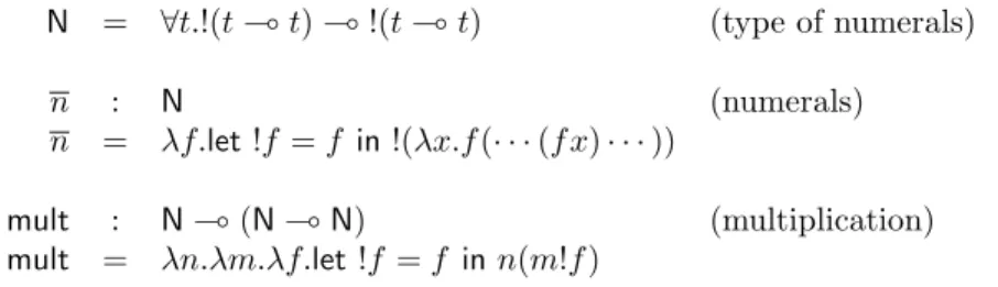
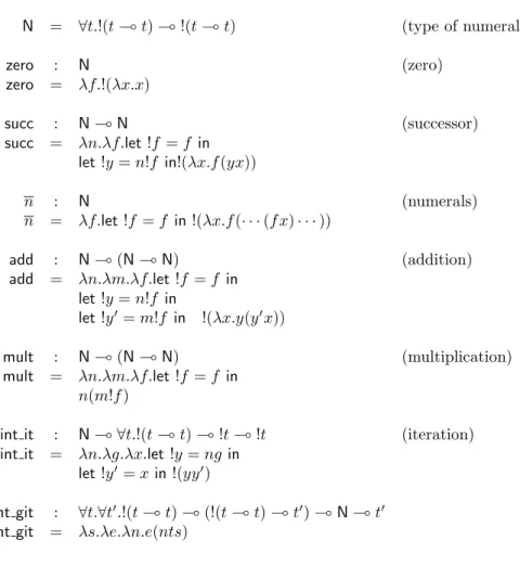
Building on the standard concept of Church numeral, Table 5.1 provides a repre-sentation for natural numbers and the multiplication function. We denote with
N = ∀t.!(t ⊸ t) ⊸ !(t ⊸ t) (type of numerals)
n : N (numerals)
n = λf.let !f = f in !(λx.f (· · · (f x) · · · ))
mult : N ⊸ (N ⊸ N) (multiplication)
mult = λn.λm.λf.let !f = f in n(m!f )
Table 5.1: Representation of natural numbers and the multiplication function Nthe set of natural numbers. The precise notion of representation is spelled out in the following definitions where by strong β-reduction we mean that reduction under λ’s is allowed.
Definition 5.1(number representation). Let ∅ ⊢δM : N. We say M represents
n ∈ N, written M n, if, by using a strong β-reduction relation, M→ n.∗ Definition 5.2 (function representation). Let ∅ ⊢δ F : (N
1 ⊸ . . . ⊸ Nk) ⊸
!pNwhere p ≥ 0 and f : Nk → N. We say F represents f , written F f , if
for all Mi and ni ∈ N where 1 ≤ i ≤ k such that ∅ ⊢δ Mi : N and Mi ni,
F M1. . . Mk f (n1, . . . , nk).
Elementary functions are also characterized as the smallest class of functions containing zero, successor, projection, subtraction and which is closed by com-position and bounded summation/product. These functions can be represented in the sense of Definition 5.2 by adapting the proofs from Danos and Joinet [10]. Theorem 5.3 (completeness). Every elementary function is representable in λ!
EA.
5.2
Iteration with Side Effects
We rely on a slightly modified language where reads, writes and stores relate to concrete addresses rather than to abstract regions. In particular, we introduce
terms of the form νx M to generate a fresh address name x whose scope is M . One can then write the following program:
νx ((λy.set(y, V ))x)→ νx ∗ | (x ← V )∗
where x and y relate to a region r, i.e. they are of type RegrA. Our type system
can be easily adapted by associating region types with the address names. Next we show that it is possible to program the iteration of operations producing a side effect on an inductive data structure. Specifically, in the following we show how to iterate, possibly in parallel, an update operation on a list of addresses of the store. The examples have been tested on a running implementation of the language.
Following Church encodings, we define the representation of lists and the associated iterator in Table 5.2. Here is the function multiplying the numeral
ListA = ∀t.!(A ⊸ t ⊸ t) ⊸ !(t ⊸ t) (type of lists)
[u1, . . . , un] : ListA (list represent.)
[u1, . . . , un] = λf.let !f = f in !(λx.f u1(f u2. . . (f unx))
list it : ∀u.∀t.!(u ⊸ t ⊸ t) ⊸ List u ⊸ !t ⊸ !t (iterator) list it = λf.λl.λz.let !z = z in let !y = lf in !(yz)
Table 5.2: Representation of lists pointed by an address at region r:
update : !RegrN ⊸ !1 ⊸ !1
update = λx.let !x = x in λz.!((λy.set(x, y))(mult 2 get(x)) Consider the following list of addresses and stores:
[!x, !y, !z] | (x ← m) | (y ← n) | (z ← p)
Note that the bang constructors are needed to match the type !RegrNof the
argument of update. Then we define the iteration as:
run: !!1 run= list it !update [!x, !y, !z] !!∗
Notice that it is well-typed with R = r : (2, N) since both the read and the write appear at depth 2. Finally, the program reduces by updating the store as expected:
run| (x ← m) | (y ← n) | (z ← p)
∗
→ !!1 | (x ← 2m) | (y ← 2n) | (z ← 2p)
Building on this example, suppose we want to write a program with three con-current threads where each thread multiplies by 2 the memory cells pointed by
a list. Here is a function waiting to apply a functional f to a value x in three concurrent threads:
gen threads : ∀t.∀t′
.!(t ⊸ t′
) ⊸ !t ⊸ B
gen threads = λf.let !f = f in λx.let !x = x in !(f x) | !(f x) | !(f x) We define the functional F as run but parametric in the list:
F : List !RegrN ⊸ !!1 F = λl.list it !update l !!∗
And the final term is simply:
run threads: B run threads= gen threads !F ![!x, !y, !z] where R = r : (3, !N). Our program then reduces as follows:
run threads | (x ← m) | (y ← n) | (z ← p)
∗
→ !!!1 | !!!1 | !!!1 | (x ← 8m) | (y ← 8n) | (z ← 8p)
Note that different thread interleavings are possible but in this particular case the reduction is confluent.
6
Conclusion
We have introduced a type system for a higher-order functional language with multithreading and side effects that guarantees termination in elementary time thus providing a significant extension of previous work that had focused on purely functional programs. In the proposed approach, the depth system plays a key role and allows for a relatively simple presentation. In particular we notice that we can dispense both with the notion of stratified region that arises in recent work on the termination of higher-order programs with side effects [1, 7] and with the distinction between affine and intuitionistic hypotheses [6, 2].
As a future work, we would like to adapt our approach to polynomial time. In another direction, one could ask if it is possible to program in a simplified language without bangs and then try to infer types or depths.
Acknowledgements We would like to thank Patrick Baillot for numerous helpful discussions and a careful reading on a draft version of this report.
References
[1] R. M. Amadio. On stratified regions. In APLAS’09, volume 5904 of LNCS, pages 210–225. Springer, 2009.
[2] R. M. Amadio, P. Baillot, and A. Madet. An affine-intuitionistic system of types and effects: confluence and termination. Technical report, Labora-toire PPS, 2009. http://hal.archives-ouvertes.fr/hal-00438101/.
[3] A. Asperti and L. Roversi. Intuitionistic light affine logic. ACM Trans. Comput. Log., 3(1):137–175, 2002.
[4] P. Baillot, M. Gaboardi, and V. Mogbil. A polytime functional language from light linear logic. In ESOP’10, volume 6012 of LNCS, pages 104–124. Springer, 2010.
[5] P. Baillot and K. Terui. A feasible algorithm for typing in elementary affine logic. In TLCA’05, volume 3461 of LNCS, pages 55–70. Springer, 2005. [6] A. Barber. Dual intuitionistic linear logic. Technical Report
ECS-LFCS-96-347, The Laboratory for Foundations of Computer Science, University of Edinburgh, 1996.
[7] G. Boudol. Typing termination in a higher-order concurrent imperative language. Inf. Comput., 208(6):716–736, 2010.
[8] P. Coppola, U. Dal Lago, and S. Ronchi Della Rocca. Light logics and the call-by-value lambda calculus. Logical Methods in Computer Science, 4(4), 2008.
[9] P. Coppola and S. Martini. Optimizing optimal reduction: A type inference algorithm for elementary affine logic. ACM Trans. Comput. Log., 7:219– 260, 2006.
[10] V. Danos and J.-B. Joinet. Linear logic and elementary time. Inf. Comput., 183(1):123 – 137, 2003.
[11] J.-Y. Girard. Light linear logic. Inf. Comput., 143(2):175–204, 1998. [12] U. D. Lago, S. Martini, and D. Sangiorgi. Light logics and higher-order
processes. In EXPRESS’10, volume 41 of EPTCS, pages 46–60, 2010. [13] K. Terui. Light affine lambda calculus and polynomial time strong
A
Proofs
A.1
Proof of theorem 3.5
1. We consider the last rule applied in the typing of M .
• Γ, x : δ ⊢δ x. The only free variable is x and indeed it is at depth δ
in !δx.
• Γ ⊢δ λy.M is derived from Γ, y : δ ⊢δ M . If x is free in λy.M then
x 6= y and x is free in M . By inductive hypothesis, x : δ′ ∈ Γ, y : δ
and all occurrences of x in !δM are at depth δ′. By definition of
depth, the same is true for !δ(λy.M ).
• Γ ⊢δ (M
1M2) is derived from Γ ⊢δ Mi for i = 1, 2. By inductive
hypothesis, x : δ′∈ Γ and all occurrences of x in !δM
i, i = 1, 2 are at
depth δ′. By definition of depth, the same is true for !δ(M 1M2).
• Γ ⊢δ!M is derived from Γ ⊢δ+1M . By inductive hypothesis, x : δ′∈
Γ and all occurrences of x in !δ+1M are at depth δ′ and notice that
!δ+1M = !δ(!M ).
• Γ ⊢δ let !y = M
1 in M2 is derived from Γ ⊢δ M1 and Γ, y : (δ +
1) ⊢δ M
2. Without loss of generality, assume x 6= y. By inductive
hypothesis, x : δ′ ∈ Γ and all occurrences of x in !δM
i, i = 1, 2 are
at depth δ′. By definition of depth, the same is true for !δ(let !y =
M1 inM2).
• M ≡ ∗ or M ≡ r or M ≡ get(r). There is no free variable in these terms.
• M ≡ let !y = get(r) in N . We have
R, r : δ; Γ, y : (δ + 1) ⊢δ N
R, r : δ; Γ ⊢δlet!y = get(r) in N
If x occurs free in M then x occurs free in N . By induction hypoth-esis, x : δ′ ∈ Γ and all occurrences of x in !δN are at depth δ′. By
definition of the depth, this is also true for !δ(let !y = get(r) in N ).
• M ≡ set(r, V ). We have
R, r : δ; Γ ⊢δ V
R, r : δ; Γ ⊢δ set(r, V )
If x occurs free in set(r, V ) then x occurs free in V . By induction hypothesis, x : δ′∈ Γ and all occurrences of x in !δV are at depth δ′.
By definition of the depth, this is also true for !δ(set(r, V )).
• M ≡ (M1| M2). We have
R; Γ ⊢δ M
i i = 1, 2
R; Γ ⊢δ (M 1| M2)
If x occurs free in M then x occurs free in Mi, i = 1, 2. By induction
hypothesis, x : δ′ ∈ Γ and all occurrences of x in !δM
i, i = 1, 2, are
at depth δ′. By definition of depth, the same is true of !δ(M 1| M2).
2. All the rules can be weakened by adding a context Γ′.
3. If x is not free in M , we just have to check that any proof of Γ, x : δ′⊢δ M
can be transformed into a proof of Γ ⊢δM .
So let us assume x is free in M .
We consider first the bound on the depth. By (1), we know that all occurrences of x in !δM are at depth δ′. By definition of depth, it follows
that δ′ ≥ δ and the occurrences of x in M are at depth (δ′ − δ). An
occurrence in !δ′
V at depth δ′+δ′′will generate an occurrence in !δM [V /x]
at the same depth δ + (δ′− δ) + δ′′.
Next, we proceed by induction on the derivation of Γ, x : δ′⊢δ M .
• Γ, x : δ ⊢δ x. Then δ = δ′, x[V /x] = V , and by hypothesis Γ ⊢δ′
V . • Γ, x : δ′⊢δλy.M is derived from Γ, x : δ′, y : δ ⊢δ M , with x 6= y and
y not occurring in N . By (2), Γ, y : δ ⊢δ′
V . By inductive hypothesis, Γ, y : δ ⊢δM [V /x], and then we conclude Γ ⊢δ(λy.M )[V /x].
• Γ, x : δ′ ⊢δ (M
1M2) is derived from Γ, x : δ′ ⊢δ Mi, for i = 1, 2. By
inductive hypothesis, Γ ⊢δM
i[V /x], for i = 1, 2 and then we conclude
Γ ⊢δ(M
1M2)[V /x].
• Γ, x : δ′ ⊢δ !M is derived from Γ, x : δ′ ⊢δ+1 M . By inductive
hypothesis, Γ ⊢δ+1M [V /x], and then we conclude Γ ⊢δ !M [V /x].
• Γ, x : δ′ ⊢δ let !y = M
1 in M2, with x 6= y and y not free in V is
derived from Γ, x : δ′ ⊢δ M
1 and Γ, x : δ′, y : (δ + 1) ⊢δ M2. By
inductive hypothesis, Γ ⊢δ M
1[V /x] Γ, y : (δ + 1) ⊢δ M2[V /x], and
then we conclude Γ ⊢δ (let !y = M
1in M2)[V /x].
• M ≡ let !y = get(r) in M1. We have
R, r : δ; Γ, x : δ′, y : (δ + 1) ⊢δ M 1
R, r : δ; Γ, x : δ′⊢δlet!y = get(r) in M 1
By induction hypothesis we get
R, r : δ; Γ, y : (δ + 1) ⊢δ M1[V /x]
and hence we derive
R, r : δ; Γ ⊢δ(let !y = get(r) in M1)[V /x]
• M ≡ set(r, V′). We have
R, r : δ; Γ, x : δ′ ⊢δV′
By induction hypothesis we get
R, r : δ; Γ ⊢δV′[V /x]
and hence we derive
R, r : δ; Γ ⊢δ(set(r, V′))[V /x] • M ≡ (M1| M2). We have R; Γ, x : δ′ ⊢δM i i = 1, 2 R; Γ, x : δ′ ⊢δ (M 1| M2)
By induction hypothesis we derive
R; Γ ⊢δ Mi[V /x]
and hence we derive
R; Γ ⊢δ (M
1| M2)[V /x]
4. We proceed by case analysis on the reduction rules.
• Suppose Γ ⊢0E[(λx.M )V ]. Then for some Γ′ extending Γ and δ ≥ 0
we must have Γ′⊢δ (λx.M )V . This must be derived from Γ′, x : δ ⊢δ
M and Γ′ ⊢δ V . By (3), with δ = δ′, it follows that Γ′ ⊢δ M [V /x]
and that the depth of an occurrence in E[M [V /x]] is bounded by the depth of an occurrence which is already in E[(λx.M )V ]. Moreover, we can derive Γ ⊢0E[M [V /x]].
• Suppose Γ ⊢0E[let !x = !V in M ]. Then for some Γ′extending Γ and
δ ≥ 0 we must have Γ′ ⊢δ let!x = !V in M . This must be derived
from Γ′, x : (δ + 1) ⊢δ M and Γ′⊢(δ+1)V . By (3), with (δ + 1) = δ′,
it follows that Γ′⊢δ M [V /x] and that the depth of an occurrence in
E[M [V /x]] is bounded by the depth of an occurrence which is already in E[let !x = !V in M ]. Moreover, we can derive Γ ⊢0E[M [V /x]].
• E[set(r, V )] → E[∗] | (r ← V )
We have R; Γ ⊢0E[set(r, V )] from which we derive
R; Γ ⊢δV
R; Γ ⊢δ set(r, V )
for some δ ≥ 0, with r : δ ∈ R. Hence we can derive R; Γ ⊢δV
R; Γ ⊢0(r ← V )
Moreover, we have as an axiom R; Γ ⊢δ ∗ thus we can derive R; Γ ⊢0
E[∗]. Applying the parallel rule we finally get R; Γ ⊢0E[∗] | (r ← V )
Concerning the depth bound, clearly we have d(E[∗] | (r ← V )) = d(E[set(r, V )]).
• E[get(r)] | (r ← V ) → E[M [V /x]]
We have R; Γ ⊢0E[get(r)] | (r ← V ) from which we derive
R; Γ ⊢δ get(r)
and
R; Γ, x : δ ⊢δ M
for some δ ≥ 0, with r : δ ∈ R, and R; Γ ⊢δV
R; Γ ⊢0(r ← V )
Hence we can derive
R; Γ ⊢0E[V ]
Concerning the depth bound, clearly we have d(E[V ]) = d(E[get(r)] | (r ← V )).
• E[let !x = get(r) in M ] | (r ← !V ) → E[M [V /x]] | (r ← !V )
We have R; Γ ⊢0E[let !x = get(r) in M ] | r!V from which we derive
R; Γ′, x : (δ + 1) ⊢δM
R; Γ′⊢δ let!x = get(r) in M
for some δ ≥ 0 with r : δ ∈ R, and some Γ′ extending Γ. We also
derive R; Γ ⊢δ+1V R; Γ ⊢δ!V R; Γ ⊢0(r ← !V ) By (2) we get R; Γ′⊢δ+1V . By (3) we derive R; Γ′⊢δ M [V /x] hence R; Γ ⊢0E[M [V /x]] and finally R; Γ ⊢0E[M [V /x]] | (r ← !V )
Concerning the depth bound, by (3), the depth of an occurrence in E[M [V /x]] | (r ← !V ) is bounded by the depth of an occur-rence which is already in E[let !x = get(r) in M ] | (r ← !V ), hence d(E[M [V /x]] | (r ← !V )) ≤ d(E[let !x = get(r) in M ] | (r ← !V )).
A.2
Proof of proposition 3.6
We do this by case analysis on the reduction rules. • P = E[(λx.M )V ] → P′= E[M [V /x]]
Let the occurrence of the redex (λx.M )V be at depth i. The restrictions on the formation of terms require that x occurs at most once in M at depth 0. Then ωi(P ) − 3 ≥ ωi(P′) because we remove the nodes for
application and λ-abstraction and either V disappears or the occurrence of the variable x in M disappears (both being at the same depth as the redex). Clearly ωj(P ) = ωj(P′) if j 6= i, hence
µn(P′) ≤ (ωn(P ), . . . , ωi+1(P ), ωi(P ) − 3, µi−1(P )) (A.1)
and µn(P ) > µn(P′).
• P = E[let !x =!V in M ] → P′ = E[M [V /x]]
Let the occurrence of the redex let !x =!V in M be at depth i. The restrictions on the formation of terms require that x may only occur in M at depth 1 and hence in P at depth i + 1. We have that ωi(P′) = ωi(P )− 2
because the let ! node disappear. Clearly, ωj(P ) = ωj(P′) if j < i. The
number of occurrences of x in M is bounded by k = ωi+1(P ) ≥ 2. Thus
if j > i then ωj(P′) ≤ k · ωj(P ). Let’s write, for 0 ≤ i ≤ n:
µi
n(P ) · k = (ωn(P ) · k, ωn−1(P ) · k, . . . , ωi(P ) · k)
Then we have
µn(P′) ≤ (µi+1n (P ) · k, ωi(P ) − 2, µi−1(P )) (A.2)
and finally µn(P ) > µn(P′).
• P ≡ E[set(r, V )] → P′ ≡ E[∗] | (r ← V )
If R; Γ ⊢δset(r, V ) then by 3.5(4) we have R; Γ ⊢0(r ← V ) with R(r) = δ.
Hence, by definition of the depth, the occurrences in V stay at depth δ in (r ← V ). Moreover, the node set(r, V ) disappears and the nodes ∗, |, and r ← appear. Recall that we assume the occurrences | and r ← do not count in the measure and that set(r) counts for two occurrences. Thus ωδ(P′) = ωδ(P )− 2 + 1 + 0 + 0. The number of occurrences at other depths
stay unchanged, hence µn(P ) > µn(P′).
• P ≡ E[get(r)] | (r ← V ) → P′ ≡ E[V ]
If R; Γ ⊢0 (r ← V ) with R(r) = δ, then get(r) must be at depth δ in
E[ ]. Hence, by definition of the depth, the occurrences in V stay at depth δ, while the node get(r) and | disappear. Thus ωδ(P′) = ωδ(P ) − 1
and the number of occurrences at other depths stay unchanged, hence µn(P ) > µn(P′).
• P ≡ E[let !x = get(r) in M ] | (r ← !V ) → P′ ≡ E[M [V /x]] | (r ← !V )
This case is the only source of duplication with the reduction rule on let !. Suppose R; Γ ⊢δ let!x = get(r) in M . Then we must have R; Γ ⊢δ+1 V .
The restrictions on the formation of terms require that x may only occur in M at depth 1 and hence in P at depth δ +1. Hence the occurrences in V stay at the same depth in M [V /x], while the let, get(r) and some x nodes disappear, hence ωδ(P ) ≤ ωδ(P′) − 2. The number of occurrences of x in
M is bounded by k = ωδ+1(P ) ≥ 2. Thus if j > δ then ωj(P′) ≤ k · ωj(P ).
Clearly, ωj(M ) = ωj(M′) if j < i. Hence, we have
µn(P′) ≤ (µi+1n (P ) · k, ωi(P ) − 2, µi−1(P )) (A.3)
and µn(P ) > µn(P′).
A.3
Proof of lemma 2.8
We start by remarking some basic inequalities.
Lemma A.1(some inequalities). The following properties hold on natural num-bers. 1. ∀ x ≥ 2, y ≥ 0 (y + 1) ≤ xy 2. ∀ x ≥ 2, y ≥ 0 (x · y) ≤ xy 3. ∀ x ≥ 2, y, z ≥ 0 (x · y)z≤ x(y·z) 4. ∀ x ≥ 2, y ≥ 0, z ≥ 1 xz· y ≤ x(y·z) 5. If x ≥ y ≥ 0 then (x − y)k ≤ (xk− yk)
Proof. 1. By induction on y. The case for y = 0 is clear. For the inductive case, we notice:
(y + 1) + 1 ≤ 2y+ 2y = 2y+1≤ xy+1 .
2. By induction on y. The case y = 0 is clear. For the inductive case, we notice:
x · (y + 1) ≤ x · (xy) (by (1))
= x(y+1)
3. By induction on z. The case z = 0 is clear. For the inductive case, we notice:
(x · y)z+1 = (x · y)z(x · y)
≤ xy·z(x · y) (by inductive hypothesis)
≤ xy·z(xy) (by (2))
4. From z ≥ 1 we derive y ≤ yz. Then:
xz· y ≤ xz· yz
= (x · y)z
≤ xy·z (by (3))
5. By the binomial law, we have xk= ((x − y) + y)k= (x − y)k+ yk+ p with
p ≥ 0. Thus (x − y)k= xk− yk− p which implies (x − y)k ≤ xk− yk.
We also need the following property.
Lemma A.2 (pre-shift). Assuming α ≥ 1 and β ≥ 2, the following property holds for the tower functions with x, x ranging over numbers greater or equal than2:
β · tα(x, x) ≤ tα(β · x, x)
Proof. This follows from:
β ≤ β2tα (x)
Then we can derive the proof of the shift lemma as follows. Let k = tα(x′, x) ≥ 2. Then
tα(β · x, x′, x) = β · (α · x)2
k
≤ (α · x)β·2k
(by lemma A.1(3)) ≤ (α · x)(β·2)k
≤ (α · x)2(β·k) (by lemma A.1(3))
and by lemma A.2 β · tα(x′, x) ≤ tα(β · x′, x).
Hence
(α · x)2(β·k) ≤ (α · x)2tα (β·x′,x)
= tα(x, β · x′, x)
A.4
Proof of theorem 3.7
Suppose µα(P ) = (x0, . . . , xα) so that xi corresponds to the occurrences at
depth (α − i) for 0 ≤ i ≤ α. Also assume the reduction is at depth (α − i). By looking at equations (A.1) and (A.2) in the proof of termination (Proposi-tion 3.6), we see that the components i + 1, . . . , α of µα(P ) and µα(P′) coincide.
Hence, let k = 2tα(xi+1,...,xα). By definition of the tower function, k ≥ 1.
We proceed by case analysis on the reduction rules. • P ≡ let !x = !V in M → P′≡ M [V /x]
By inequality (A.2) we know that:
tα(µα(P′)) ≤ tα(x0· xi−1, . . . , xi−1· xi−1, xi− 2, xi+1, . . . , xα)
By iterating lemma 2.8, we derive:
tα(x0· xi−1, x1· xi−1, . . . , xi−1· xi−1, xi− 2)
≤ tα(x0, x1· x2i−1, . . . , xi−1· xi−1, xi− 2)
≤ . . .
≤ tα(x0, x1, . . . , xii−1, xi− 2)
Renaming xi−1 with x and xi with y, we are left to show that:
(αxi)2(α·(y−2))k
< (αx)2(α·y)
k
Since i ≤ α the first quantity is bounded by: (αx)α·2(α·(y−2)) k We notice: α · 2(α·(y−2))k = α · 2(α·y−α·2)k ≤ α · 2(α·y)k−(α·2)k
(by lemma A.1(5)) So we are left to show that:
α2(α·y)k−(α·2)k)≤ 2(α·y)k Dividing by 2(α·y)k
and recalling that k ≥ 1, it remains to check: α · 2−(α·2)k≤ α · 2−(α·2)< 1
which is obviously true for α ≥ 1. • P ≡ (λx.M )V → P′≡ M [V /x]
By equation (A.1), we have that:
tα(µα(P′)) ≤ tα(x0, . . . , xi−1, xi− 2, xi+1, . . . , xα)
and one can check that this quantity is strictly less than: tα(µα(P )) = tα(x0, . . . , xi−1, xi, xi+1, . . . , xα)
• P ≡ let !x = get(r) in M | (r ← !V ) → P′≡ M [V /x] | (r ← !V )
Let k = 2tα(xi+1,...,xα). By definition of the tower function, k ≥ 1. By
equation (A.3) we have
tα(µα(P′)) ≤ tα(x0· xi−1, . . . , xi−1· xi−1, xi− 2, xi+1, . . . , xα)
= tα(x0· xi−1, . . . , xi−1· xi−1, xi− 2)k
• For the read that consume a value from the store, by looking at the proof of termination, we see that exactly one element of the vector µα(P ) is strictly
decreasing during the reduction, hence one can check that tα(µα(P )) >
tα(µα(P′)).
• The case for the write is similar to the read.
We conclude with the following remark that shows that the size of a program is proportional to its number of occurrences.
Remark A.3. The size of a program |P | of depth d is at most twice the sum of its occurrences: |P | ≤ 2 ·P
0≤i≤dωi(P ).
Hence the size of a program P is bounded by td(µd(P )).
A.5
Proof of proposition 4.1
By induction on A. • A ≡ t′
We have
R ⊢ t′ t /∈ R
R ⊢ ∀t.t′
If t 6= t′ we have t′[B/t] ≡ t′ hence R ⊢ [B/t]t′. If t ≡ t′ then we have
t′[B/t] ≡ B hence R ⊢ t′[B/t].
• A ≡ 1 We have
R ⊢ 1 t /∈ R R ⊢ ∀t.1 from which we deduce R ⊢ 1[B/t]. • A ≡ (C ⊸ D)
By induction hypothesis we have R ⊢ C[B/t] and R ⊢ D[B/t]. We then derive
R ⊢ C[B/t] R ⊢ D[B/t] R ⊢ (C ⊸ D)[B/t] • A ≡ !C
By induction hypothesis we have R ⊢ C[B/t], from which we deduce R ⊢ C[B/t] R ⊢ !C[B/t] • A ≡ RegrC We have R ⊢ r : C ∈ R R ⊢ RegrC t /∈ R R ⊢ ∀t.RegrC
As t /∈ R and r : (δ, C) ∈ R, we have r : (δ, C[B/t]) ∈ R, from which we deduce
R ⊢ r : (δ, C[B/t] ∈ R R ⊢ RegrC[B/t]
• A ≡ ∀t′.C
If t 6= t′: From R ⊢ ∀t.(∀t′.C) we have t′ ∈ R and by induction hypothesis/
we have R ⊢ C[B/t], from which we deduce R ⊢ C[B/t] t′∈ R/
R ⊢ (∀t′.C)[B/t]
If t ≡ t′ we have (∀t′.C)[B/t] ≡ ∀t′.C. Since we have
R ⊢ ∀t′.C t /∈ R
R ⊢ ∀t.(∀t′.C)
we conclude R ⊢ (∀t′.C)[B/t].
A.6
Proof of theorem 4.4
Properties 1 and 2 are easily checked. A.6.1 Substitution
If x is not free in M , we just have to check that any proof of Γ, x : (δ′, A) ⊢δ M
can be transformed into a proof of Γ ⊢δ M .
So let us assume x is free in M . Next, we proceed by induction on the derivation of Γ, x : δ′⊢δM .
• Γ, x : (δ, A) ⊢δ x : A. Then δ = δ′, x[V /x] = V , and by hypothesis
Γ ⊢δV : A.
• Γ, x : (δ′, A) ⊢δ λy.M : B ⊸ C is derived from Γ, x : (δ′, A), y : (δ, B) ⊢δ
M : C, with x 6= y and y not occurring in V . By (2), Γ, y : (δ, B) ⊢δ′
V : A. By inductive hypothesis, Γ, (y : δ, B) ⊢δ M [V /x] : C, and then we conclude
Γ ⊢δ(λy.M )[V /x] : B ⊸ C.
• Γ, x : (δ′, A) ⊢δ (M
1M2) : C is derived from Γ, x : (δ′, A) ⊢δ M1 : B ⊸
C and Γ, x : (δ′, A) ⊢δ M
1 : B ⊸ C. By inductive hypothesis, Γ ⊢δ
M1[V /x] : B ⊸ C and Γ ⊢δ M2[V /x] : C, and then we conclude Γ ⊢δ
(M1M2)[V /x] : C.
• Γ, x : (δ′, A) ⊢δ !M : !B is derived from Γ, x : (δ′, A) ⊢δ+1 M : B. By
inductive hypothesis, Γ ⊢δ+1 M [V /x] : B, and then we conclude Γ ⊢δ
!M [V /x] : !B.
• Γ, x : (δ′, A) ⊢δ let!y = M
1 in M2 : B, with x 6= y and y not free in V
is derived from Γ, x : (δ′, A) ⊢δ M
1: C and Γ, x : (δ′, A), y : (δ + 1, C) ⊢δ
M2 : B. By inductive hypothesis, Γ ⊢δ M1[V /x] : C Γ, y : (δ + 1, C) ⊢δ
• M ≡ get(r). We have R, r : (δ, B); Γ, x : (δ′, A) ⊢δ get(r) : B. Since
get(r)[V /x] = get(r) and x /∈ FV(get(r)) then R, r : (δ, B); Γ ⊢δget(r)[V /x] :
B.
• M ≡ set(r, V′). We have
R, r : (δ, C); Γ, x : (δ′, A) ⊢δ V′ : C
R, r : (δ, C); Γ, x : (δ′, A) ⊢δ set(r, V′) : 1
By induction hypothesis we get
R, r : (δ, C); Γ ⊢δ V′[V /x] : C
and hence we derive
R, r : (δ, C); Γ ⊢δ (set(r, V′))[V /x] : 1 • M ≡ (M1| M2). We have R; Γ, x : (δ′, A) ⊢δ M i: Ci i = 1, 2 R; Γ, x : (δ′, A) ⊢δ (M 1| M2) : B
By induction hypothesis we derive
R; Γ ⊢δ Mi[V /x] : Ci
and hence we derive
R; Γ ⊢δ (M1| M2)[V /x] : B
A.6.2 Subject Reduction
We first state and sketch the proof of 4 lemmas.
Lemma A.4 (structural equivalence preserves typing). If R; Γ ⊢δ P : α and
P ≡ P′ then R; Γ ⊢δ P′: α.
Proof. Recall that structural equivalence is the least equivalence relation in-duced by the equations stated in Table 3.2 and closed under static contexts. Then we proceed by induction on the proof of structural equivalence. This is is mainly a matter of reordering the pieces of the typing proof of P so as to obtain a typing proof of P′.
Lemma A.5 (evaluation contexts and typing). Suppose that in the proof of R; Γ ⊢δE[M ] : α we prove R; Γ′⊢δ′
M : α′. Then replacingM with a M′ such
thatR; Γ′⊢δ′
M′: α′, we can still derive R; Γ ⊢δE[M′] : α.
Lemma A.6 (functional redexes). If R; Γ ⊢δ E[∆] : α where ∆ has the shape
(λx.M )V or let !x = !V in M then R; Γ ⊢δE[M [V /x]] : α.
Proof. We appeal to the substitution lemma 3. This settles the case where the evaluation context E is trivial. If it is complex then we also need lemma A.5. Lemma A.7 (side effects redexes). If R; Γ ⊢δ ∆ : α where ∆ is one of the
programs on the left-hand side thenR; Γ ⊢δ ∆′: α where ∆′is the corresponding
program on the right-hand side:
(1) E[set(r, V )] E[∗] | (r ← V )
(2) E[get(r)] | (r ← V ) E[V ]
(3) E[let !x = get(r) in M ] | (r ← !V ) E[M [V /x]] | (r ← !V ) Proof. We proceed by case analysis.
1. Suppose we derive R; Γ ⊢δE[set(r, V )] : α from R; Γ′⊢δ′
set(r, V ) : 1. We can derive R; Γ′ ⊢δ′
∗ : 1 and by Lemma A.5 we derive R; Γ ⊢δ E[∗] : α
and finally R; Γ ⊢δ E[set(r, V )] | (r ← V ) : α.
2. Suppose R; Γ ⊢δ E[get(r)] : α is derived from R; Γ ⊢δ′
get(r) : A, where r : (δ′, A) ∈ R. Hence R; Γ ⊢0(r ← V ) : B is derived from R; Γ ⊢δ′
V : A. Finally, by Lemma A.5 we derive R; Γ ⊢δE[V ] : α.
3. Suppose R; Γ ⊢δ E[let !x = get(r) in M ] : α is derived from
R; Γ′ ⊢δ′
get(r) : !A R; Γ′, x : (δ′+ 1, A) ⊢δ′
M : α′
R; Γ′⊢δ′
let!x = get(r) in M : α′
where r : (δ′, !A) ∈ R. Hence R; Γ ⊢0 (r ← !V ) : B is derived from
R; Γ ⊢δ′+1
V : A. By Lemma 3 we can derive R; Γ′ ⊢δ′
M [V /x] : α′. Then
by Lemma A.5 we derive R; Γ ⊢δE[M [V /x]] : α.
We are then ready to prove subject reduction. We recall that P → P′ means
that P is structurally equivalent to a program C[∆] where C is a static context, ∆ is one of the programs on the left-hand side of the rewriting rules specified in Table 3.2, ∆′ is the respective program on the right-hand side, and P′ is
syntactically equal to C[∆′].
By lemma A.4, we know that R; Γ ⊢δ C[∆] : α. This entails that R′; Γ′⊢δ′
∆ : α′for suitable R′, Γ′, α′, δ′. By lemmas A.6 and A.7, we derive that R′; Γ′⊢δ′
∆′: α′. Then by induction on the structure of C we argue that R; Γ ⊢δC[∆′] : α.
A.6.3 Progress
To derive the progress property we first determine for each closed type A where A = A1 ⊸ A2 or A = !A1 the shape of a closed value of type A with the