The Effect of ENSO Shocks on Commodity Prices: A Multi-Time Scale Approach

HAL Id: halshs-03225070

https://halshs.archives-ouvertes.fr/halshs-03225070

Preprint submitted on 12 May 2021

HAL is a multi-disciplinary open access

archive for the deposit and dissemination of

sci-entific research documents, whether they are

pub-lished or not. The documents may come from

teaching and research institutions in France or

abroad, or from public or private research centers.

L’archive ouverte pluridisciplinaire HAL, est

destinée au dépôt et à la diffusion de documents

scientifiques de niveau recherche, publiés ou non,

émanant des établissements d’enseignement et de

recherche français ou étrangers, des laboratoires

publics ou privés.

The Effect of ENSO Shocks on Commodity Prices: A

Multi-Time Scale Approach

Gilles Dufrénot, William Ginn, Marc Pourroy

To cite this version:

Gilles Dufrénot, William Ginn, Marc Pourroy. The Effect of ENSO Shocks on Commodity Prices: A

Multi-Time Scale Approach. 2021. �halshs-03225070�

Working Papers / Documents de travail

WP 2021 - Nr 30

The Effect of ENSO Shocks on Commodity Prices:

A Multi-Time Scale Approach

Gilles Dufrénot

William Ginn

Marc Pourroy

The Effect of ENSO Shocks on Commodity Prices: A

Multi-Time Scale Approach

*

Gilles Dufr´enot

William Ginn

Marc Pourroy

May 11, 2021

Abstract

We investigate the effect of changing ENSO patterns on global commodity prices, including energy, metals/minerals and agriculture real commodity price subsets, while controlling for global economic out-put and interest rate via a global factor local projections (GFALP) model. We study the responses to climate shocks using a nonlinear multivariate model to assess differential effects across ENSO climate regimes. We find that commodity inflation is reactive to El Ni ˜no and La Ni ˜na events, but that this sensitivity can occur either in the short- or long-term depending on the commodity under investigation. For commodities in agriculture, we uncover an asymmetric influence of El Ni ˜no and La Ni ˜na shocks. More central banks are questioning whether climate change is part of their mission to stabilize prices. Our results indicate the ex-istence of a direct link between weather anomalies and commodity inflation, one that should be integrated into the central banks’ inflation targeting framework.

JEL Classification: C32, F44, O13, Q54.

Keywords: ENSO, Weather, Commodity Price, Agriculture, Energy.

*_{This work was supported by the French National Research Agency Grant ANR-17-EURE-0020, and by the Excellence Initiative of}

Aix-Marseille University - A*MIDEX.

†_{Aix-Marseille Univ, CNRS, AMSE, Marseille, France,Gilles.Dufrenot@univ-amu.fr} ‡_{Correspondance author, Adidas, Economist, Germany.William.Ginn.OBA@said.oxford.edu} §_{University of Poitiers, France.Marc.Pourroy@univ-poitiers.fr}

1

Introduction

Global climate is changing, and there is growing concern it increases the frequency and intensity of weather patterns (e.g.,Timmermann et al.(1999),Chen et al.(2001),An and Wang(2000)). Climate change poses serious threats to the core fabrics of our ecological, social and economic systems, yet the impact of changing climate is shrouded in uncertainty. Central to this concern is the effect on economic stability.

This paper explores the global dimensions of changing weather patterns and the international energy and agriculture commodity prices as they affect economic conditions. This research overlaps with two strands of literature. The first strand relates to a voluminous body of literature analyzing the effects that changing oil prices have on the macroeconomy (e.g.,Hamilton(1983),Hamilton(2008),Kilian(2009),Bodenstein et al.

(2011),Kilian(2014),Kang et al.(2017),Arouri et al.(2014),You et al.(2017), among others). Commodity prices (in real terms) tend to be endogenous and pro-cyclical to the global business cycle (e.g.,Kilian(2009),

Kilian and Zhou(2018)). Kilian(2009) distinguishes between demand and supply shocks in the oil price, and finds that increases in the oil price since 2003 are primarily driven by demand. The similar increases in the food price has raised concerns about inflationary pressures. This finding is also confirmed byJo¨ets et al.(2017) for corn, soybeans and wheat. This identification is consistent withAlquist and Kilian(2010), who finds that the oil price is determined endogenously and simultaneously.

The second strand relates to only a handful of papers to address the transmission that weather shocks has on economic conditions (Brunner(2002),Cashin et al.(2017),De Winne and Peersman(2018) andPeersman

(2018)).Brunner(2002) finds that weather shocks has important and statistically important effects on global commodity prices. Cashin et al. (2017) estimates a global vector autoregression to investigate weather shocks for twenty-one country/regions. Cashin et al. (2017) find heterogeneous responses of a weather shocks with regard to output growth.Peersman(2018) find that food price shocks can explain 30% inflation volatility in euro area.De Winne and Peersman(2018) show that increases in global agricultural commodity prices that are caused by unfavorable harvest shocks in other regions of the world can curtail domestic economic activity.

This paper provides three main contributions to the literature. First, using a rich dataset for nine economies representing circa two-thirds of global output1, we analyze to what extent a global El Ni ˜no weather and commodity price shock transmit a disturbance on the global factor economy. This paper is based on monthly data over the period 2002:04 to 2019:12, which has the potential benefit of capturing the short-term temporal effect that weather has on the economy (e.g.,Barnston(2015)), as opposed to using quarterly data as in previous studies (Brunner (2002), Cashin et al.(2017)). Most of the existing research climate change relates to disasters, which is primarily ex ante (Noy,2009), and mainly on prediction and prepara-tion (Cavallo and Noy,2009). This paper explores the transmission of changing ENSO weather conditions on agriculture, energy and metals/minerals price subsets, ex post.

Second, this paper employs a global factor augmented local projections model (GFALP) framework to as-sess the transmission of weather shocks on commodity, while controlling for global ouput, the interest rate and VIX. As the impact of El Ni ˜no or La Ni ˜na cannot be reduced to one country, but rather has global dimensions, this paper exploits a global factor model framework which paves the way to further our un-derstanding how changing ENSO climate patterns affect global commodity prices.

Third, of the rich literature that considers commodity prices, most papers include the oil price. This paper considers not only the energy price, which is more representative of the global economy than the oil price (Vasishtha and Maier,2013), but also the agriculture and metals/minerals price subsets. The global factor model approach further allows an identification such that agriculture, energy and metals/minerals prices are treated endogenously. An important benefit of this approach can be considered a structural extension toCashin et al.(2017), such that the authors treat oil and non-fuel commodities endogenous only to the US business cycle within a global VAR. Our model framework incorporates not only the effects of global ENSO

1_{The nine economies include: Canada (”CAN”), China (”CHN”), Euro zone (19 countries; ”EUR”), United Kingdom (”GBR”),}

India (”IND”), Japan (”JPN”), South Korea (”KOR”), Russia (”RUS”) and the United States (”USA”). Based on IMF data in pur-chasing power parity terms, the nine economies considered in this paper represent 66.1% of global output, seehttps://www.imf. org/external/datamapper/PPPSH@WEO/OEMDC/ADVEC/WEOWORLD/EU. The Euro zone values are based on the 19 member countries (i.e., Austria, Belgium, Cyprus, Estonia, Finland, France, Germany, Greece, Ireland, Italy, Latvia, Lithuania, Luxembourg, Malta, the Netherlands, Portugal, Slovakia, Slovenia, and Spain).

weather patterns, but also facilitates an endogenous treatment of commodity prices. This framework allows us to further inform our understanding of the consequential effects of changing ENSO weather patterns ex post, an area of paramount importance, considering current assessments of future climate scenarios are shrouded in uncertainty. Abril-Salcedo et al.(2020) looks at a non-linear relationship between ENSO and domestic Colombian food inflation. The closest paper to this research isUbilava(2018), who employs a TV-STAR model to estimate El Ni ˜no and La Ni ˜na weather patterns on global commodity prices.

Our paper differs from theirs on two crucial points.

First, we take into account the results from the rapidly expanding climate science literature which shows that changes in El Ni ˜no and La Ni ˜na operate in multiscale dimensions. Indeed, changes in climate system (temperature, precipitation, surface water pressure, etc) can be caused by changes in the structural mecha-nisms that govern the interdependencies of the components of this system. Such changes modify climatic regimes that must be differentiated from normal disturbances that are due to the stochastic nature of cer-tain climatic components. The multiscale approach then allows us to differentiate structural climate shocks from shocks whose effects dissipate rapidly. To do this, rather than estimating the smoothness parameter of the transition function, it is preferable to examine the response to shocks for different values of this pa-rameter. An advantage of this approach is that it allows to account for the diversity of responses observed historically in commodity inflation following El Ni ˜no and La Ni ˜na events. We know, for example, that from one region to another, these events have differentiated effects (positive or negative responses, small or big magnitudes) on countries’ GDP (see for exampleCashin et al.(2017)). Another advantage of looking at the effects of changing smoothness parameter is to facilitate possible counterfactual analysis.

Second, we use a multivariate framework. Indeed, not only are commodity markets interconnected, but El Ni ˜no and La Ni ˜na phenomena are weather shocks common to different commodities. A multivariate model has an advantage over the univariate models frequently used in the literature on commodity prices. It allows us to identify and estimate the true causal effects of climate change and to avoid over- or under-estimating their effects due to biases linked to omitted variables. For example, we know that the prices of many commodities are impacted by energy prices, hence the importance of studying simultaneously the dynamics of oil prices with those of other agricultural products and raw materials. We use the framework of a local projection model with a transition function, in order to differentiate the climate change regimes associated with cold or warm temperatures. In order to differentiate between the effects of climate varia-tions and those of other factors common to commodity price changes, we introduce other common factors, notably the international macro-financial environment that can influence price movements in international commodity markets: GDP and short term monetary policy rates in the world’s major industrialized and emerging countries. Another benefit of the local projections model framework is that the system does not necessarily remain static in a regime conditional that the system has entered the regime as in the smooth transition model byUbilava(2018).

Our paper highlights the fact that the impact of climate shocks can vary depending on the time scale at which they occur. These variations can concern the long-term components of the climate cycle, or the short-term components. Hence the importance of a multi-resolution analysis. We highlight this by showing the diversity of price responses to shocks for different values of the transition function parameter that measures temperature changes between warm (El Ni ˜no) and cold (La Ni ˜na) climate regimes. We find a significant influence of El Ni ˜no and La Ni ˜na events, considering both changes in the average levels of the indicators or in their extreme values (anomalies). Agricultural commodity prices appear to be more sensitive to climate variations reflecting changes in weather patterns than energy and non-energy commodity prices.

The rest of the paper is structured as follows: in Section 2 describes the data. Section 3 discusses the global dimensions of the business cycle considered in the paper. The modelling methodology and empirical results are summarized in Section 4. Section 5 concludes the paper.

2

Data

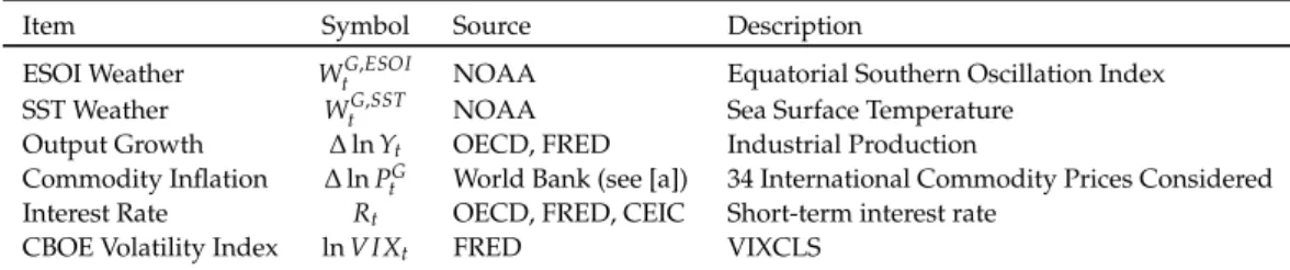
The GFALP model is based on the first principal component of nine economies covering output and the interest rate. The sample period is monthly which covers 2002:04 to 2019:12.2 The variables considered include a weather index via the Equatorial Southern Oscillation Index (ESOI) and Sea Surface Temperature (SST) index; industrial production index3; the short-term interest rate4; and 34 commodity prices. The data is summarized in Table 1.

Table 1: Variable Selection

Item Symbol Source Description

ESOI Weather W_tG,ESOI NOAA Equatorial Southern Oscillation Index

SST Weather WtG,SST NOAA Sea Surface Temperature

Output Growth ∆ ln Yt OECD, FRED Industrial Production

Commodity Inflation ∆ ln PG

t World Bank (see [a]) 34 International Commodity Prices Considered

Interest Rate Rt OECD, FRED, CEIC Short-term interest rate

CBOE Volatility Index ln V IXt FRED VIXCLS

[a]:https://www.worldbank.org/en/research/commodity-markets.

All variables are converted to logarithm with the exception of the interest rate and weather indices. The commodity price data, denominated in U.S. dollars, is deflated by dividing by the U.S. CPI. The ESOI and SST indices are used as a global measure of weather, which is collected from the National Oceanic and Atmospheric Administration (NOAA).

3

Global Dimensions of the Business Cycle

Three types of global variables are considered: two weather indices (ESOI and SST); global factors (output and interest rate); and 34 global commodity prices. Each are discussed in turn.

3.1

Global Weather Patterns

When a major El Ni ˜no (La Ni ˜na) occurs, there is an anomalous loss (increase) of heat from the ocean to at-mosphere so that global mean temperatures rise (fall) (McPhaden et al.,2020). The anomalous atmospheric patterns are known as the Southern Oscillation. El Ni ˜no, La Ni ˜na Southern Oscillation (ENSO) is one of the most important climate indicators, which has a major influence of global weather conditions (e.g., Ro-pelewski and Halpert(1987),Rosenzweig et al.(2001),McPhaden et al.(2006),Dai(2013) andBr ¨onnimann et al.(2007)).5

ENSO relates to cyclical, environmental conditions that occur across the equatorial Pacific Ocean. Changes to ENSO are due to natural interactions between sea surface temperature, rainfall, air pressure, atmospheric and oceanic circulation. The effects of ENSO, commonly called ”teleconnections”, emphasize that changing conditions can have a profound effect on global climate, which can in turn directly affect people’s liveli-hoods (e.g.,Barlow et al.(2001),Diaz et al.(2001), andAlexander et al.(2002)).

2_{The choice of economies and sample period combination is, in part, based on data availability. The sample period is quite}

extensive (213 observations per economy), while the nine economies considered represent the majority (66.12%) of global output at purchasing power parity using IMF data. The sample period also overlaps with the commodity price booms that occurred in 2004 (Radetzki,2006).

3_{For India, manufacturing production index (FRED mnemonic INDPRMNTO01IXOBM) is used as opposed to total production}

index (FRED mnemonic INDPROINDMISMEI), considering data availability (the correlation between the is 0.9918 for Jan 2000 to Dec 2018). For China, we use total production excluding construction (FRED mnemonic CHNPRINTO01IXPYM). As the production index for China includes missing values, the Kalman smoother using an ARIMA state space representation is used to impute missing values.

4_{For India, the interest rate is based on the 90 day Treasury Bill interest rate (e.g.,Patnaik et al.(2011),Gabriel et al.(2012),}

Saxegaard et al.(2010),Anand et al.(2014) andGinn and Pourroy(2020)).

5_{The NOAA considers ENSO as ”one of the most important climatic phenomena on Earth”, seehttps://www.weather.gov/mhx/}

Figure 1: Equatorial SOI Anomalies

While the Southern Oscillation Index (SOI), which is a commonly used indicator of ENSO, has been used in empirical papers as an indicator of weather as it relates to economic conditions (e.g.,Brunner(2002),Cashin et al.(2017)), the Equatorial Southern Oscillation Index (ESOI) is considered in this paper. According toShi and Su(2020), ESOI is superior to SOI since the former has a stronger correlation with the Ni ˜no 3.4 region sea surface temperature anomaly as well as with westerly/easterly wind bursts. Furthermore,Barnston

(2015) in a NOAA report suggests that ESOI overcomes two limitations of the SOI. First, SOI is based on the sea level pressure at just two stations (Tahiti and Darwin), which means ”it can be affected by shorter-term, day-to-day or week-to-week fluctuations unrelated to ENSO.” Second, the SOI is based on Tahiti and Darwin, both of which are located south of the equator whereas ”the ENSO phenomenon is focused more closely along the equator.” Taking these facts into consideration, the empirical analysis is based ESOI at monthly frequency (as opposed to quarterly data as inBrunner(2002) andCashin et al.(2017)). The ESOI is plotted in Figure 1, where blue (red) indicates La Ni ˜na (El Ni ˜no) conditions.

We also consider the Sea Surface Temperatures (SST) data, which is a 3-month running mean of sea surface temperature (SST) anomalies in the Ni ˜no 3.4 region that is above (below) the threshold of +0.5◦C (-0.5◦C). The SST is plotted in Figure 2, where blue (red) indicates La Ni ˜na (El Ni ˜no) conditions.

Figure 2: Sea Surface Temperature Anomalies

3.2

Global Factors

Following the approach byRatti and Vespignani(2016), we construct a global factor using the principal component indices for output and interest rate using normalized loadings. The benefit of this approach is that by taking the first principal component establishes a dimension reduction techniques that can replicate the main features of a global environment. The global factors represent nine economies which approximate two-thirds of global output using an extensive data from 2002:04 to 2019:12.

Y_tG = [Y_tCAN, Y_tCHN, Y_tEUR, Y_tGBR, YtI ND, YtJPN, YtKOR, YtRUS, YtUSA] (1)

We use one factor (the principal component) for the global variables (Ratti and Vespignani,2016). The results are provided in Table 2, which shows the top three principal components of each global variable for the nine economies. The first principle component captures significant share of the variance relating to output (54.9%) and the interest rate (54.1%).6

Figure 3 plots the global factors along with the economy data. The top-pane shows a sizable decline in output which occured during the global financial crisis.7

Table 2: Variation Explained by First Three Principal Components

Global Output Global Interest Rate

First Principal Component 54.9% 54.1%

Second Principal Component 33.5% 18.3%

Third Principal Component 6.4% 12.3%

Figure 3: Global Factors

The correlation between global variables (output and interest rate) is provided in Table 3. The correlation between global factor and country output is quite high for CAN, RUS and USA; and somewhat moderate for EUR and IND. There is lower correlation between the China and global output. The negative correlation between the UK and global output may be due to higher uncertainty in the UK related with Brexit. While it remains unclear to the extent that Brexit has had an impact on the domestic economy, a common thread is uncertainty, which has been linked with reduced investment, employment and productivity growth (Bloom et al.,2018).

6_{The higher dimensions of the principal components are provided in the Appendix, see the Scree plot in Figure 12. These values}

are similar toRatti and Vespignani(2016), where the first principle component in their paper captures for global output and interest rate represents 60.0% and 44.5% of the total variance, respectively.

Table 3: Correlation by Country and Global Variable

Country GLO CAN CHN EUR GBR IND JPN KOR RUS USA

Global Output 1.00 0.63 -0.81 0.51 -0.46 0.92 -0.1 0.91 0.98 0.81

Global Interest Rate 1.00 0.92 0.56 0.95 0.94 0.01 0.61 0.91 -0.25 0.81

3.3

Global Commodities

A total of 34 international commodities are analyzed in this study. The global factor model approach further allows an identification such that agriculture, energy and metals/minerals prices are treated endogenously. This allows us to analyze the effect that weather has on important commodity prices, while controlling for output, the interest rate and VIX.

Since the early 2000s, the world experienced elevated and persistent prices of many commodities relative to the somewhat more tranquil period after the mid-1980s. Several authors have dubbed this phenomena as a commodity price ”super cycle”.8 Hamilton(2008) motivates an argument of the importance of oil prices; that nine of ten recessions in the US since World War II have been preceded by an increase in oil prices. Yet the same argument can be conveyed for not only the broader set of energy prices, but also for metals/minerals and agriculture prices, at least since the turn of the century on a global scale at the onset of all four recessions (see Figure 4).9 Kilian and Vigfusson(2017) do not find evidence of a ”mechanical relationship” between an increase in the oil price and recessions.

Figure 4: International Energy and Agriculture Price

Source: World Bank (real terms). Indexed 2001:01 = 1. Shaded areas indicate OECD recession dates for 35 OECD member and non-member economies as proxy for global recession.

4

Weather shock identification

4.1

Multiple time scales in the oscillations of El Ni ˜no and La Ni ˜na

El Ni ˜no and La Ni ˜na phenomena result from nonlinear and complex interactions of the ocean-atmosphere system, implying that the succession of cool phases and warms phases of sea surface temperature are de-scribed by quasi-periodic fluctuations of different durations nested within each other. Geophysicists and climatologists explain the coexistence of quasi-periodic fluctuations by the interaction of different climatic subsystems (the physical and atmospheric factors that drive the different cycles are not necessarily identi-cal). Climate change can therefore be analyzed at different time scales. On the geological time scale, the time unit of measurement is the millennium. On the time scale of human activity, climate variations are described by the coexistence of long cycles lasting several decades, or 5 to 10 years, and shorter cycles of biennial, annual or infra-annual duration

8_{For example,Radetzki(2006) identifies the commodity price booms also occurred in the early 1950s, 1973/1974 and 2004 as the}

start of the third commodity price boom since the second world war.

9_{To illustrate this point, Figure 4 shows the international energy, metals/minerals and agriculture price movements against}

The durations of the cycles do not have the same effect on the transition phases between warming and cooling temperatures. Fluctuations of short duration involve very rapid transitions from one regime to the other, while fluctuations associated with cycles of longer duration have more persistent transition dynam-ics.

From a statistical point of view, a given observation of ESOI can be located on several cycles at the same time insofar as the fluctuations of different durations are nested. For example, a country may experience a cooling of temperatures by evolving in a state corresponding to La Ni ˜na on a cycle of short duration, while evolving at the same time in a phase of rising temperatures corresponding to El Ni ˜no on a cycle of longer duration. The impact of climate change on commodity inflation thus depends on the sensitivity of prices to each of these cycles.

To highlight the existence of multiple cycles in the dynamics of the ESOI series, a first approach is based on the estimation of long memory models. In their seminal paperBaillie and Chung(2002) show that annual temperature and width of tree ring time series data can be modelled by long-memory ARFIMA (autore-gressive fractionally integrated moving average) type models and that such models are consistent with temperature upward trend and global warming. More recently,Rypdal and Rypdal(2014) studied global warming from a system that includes the contribution of solar, volcanic, and anthropogenic activities and concludes that the system generates a long-memory temperature change process. Such studies are impor-tant, because it is known since the work byDiebold and Inoue(2001) that the presence of long-memory dynamics in time series are typical of processes subject to regime shifts. Using Northern hemisphere tem-perature data,Mills(2007) has shown that this applies in particular to climate data, where models with slowly changing levels and changes mimick long memory behavior.

The presence of cycles of long durations in the ESOI time series can be seen by estimating its spectrum (see Figure 5). Indeed, we observe important peaks of the spectral density in the vicinity of 0. The series thus includes long cycles. And these can mask the presence of short cycles. We estimate a Gegenbauer ARMA (GARMA) model, which is more general than the ARFIMA models usually used in the literature.

Figure 5: Spectrum of ESOI over 1949-2020

We estimate the following k-factor Gegenbauer process:

Φ(L)Πk_i=1(1−2ui+L2L)di(1−L)id(Xt−µ) =Θ(L)et (3)

where

• L is the lag operator defined by LjXt=Xt−j,

• Φ(L)is the short-memory autoregressive component of order p, • Θ(L)is is the short-memory moving average component of order q, • (1−2ui+L2L)di s the long-memory Gegenbauer component,

• id is the degree of integer differencing (here 0, • Xtis ESOI,

• etis an iid normal random component.

Our best model is obtained for p = q = 1, k = 3. The estimates in Table 4 suggest that the ESOI series has cycles that varies, with the longest cycle between 5 and 6 years (i.e., 67.88 months), followed by a cycle between 3 to 4 years (i.e., 42.99 months) and between 2 to 3 years (i.e. 29.47 months). The K-GARMA model has nevertheless several disadvantages. They are parametric models and therefore the number of factors that can be taken is limited by the non-linearity and the difficulties of convergence in the estimation of this type of model. This means that they do not capture all the cycles or quasi-fluctuations of the series. Moreover, long cycles can mask the presence of shorter cycles. An alternative is then to use non-parametric approaches.

Table 4: Estimate of a 3-factor GARMA model

Intercept u1 d1 u2 d2 u3 d3 ar1 ma1

Coefficient -0.0568 0.9957 0.1664 0.9893 0.1551 0.9773 0.1734 -0.3597 -0.1287

Standard Error 0.0011 0.0005 0.0021 0.0006 0.0007 0.0008 0.0011 0.0015 0.0028

Gegenbauer Factor1 Factor2 Factor3

Frequency: 0.0147 0.0233 0.0339

Period: 67.8793 42.9931 29.4697

Exponent: 0.1664 0.1551 0.1734

Wavelet analysis can be used to quantify ENSO variability. It is more general than Fourier-based transform and allows multiple time scale analysis. It has been successfully applied in the climatology literature (for a recent survey, the reader can refer toRhif et al.(2019)). We perform a multi-resolution decomposition by applying J-level wavelet filters to ESOI where J= {1, ..., 9}(Mallat decomposition). Low values of J capture high frequency components (short-term), while as J increases the decomposition filter low-frequency com-ponents (long-term). Figure 6 shows cycles of different lengths depending on the value of J (as an example, we have selected the graphs corresponding to J= {4, 5, 7, 8}).

Figure 6: ESOI Cycles Using Wavelet Decomposition

For J= 8, we observe long fluctuations with a modification of their duration in time. Until 1980, the ESOI series is negative for about ten years (El Ni ˜no regime), then positive for about 20 years (La Ni ˜na regime). From 1980, we observe a long El Ni ˜no regime that lasts almost 20 years, followed by an La Ni ˜na regime that lasts about the same duration.

For J=7 we see other quasi-periodic fluctuations of shorter length with average durations of the El Ni ˜no and La Ni ˜na regimes of about ten years. For J = {4, 5}, we observe quasi-periodic fluctuations of much shorter length corresponding to short-term climate variations.

The length of the fluctuations conditions the speed at which the transition from El Ni ˜no regime to La Ni ˜na regime takes place. We estimate the empirical distribution of each of the quasi-periodic fluctuations from the wavelet analysis (see Figure 7, for J= {1, 4, 5, 7}). These distributions have a sigmoidal shape. We note that as the value of J increases, the slope decreases. This suggests that as the length of the fluctuations in-creases, the time spent in a given regime becomes longer, which explains why the transition times between an El Ni ˜no regime and a La Ni ˜na regime are smoother.

Figure 7: ESOI cumulative distribution function for different time scales

We will now investigate the response of commodity inflation to ENSO shocks, taking into account that ENSO is composed of cycles of varying lengths embedded in each other. In addition to the fact that the response depends on the warming or cooling regimes, it varies depending on whether the shocks are persistent (because they belong to long quasi-cycles) or non-persistent (because they reflect the effect of short-term fluctuations.

4.2

Baseline Model

The local projections model with transition function, developed byJord`a(2005), is employed to estimate the dynamic responses that changing ENSO weather patterns have on commodity prices. In the benchmark specification, we estimate commodity inflation in real terms (πt) as follows:

πt+h =trendt+F(ζt−1)(αh,EN+φh,EN(L)xt−1+βh,ENshockt)+

(1−F(ζt−1))(αh,LN+φh,LN(L)xt−1+βh,LNshockt) +et+h (4)

which accounts for an asymmetry, which we define as an El Ni ˜no and La Ni ˜na climate state. F(ζt)is a

smooth transition function that represents the state of the climate: F(ζt) = exp (−γζt) 1+exp(−γζt) =1− 1 1+exp(−γζt), γ >0, |ζt|<∞. (5)

πt+his projected on the space generated by a set of control variables (xt−1). The vector of control variables

includes lags of the respective commodity price inflation, global output growth, global interest rate and VIX. In this specification, we allow the prediction of πt+h to differ according to the state of the climate

(i.e., in an El Ni ˜no and La Ni ˜na state) when a weather shock (shockt) occurs. The coefficient βh,EN (βh,LN)

corresponds with the estimated impact of the weather shock in a El Ni ˜no (La Ni ˜na) state.

ζtis a standardized transition variable and γ controls the degree of smoothness of the transition between

states. The transition variable is taken as ESOI. FollowingGorodnichenko and Auerbach(2013) andRamey and Zubairy(2018), the transition variable (ζt) is standardized by taking the cyclical component using the

Hodrick and Prescott (HP) filter.10 Consistent with Auerbach and Gorodnichenko(2012), the transition function is dated t−1 in Equation (9) to avoid contemporaneous feedback from policy actions with regard to the state of the economy (i.e., F(ζt−1)). For the baseline model, we consider γ=3, albeit we do consider

alternative values (which we describe in the next section).

When γ is large and ζt > 0, the logistic function F(ζt) approaches zero and the observed regime is La

Ni ˜na. When γ is large and ζt < 0, the ratio approaches 1, and the observed regime is El Ni ˜no. When γ is

large and ζtis near zero there is an indeterminate form (one can be in either one regime or the other). As

a consequence, when γ is large the logistic function behaves like an indicator function, thereby implying that any change from El Ni ˜no to La Ni ˜na regimes is instantaneous. In this case, we cannot differentiate the effect of climate shocks from a cold or warm temperature regime from the impulse response functions. The effects captured are therefore average effects.

When γ →0, the logistic function approaches a constant (1/2) and the models reduces to a linear model with a single regime.

When 0 < γ < ∞, the transition between the two regimes is more or less smooth and the responses to shocks occurring when temperatures are cold or warm can be differentiated.

With respect to the previous section, by varying the value of the γ coefficient, we consider the effect of climate variations corresponding to different time scales, i.e. the regime changes take place over cycles of different length. This is important because the different fluctuations ”overlap”, and we would like to know which cycles induce a change in commodity inflation during climate variations.

A caveat when we estimate the value of γ (rather than studying the impulse response function for dif-ferent values of this parameter) is that we are unable to know how much of the observed climate change comes from persistent shocks (because the changes occur on a cycle with a long length) and how much comes from non-persistent shocks (because they reflect short-term fluctuations). Changing the values γ is important because of the consequences for policies of resilience to climate shocks. Persistent shocks require structural resilience policies (improved storage conditions, changes in irrigation and water retention sys-tems to reduce the effects of possible droughts, adaptation of groundwater pumping strategies, etc). To limit the consequences of inflationary and deflationary effects of commodities linked to short-term climatic variations, policies that reduce income volatility may be more appropriate (hedging strategies, stabilization funds, etc).

The impulse response functions (IRF) and transition function for the model including the ESOI are sented in Figure 8. For robustness, the IRFs and transition function based on SST weather data are pre-sented in Figure 14. As there is serial correlation present in the error terms, the IRF plots include the 90% confidence band using the Newey West standard errors.

Figure 8: IRFs and Transition Function for ESOI on Commodity Prices

10_{The Hodrick-Prescott filter is applied using smoothing parameter λ = 129,600 (see e.g.Ravn and Uhlig(2002)), a standard value}

4.3

Sensitivity for varying γ

In Figure 9 we represent the impulse response functions for the three main types of commodities: agri-culture, energy, metals and minerals. The effects on the commodities that make up these three types are reported in the Appendix11. The occurrence of an El Ni ˜no event is interpreted as bringing high temperature, while the occurrence of La Ni ˜na is considered as bringing cold temperature.

The reading of the figures is as follows: what happens if we increase by one standard deviation -up or down depending on whether we are in an El Ni ˜no or La Ni ˜na regime- the value of ESOI? The effects of shocks are not significant when zero crosses the confidence interval.

For agriculture, we can clearly see the effect that changes in the γ coefficient have on IRFs. The difference between the confidence intervals narrows as the coefficient increases. The significance and duration of the shock response increases when changes in climate conditions capture long-term effects. For instance, when γ=0.1, prices rise or fall 6 months after the onset of an El Ni ˜no or La Ni ˜na shock and the effect lasts about 1 year (it fades after the 17th month). As the value of γ increases, the response to shocks occurs later and lasts for a very short time. One explanation for why agricultural commodity inflation are less sensitive to changes in climatic conditions occurring on short-term scales (larger γ values) is that changes in weather conditions are more predictable than structural changes and this facilitates the adoption of policies that are more resilient to shocks and thereby reduces the volatility of prices. We can see on the graph that the amplitude of the response is 10 times lower for γ>3 compared to γ=0.1.

The positive (resp. negative) response to the El Ni ˜no (resp. La Ni ˜na) shock is not compatible with the Cobweb theoretical model based on adaptive or rational expectations. Indeed, according to this model, a positive (resp. negative) shock should imply a cyclical dynamic of the response to shocks over time, which we do not observe here. Instead, the graphs suggest a positive autocorrelation in the responses to shocks, which is more compatible with the theoretical model of Laroque and Deaton (1996) where speculative behaviors increase autocorrelation and volatility in prices (such behaviors happen regularly in reality in times of significant temperature variations affecting agricultural yields).

The reaction of energy prices is different. For low values of γ, the price response is insignificant, while for values of the coefficient above 3, we have an immediate reaction with persistent price response over time. The response shows an S-shaped profile. It is significantly negative in the short term (up to 10 months), and then significantly positive from the 18thmonth onwards. Prices react in the same direction to both types of shocks (El Ni ˜no and La Ni ˜na).

The relationships between energy demand/supply and temperature changes are usually determined by composition effects resulting from geographical diversity (hot countries and cold countries), seasonal vari-ability, type of energy input and output (fuel, electricity, oil, coal,etc), heterogeneous household income level, or the average of cold and hot days. So, the global effects on international prices following changes in weather conditions can be either positive or negative. Our results are consistent with the following inter-pretations. Climate warming (temperature increase during El Ni ˜no, or decrease during La Ni ˜na) reduces the demand for heating fuel, thereby implying a fall in oil prices. On our graphs, if such an event happens, it does so in the short-run. But, on the other hand it also cause severe natural disasters such as floods or droughts which are likely to reduce production capacity in energy sector and thus drive energy prices to increase. The positive reaction is also consistent with the theoretical intertemporal CAPM model (ICAPM). According to our figures, if such events occur, they do so at long horizons (roughly 18 months after the initial shock).

The importance of the multivariate approach can be seen here because of the negative correlation between the responses of agricultural commodity prices and the responses of energy commodity prices. Indeed, an upsurge of El Ni ˜no events can lead to a decrease in agricultural production of different commodities such as wheat, soy, sugar, rice. When the phenomenon reaches the major producing countries in the world, the prices of agricultural commodities on international markets increase. However, the drop in agricultural production is synonymous with a decrease in exports from these countries (and therefore a drop in income), which leads to a constraint on the capacity to import energy products. The drop in demand can therefore

lead to a drop in the price of energy commodities. According to our figures, we observe both a positive reaction of agricultural commodities to El Ni ˜no shocks and a decrease in energy commodity prices. Our findings differ from some previous nonlinear weather-dependent energy models in the literature, and are in line with others. Moral-Carcedo and Vic´ens-Otero(2005) finds that the temperature-energy corre-lation is negative for the lowest temperatures, positive for the highest temperatures, but the link is less distinct for intermediate temperatures. In our case this would mean that the response should be asymmet-ric, which is not the case. Using a wavelet analysis,Qin et al.(2020) find that El Ni ˜no phenomenon has a negative impact on oil prices, but only in the long-run. Conversely,Cashin et al.(2017) find that El Ni ˜no phenomenon leads an increase in the oil prices in short-term, a reaction that can be explained by a higher demand from major industrialized and emergent economies such as the United States, Europe or China. For metals and minerals (non-energy), we find insignificant effects when γ is small, but significant defla-tionary pressure lasting 10 months after the shocks started when γ > 3. As with energy commodities, prices decreases for both El Ni ˜no and La Ni ˜na shocks.

Figure 9: IRFs and Transition Function for ESOI and Commodity Prices, Sensitivity to γ

Similar to Ubilava(2018), we estimate regime-dependent non-linearities of commodity price dynamics. Different from the author, we find it interesting to address the question: does an anomalous and a non-anomalous weather state matter, when an El Ni ˜no or La Ni ˜na condition enters into that state in relation to commodity inflation? To test this hypothesis, we employ a GFALP and further delineate between an anomalous (”A”) and non-anomalous (”NA”) regime, conditional on the ENSO type (i.e., El Ni ˜no and La Ni ˜na). We therefore relax the assumption of symmetry conditional on the weather shock. This allows us to assess whether the effect of an anomalous weather shock is asymmetric. Each regime-dependence model is discussed in turn.

We motivate this investigation with regard to the literature that is developing on the role of climate uncer-tainty on global commodity markets, the concept of unceruncer-tainty being associated with the extreme values of climate change indicators, i.e. when their values deviate too much from the average values (for a recent

example, seeNam(2021)). We use a threshold frequently chosen in the literature, i.e. that an anomaly exists as soon as the indicator exceeds 1 in absolute value.12

4.3.1 El Ni ˜no Anomalies Weather Conditions

To estimate whether an anomalies weather conditions matter in an El Ni ˜no state, Equation 9 is extended to include a latent variable and interaction terms:

πt+h =trendt+F(ζEN,A_t−1 )(αh,A+φh,A(L)xt−1+κh,A(xt−1×ItEN) +βh,A(shockt×ItEN) +γh,AItEN)+

(1−F(ζEN,A_t−1 ))(αh,N A+φh,N A(L)xt−1+κh,N A(xt−1×ItEN) +βh,N A(shockt×ItEN) +γh,N AItEN) +et+h

(6) where ζEN,A_t is a standardized transition variable and indicates an anomalous weather-dependent regime when an El Ni ˜no shock hits:

ζ_tEN,A= (

W_tG,ESOI, if W_tG,ESOI≤ −1

0, otherwise (7)

For an El Ni ˜no impact, we define an anomalous weather value as follows: ItEN =

(

1, if W_tG,ESOI<0

0, otherwise (8)

The IRFs and transition function plot for an El Ni ˜no regime-dependent model are presented in Figure 10.13 _{The IRFs indicate that while an anomalous weather shock has heterogenous effects by commodity,}

the magnitude of the weather shock in an anomalous state tends to be higher relative to a non-anomalous state. We highlight the following empirical findings:

• Agriculture: inflation is higher at the onset of the shock in an anomalous weather state. A closer inspection of the results shows that food commodities, particularly barley, beef, cocoa, grains, maize, sorghum and soybeans, are sensitive to an anomalous El Ni ˜no for most if not all periods. We also note that there is a lesser or even counter effect observed for banana (U.S. and Europe), chicken, and sugar prices in relation to anomalous weather. The effect on beverages is also inflationary on impact, where a non-anomalous weather impact emerges to cause higher inflation between periods 8 and 14. • Energy: inflation is higher at the onset of the shock in an anomalous weather state, whereas inflation in the non-anomalous state transition into marginally higher inflation approximately 9 months after the shock.

• Metals and Minerals: inflation is higher at the onset of the shock in an anomalous weather state, where a non-anomalous state evolves with higher inflation between periods 8 and 20. These results are fairly consistent for the individual metals and minerals commodities (i.e., natural gas, nickel, platinum, silver and gold).

Figure 10: IRFs and Transition Function for El Ni ˜no (ESOI) on Commodity Prices

12_{For Consistency with the baseline model, we keep γ=3 and λ=129, 600.} 13_{See Figure 16 in the Appendix for the IRFs by commodity price.}

4.3.2 La Ni ˜na Anomalous Weather Conditions

The model is similarly estimated for a La Ni ˜na shock:

π_t+h =trendt+F(ζLN,A_t−1 )(α_h,EN+φ_h,EN(L)xt−1+κ_h,LN(xt−1×ItLN) +βh,A(shockt×ItLN) +γh,AItLN)+

(1−F(ζ_t−1LN,A))(α_h,LN+φ_{h,N A}(L)xt−1+κ_{h,N A}(xt−1×ItLN) +βh,N A(shockt×ItLN) +γh,N AItLN) +et+h (9)

An anomalous La Ni ˜na weather shock is symmetrically defined as follows:

ζ_tLN,A= (

W_tG,ESOI, if W_tG,ESOI≥1

0, otherwise (10)

We define we define an anomalous La Ni ˜na weather value as follows: I_tLN=

(

1, if W_tG,ESOI >0

0, otherwise (11)

The IRFs and transition function plot for an La Ni ˜na regime-dependent model are presented in Figure 11.14 The IRFs indicate that while an anomalous weather shock has heterogenous effects by commodity, the magnitude of the weather shock in an anomalous state tends to be higher relative to a non-anomalous state. We highlight the following findings for an anomalous La Ni ˜na weather shock:

• Agriculture: inflation is higher in magnitude at the onset of the shock in an anomalous weather state. The effect is reasonably consistent for food and beverage commodities. The difference between an anomalous and non-anomalous weather state is less intense for food commodity in a La Ni ˜na event relative to an El Ni ˜no event.

• Energy: we do not observe major differences between inflation at the onset of the shock in an anoma-lous and non-anomaanoma-lous weather state, noting that inflation in the non-anomaanoma-lous state transitions into marginally higher inflation approximately 9 months after the shock.

• Metals and Minerals: inflation is higher in magnitude at the onset of the shock in an anomalous weather state, where a non-anomalous state evolves with higher inflation between periods 8 and 20. These results are fairly consistent for the individual metals and minerals commodities considered (i.e., natural gas, nickel, platinum, silver and gold).

Figure 11: IRFs and Transition Function for La Ni ˜na (ESOI) on Commodity Prices

5

Conclusion

This paper analyzes the global transmission of weather on commodity prices. We estimate a global factor augmented local projections model using a rich and extensive monthly data set from 2002:04 to 2019:12 relating to nine economies representing circa two-thirds of global output and 34 international commodity price sets.

We contribute to a narrow literature on the ”new climate economy” (Dell et al.,2014) in two ways. First, this paper exploits the global factor structure to investigate the global dimensions of weather and commodity

shocks. Second, we exploit the multivariate dimension of data using a nonlinear framework to account for possible changes in climate regimes.

We estimate a k-factor Gegenbauer ARMA process to isolate the multiple time scales in the oscillations of El Ni ˜no and La Ni ˜na states. We uncover the presence of cycles of various duration in the ESOI time series. What we observe at a given date is the combination of this set of cycles of different frequencies. Based on a Mallat decomposition, we are able to decompose and distinguish ESOI fluctuations as cycles of different lengths.

We then observe that the shape of the cumulative distribution function (CDF) is specific to each cycle: the longer the cycle, the smoother the CDF. A major contribution of our paper is that we later use this informa-tion on the CDF shape to calibrate the degree of smoothness of the transiinforma-tion funcinforma-tion of a local projecinforma-tions model. Therefore we can plot the IRFs on shocks associated to the different ENSO cycle frequencies. Assuming a low degree of smoothness of the transition function (γ) means that the model remains in a given state for longer periods of time, which corresponds to smooth CDF. Under this assumption (small γ), the estimated dynamic responses of a one standard deviation shock on ESOI has on agriculture commodities is strongly dependent on the ENSO regime: the agriculture commodity price reaction is positive (negative) during an El Ni ˜no (a La Ni ˜na) state. Interestingly energy, metal and minerals commodity price reaction is insignificant, meaning these commodities are not exposed to long cycle shocks.

A polar case for larger values of γ is associated with a faster transition from one state to another (El Ni ˜no / La Ni ˜na) and are therefore associated with shorter cycles. Under this calibration (high γ), the estimated dynamic impact of ESOI shocks on energy and metals and minerals commodities is strongly deflationary. Also, a key result is that agricultural commodity inflation is less sensitive to climatic conditions when considering short cycles than long cycles.

These results are relevant to understand the different challenges posed by climate change on commodities. Agricultural commodities are more impacted by shocks on long cycles than on short cycles. One possible explanation may be that agricultural production choices are long memory processes. As an example, we can think that in some regions of Latin America where potatoes have been grown for thousands of years, farmers will continue to grow them even if climate changes drastically. Changing this type of habits is extremely long as it calls for structural changes. Persistent shocks require structural resilience policies : improved storage conditions, changes in irrigation and water retention systems to reduce the effects of possible droughts, adaptation of groundwater pumping strategies, etc.

On the other hand, energy, metal and mineral commodities are more impacted by shocks on short cycles. These sectors being more capital intensive than agriculture, our results could reflect the ability of capital markets to shift investment in the medium run and therefore to avert from long run cycles shocks. Energy, metal and mineral commodities sensitivity to short cycle shocks could reflect both demand and supply conditions. To limit the consequences of inflationary and deflationary effects of commodities linked to short-term climatic variations, policies that reduce income volatility may be more appropriate (hedging strategies, stabilization funds, etc).

Climate change can be seen both as a change in long term trend and a change in the distribution of shocks, which could lead to a potential increase of extreme events. We therefore find it interesting to investigate whether commodities react to anomalous weather conditions. Using a local projections model, we show that the distinction between anomalies and standard conditions matter in the transmission of weather shocks to commodities: an anomalous El Ni ˜no weather shock leads to higher inflation at the onset of the shock for all three categories (agriculture, energy, metals and minerals commodities). Similarly, an anoma-lous La Ni ˜na weather shock leads to higher inflation at the onset of the shock (with the exception of energy). This result is particularly relevant as it highlights how climate change, if defined as more frequent extreme events, could impact financial markets via the valuation of commodities. More broadly, as commodity price pass through to consumer prices, this result shows how an increase of extreme events could impact the whole economy through the price channel. More central banks are questioning whether climate change is part of their mission to stabilize prices (seeNGSF(2021)). Our results indicate the existence of a direct link between weather anomalies and commodity inflation, one that should be integrated into the inflation targeting framework.

The results from this research have both immediate and long-term policy implications regarding the adap-tation to climate changes. A starting point for short-term policy is to establish sources of vulnerability that could create economic risks. The findings from this paper serve to do just that in a global factor environment by analyzing the propagation mechanisms through which weather shocks influence commodity inflation. These insights are of paramount importance to central bank policies designed to understand sources of price changes to stabilize agriculture and aggregate prices, inter alia. Similarly fiscal policy is subject to endogenous policy responses to smooth household consumption via food subsidy program.

Over the longer term, policy makers should address the adaptation with regard to climate change. Policy needs to address changes to the social and economic systems from multiple fronts. The central bank must craft an appropriate policy response that monitors and addresses sectoral price developments as they relate to the changing business cycle and the effects of climate change. This is of growing importance as climate change is expected to increase the frequency and intensity of weather patterns (e.g.,Timmermann et al.

(1999),Chen et al.(2001),An and Wang(2000)). The impact of climate change may influence the central bank’s interest rate, which can in turn influence the stock market and investment decisions. Overlooking the effects of changing weather patterns has on future inflation could potentially move inflation away from central bank’s target, thereby weakening central bank’s monetary anchoring. Similarly, a weather shock that results in higher food prices may create a source of vulnerability with regards to a combination of debt and taxes needed to finance food subsidies.

6

Bibliography

Abril-Salcedo, D. S., Melo-Velandia, L., and Parra-Amado, D. (2020). Nonlinear relationship between the weather phenomenon El Eino and Colombian food prices. Australian Journal of Agricultural and Resource Economics, 64(4):1059–1086.

Alexander, M., Blad´e, I., Newman, M., Lanzante, J., Lau, N.-C., and Scott, J. (2002). The atmospheric bridge: The influence of ENSO teleconnections on air–sea interaction over the global oceans. Journal of Climate, 15(16):2205–2231.

Alquist, R. and Kilian, L. (2010). What do we learn from the price of crude oil futures? Journal of Applied Econometrics, 25(4):539–573.

An, S.-I. and Wang, B. (2000). Interdecadal change of the structure of the ENSO mode and its impact on the ENSO frequency. Journal of Climate, 13(12):2044–2055.

Anand, R., Ding, D., and Tulin, V. (2014). Food inflation in India: the role for monetary policy. Number 14-178. International Monetary Fund.

Arouri, M., Rault, C., and Teulon, F. (2014). Economic policy uncertainty, oil price shocks and GCC stock markets. Economics Bulletin, 34(3):1822–1834.

Auerbach, A. J. and Gorodnichenko, Y. (2012). Measuring the output responses to fiscal policy. American Economic Journal: Economic Policy, 4(2):1–27.

Baillie, Richard, T. and Chung, S.-K. (2002). Modelling and forecasting from trend-stationary long-memory models with applications to climatology. International Journal of Forecasting, 18(2):215–226.

Barlow, M., Nigam, S., and Berbery, E. (2001). ENSO, pacific decadal variability, and US summertime precipitation, drought, and stream flow. Journal of Climate, 14(9):2105–2128.

Barnston, A. (2015). Why are there so many ENSO indexes, instead of just one. NOAA Climate. gov. Bloom, N., Chen, J., and Mizen, P. (2018). Rising Brexit uncertainty has reduced investment and

employ-ment. VOX CEPR policy portal, 16.

Bodenstein, M., Erceg, C., and Guerrieri, L. (2011). Oil shocks and external adjustment. Journal of International Economics, 83(2):168–184.

Br ¨onnimann, S., Xoplaki, E., Casty, C., Pauling, A., and Luterbacher, J. (2007). ENSO influence on Europe during the last centuries. Climate Dynamics, 28(2-3):181–197.

Brunner, A. D. (2002). El nino and world primary commodity prices: warm water or hot air? Review of Economics and Statistics, 84(1):176–183.

Cashin, P., Mohaddes, K., and Raissi, M. (2017). Fair weather or foul? The macroeconomic effects of El Ni ˜no. Journal of International Economics, 106:37–54.

Cavallo, E. A. and Noy, I. (2009). The economics of natural disasters: a survey. Inter-American Development Bank.

Chen, C., McCarl, B., and Adams, R. (2001). Economic implications of potential ENSO frequency and strength shifts. Climatic Change, 49(1):147–159.

Dai, A. (2013). Increasing drought under global warming in observations and models. Nature Climate Change, 3(1):52–58.

De Winne, J. and Peersman, G. (2018). Agricultural price shocks and business cycles-a global warning for advanced economies.

Dell, M., Jones, B. F., and Olken, B. A. (2014). What do we learn from the weather? The new climate-economy literature. Journal of Economic Literature, 52(3):740–98.

Diaz, H. F., Hoerling, M. P., and Eischeid, J. K. (2001). ENSO variability, teleconnections and climate change. International Journal of Climatology: A Journal of the Royal Meteorological Society, 21(15):1845–1862. Diebold, F. X. and Inoue, A. (2001). Long memory and regime switching. Journal of Econometrics, 105:139–

159.

Gabriel, V., Levine, P., Pearlman, J., and Yang, B. (2012). An Estimated DSGE Model of the Indian Economy, The Oxford Handbook of the Indian Economy, (Ed). Chetan Ghate. Oxford University Press.

Ginn, W. and Pourroy, M. (2020). The contribution of food subsidy policy to monetary policy.

Gorodnichenko, Y. and Auerbach, A. J. (2013). Fiscal Multipliers in Recession and Expansion. University of Chicago Press.

Hamilton, J. (1983). Oil and the macroeconomy since World War II. Journal of Political Economy, 91(2):228– 248.

Hamilton, J. (2008). Oil and the macroeconomy. The New Palgrave Dictionary of Economics, 2.

Jo¨ets, M., Mignon, V., and Razafindrabe, T. (2017). Does the volatility of commodity prices reflect macroe-conomic uncertainty? Energy Emacroe-conomics, 68:313–326.

Jord`a, `O. (2005). Estimation and inference of impulse responses by local projections. American Economic Review, 95(1):161–182.

Kang, W., de Gracia, F., and Ratti, R. (2017). Oil price shocks, policy uncertainty, and stock returns of oil and gas corporations. Journal of International Money and Finance, 70:344–359.

Kilian, L. (2009). Not all oil price shocks are alike: Disentangling demand and supply shocks in the crude oil market. American Economic Review, 99(3):1053–69.

Kilian, L. (2014). Oil price shocks: Causes and consequences.

Kilian, L. and Vigfusson, R. (2017). The role of oil price shocks in causing US recessions. Journal of Money, Credit and Banking, 49(8):1747–1776.

Kilian, L. and Zhou, X. (2018). Modeling fluctuations in the global demand for commodities. Journal of International Money and Finance, 88:54–78.

Laroque, G. and Deaton, A. (1996). Competitive storage and commodity price dynamics. Journal of Political Economy, 104(5):896–923.

McPhaden, M., Santoso, A., and Cai, W. (2020). Introduction to El Ni ˜no southern oscillation in a changing climate. El Ni ˜no Southern Oscillation in a Changing Climate, pages 1–19.

McPhaden, M., Zebiak, S., and Glantz, M. (2006). ENSO as an integrating concept in earth science. Science, 314(5806):1740–1745.

Mills, T. C. (2007). Time series modelling of two millennia of northern hemisphere temperatures: long mem-ory or shifting trends? Journal of The Royal Statistical Society, Statistics in Society Series A, 170(1):83–94. Moral-Carcedo, J. and Vic´ens-Otero, J. (2005). Measuring the output responses to fiscal policy. Energy

Economics, 27(3):477–494.

Nam, K. (2021). Investigating the effect of climate uncertainty on global commodity markets. Energy Economics, 96(3):105–123.

NGSF (2021). Adapting central bank operations to a hotter world. reviewig some options. Technical docu-ment, Network for Greening the Financial System.

Noy, I. (2009). The macroeconomic consequences of disasters. Journal of Development economics, 88(2):221–231.

Patnaik, I., Shah, A., and Bhattacharya, R. (2011). Monetary policy transmission in an emerging market setting. Number 11-15. International Monetary Fund.

Peersman, G. (2018). International food commodity prices and missing (dis) inflation in the euro area. Qin, M., Qiu, L.-H., Tao, R., Umar, M., Su, C.-W., and Jiao, W. (2020). The inevitable role of El Ni ˜no: a fresh

insight into the oil market. Economic Research-Ekonomska Istraˇzivanja, 33(1):1943–1962. Radetzki, M. (2006). The anatomy of three commodity booms. Resources Policy, 31(1):56–64.

Ramey, V. and Zubairy, S. (2018). Government spending multipliers in good times and in bad: evidence from US historical data. Journal of Political Economy, 126(2):850–901.

Ratti, R. A. and Vespignani, J. L. (2016). Oil prices and global factor macroeconomic variables. Energy Economics, 59:198–212.

Ravn, M. and Uhlig, H. (2002). On adjusting the Hodrick-Prescott filter for the frequency of observations. Review of Economics and Statistics, 84(2):371–376.

Rhif, M., Ben Abbes, A., Farah, I. R., Mart´ınez, B., and Sang, Y. (2019). Wavelet transform application for/in non-stationary time-series analysis: a review. Applied Sciences, 9(7):1345.

Ropelewski, C. and Halpert, M. (1987). Global and regional scale precipitation patterns associated with the El Ni ˜no/Southern Oscillation. Monthly Weather Review, 115(8):1606–1626.

Rosenzweig, C., Iglesias, A., Yang, X., Epstein, P., and Chivian, E. (2001). Climate change and extreme weather events. Global Change and Human Health, 2(2):90.

Rypdal, M. and Rypdal, K. (2014). Long-memory effects in linear response models of earth’s temperature and implications for future global warming. Journal of Climate, 27(14):5240–5258.

Saxegaard, M., Anand, R., and Peiris, S. (2010). An estimated model with macrofinancial linkages for India. Number 10-21. International Monetary Fund.

Shi, Y. and Su, J. (2020). A new equatorial oscillation index for better describing ENSO and westerly wind bursts. Journal of Meteorological Research, 34(5):1025–1037.

Timmermann, A., Oberhuber, J., Bacher, A., Esch, M., Latif, M., and Roeckner, E. (1999). Increased El Ni ˜no frequency in a climate model forced by future greenhouse warming. Nature, 398(6729):694–697.

Ubilava, D. (2018). The role of el nino southern oscillation in commodity price movement and predictability. American Journal of Agricultural Economics, 100(1):239–263.

Vasishtha, G. and Maier, P. (2013). The impact of the global business cycle on small open economies: A FAVAR approach for Canada. The North American Journal of Economics and Finance, 24:191–207. You, W., Guo, Y., Zhu, H., and Tang, Y. (2017). Oil price shocks, economic policy uncertainty and industry

7

Appendix

7.1

Scree Plots

The scree plots are provided for the global factor analysis of output and interest rate. The scree plot is a plot of the eigenvalues of principal components.

7.2

Additional IRFs

We provide additional IRFs (referenced and described in the main text).