Capacity control in network revenue management : clustering and risk-aversion

Capacity control in network revenue management:

Clustering and risk-aversion

by

Joongwoo Brian Park

B.S. in Electrical Engineering and Computer Science

Korea Advanced Institute of Science and Technology, 2007

Submitted to the Department of Electrical Engineering and Computer

Science

in partial fulfillment of the requirements for the degree of

Master of Science in Electrical Engineering and Computer Science

at the

MASSACHUSETTS INSTITUTE OF TECHNOLOGY

February 2010

@

Massachusetts Institute of Technology 2010. All rights reserved.

ARCHfVES

Author ...

Dy tmet(of Electrical Engineering and Computer Science

December 31, 2009

Certified by. .

_...

Vivek F. Farias

Robert N. Noyce Career Development Assistant Professor in Sloan

School of Management

Thesis Supervisor

A ccepted by ...

...

Terry Orlando

Chairman, Department Committee on Graduate Students

MASSACHUSETTS INSt UTE OF TECHNOLOGY

FEB 2

3

2010

Capacity control in network revenue management:

Clustering and risk-aversion

by

Joongwoo Brian Park

Submitted to the Department of Electrical Engineering and Computer Science on December 31, 2009, in partial fulfillment of the

requirements for the degree of

Master of Science in Electrical Engineering and Computer Science

Abstract

Network revenue management is the practice of using optimal decision policies to increase revenues by controlling limited quantities of multiple resources' availability and prices over finite time. It is widely practiced in capacity-constrained service industries such as the airlines, hotels, car rentals, and cruise-lines. A variety of control methods has been introduced for network resource capacity control problem. We propose a clustering method to improve approximation quality. By clustering the legs of the network, one can find tighter upperbound than leg-wise decomposition with loss of computation speed due to larger state space. We have shown that there is more than 6% revenue improvement opportunity by finding the right clustering. With local interchange heuristic and generic heuristics, finding a locally optimal clustering can be done in faster time. We also introduce risk-aversion in network revenue management. We have investigated risk-aversion on network revenue management and also study the impact of risk-aversion parameters in the optimization model on relative revenue-risk performance.

Thesis Supervisor: Vivek F. Farias

Title: Robert N. Noyce Career Development Assistant Professor in Sloan School of Management

Acknowledgments

I have made many important choices over the past few years; indeed, one of the best

choice I have made is to work with Professor Vivek Farias. I am so grateful that he allowed me much freedom in pursuing my own ideas, while giving me enlightening comments whenever I was lost. His enthusiasm and passion deeply intrigued my curiosity, and motivated the work in this thesis. I would especially like to thank him for kindly revising multiple drafts of this thesis and providing prompt and helpful feedback. Without his guidance and encouragement, this thesis would never have been possible.

I also thank both my parents Chan Eon Park and Rah Youl Park for endless

Contents

1 Introduction ₁₃

1.1 _{Clustering in network revenue management . . . . 16}

1.2 Risk-averse model in network revenue management . . . . 17

1.3 Thesis organization... . . . . . . . . . . . ... 17 2 General Model ₁₉ 2.1 _{G eneral m odel . . . . 19} 2.2 Clustering Model... . . . ... 21 2.3 Proof... . . . . . . . . ... 22 3 Clustering ₂₅ 3.1 _{Clustering impact on revenue . . . . 30}

3.2 Heuristics on clustering... . . . . . . . . 31

3.2.1 _{Cluster legs that shares the most number of fares . . . . 31}

3.2.2 _{Cluster legs that share high customer arrival rate fare . . . . . 33}

3.2.3 Cluster legs that share high priced fare . . . . 34

3.3 Local interchange heuristic. . . . . . . . . 35

4 Risk-Averse Model ₃₉ 4.1 _{The concept of risk-aversion . . . . 39}

4.2 _{Single leg risk-averse model . . . . 40}

4.3 Single leg numerical example . . . . 42

4.5 Network model numerical example . . . . 45

5 Conclusions 51

5.1 Directions for future research... . . . . . .. 52

List of Figures

3-1 (a)A six-node, two-hub airline network. (b)Example 1: Two fare

classes at each origin (dashed lines are virtual legs with infinite ca-pacity). . . . . 3-2 Example 2: A sixteen-node, product differentiated single hub airline n etw ork . . . .

3-3 Histogram of revenue for Example 1 network. . . . .

3-4 Histogram of revenue for Example 2 network. . . . . 3-5 Expected revenue and number of swaps generated by local

heuristic clustering in Example 1 network... .. 3-6 Expected revenue and number of swaps generated by local

heuristic clustering in Example 2 network. . . .... 3-7 Revenue generated by clustering with local interchange

generic heuristic on Example 1.. . . . .

3-8 Revenue generated by clustering with local interchange generic heuristic on Example 2. . . . .

4-1 Network with single leg, LI, with 50 seats available. . . .

interchange

interchange

heuristic +

heuristic +

. . . . 42 4-2 Expected revenue vs. standard deviation over different k value. . . . . 4-3 Example network for network risk-averse model. Each legs are notated

with leg number and seat capacity in paranthesis... . . . ..

List of Tables

3.1 Price, customer arrival rate, origin-destination pair and path of each

fare product in Example 1 network. . . . . 27

3.2 Price, customer arrival rate, O-D pair and path of each fare product in Example 2 network. . . . . 29

3.3 Cluster matches of Example 1 network for 3.2.1 heuristic. . . . . 32

3.4 Cluster matches of Example 2 network for 3.2.1 heuristic. . . . . 32

3.5 Cluster matches of Example 1 network for 3.2.2 heuristic. . . . . 33

3.6 Cluster matches of Example 2 network for 3.2.2 heuristic. . . . . 34

3.7 Cluster matches of Example 1 network for 3.2.3 heuristic. . . . . 34

3.8 Cluster matches of Example 2 network for 3.2.3 heuristic. . . . . 35

4.1 Expected revenue, standard deviation, and confidence interval of sim-ulation result. . . . . 42

4.2 Expected revenue, standard deviation, and confidence interval of sim-ulation result. . . . . 46

4.3 Expected revenue, standard deviation, and confidence interval of sim-ulation result. . . . . 47

4.4 Expected revenue, standard deviation, and confidence interval of sim-ulation result. . . . . 48

Chapter 1

Introduction

Network revenue management is the practice of using optimal decision policies to increase revenues by controlling limited quantities of multiple resources' availability and prices over finite time. It is widely practiced in capacity-constrained service industries such as the airlines, hotels, car rentals, and cruise-lines. Historically, rev-enue management originates from the Airline Deregulation Act of 1978. With this act, the U.S. Civil Aviation Board loosened control of airline prices, which had been strictly regulated based on standardized price and profitability targets. Since the enormous potential profitability of revenue management was recognized due to the deregulation, mathematical models have been developed to determine sophisticated capacity control strategies. Current methodology can be divided into leg-based and network-based models. Leg-based methods are aimed at optimizing the passenger mix on a single-leg flight. Network-based models consider booking requests for mul-tiple legs simultaneously. Developments in the field of leg-based models started with the study of a single-leg example by Littlewood

[7]

with two fare classes under the assumption that low-fare class passengers book first. Richter [8] shows that Little-wood's intuitive rule for when to close down the second fare class in fact is optimal. Belobaba [2] generalizes this approach to a heuristic strategy for the case of multiple fare classes, which is widely used in practice under the term expected marginal seat revenue (EMSR). Wollmer [13] shows that the assumption of a strict arrival order of demand for different fare classes allows optimal booking control in the form of static

booking limits and proposes algorithms to calculate these. A major flaw of leg-based models is that they only locally optimize booking control, whereas an airline should strive to maximize revenue from its network as a whole. These objectives might even conflict. To see this, think of a booking request for a high-fare class flight from Singa-pore to Amsterdam. Alternatively, this seat can be sold to a passenger of a lower fare class traveling from Singapore to New York via Amsterdam. When the direct flight from Amsterdam to New York has ample capacity, granting the latter request may be more profitable if it has a higher ticket price. But if booking control is optimized locally, the former request should be granted, because that is the one for the highest fare class.

Airlines typically offer hundreds of such combinations of origin, destination and fare class. Hence taking a network approach is more realistic and can result in sig-nificant improvement in revenue. Simulation studies of network methods by various researchers have demonstrated notable revenue benefits from using them over single-resource methods to airline networks. [12][4][6] However, determining an overall book-ing control strategy for the entire network is far from trivial. The scale of the problem thus prohibits the use of realistic dynamic programming models as in the single-leg case. For example, any realistic network with 30 resources and capacities of 100 on each resource has 10030 states to compute at each stage. Hence research has concen-trated on developing tractable heuristics instead. Achieving a good balance between the quality of the approximation and the efficiency of the resulting algorithms be-comes the primary challenge.

A variety of control methods has been introduced for network resource capacity

control problem. Booking limits is one type of control for network revenue manage-ment where it limits the amount of capacity that can be sold to any particular class at a given point in time. For instance, a booking limit of 19 on class 2 indicates that at most 19 units of capacity can be sold to customers in class 2. Beyond this limit, the class would be closed to additional class 2 customers. This limit of 19 may be less than the physical capcity, but can protect capacity for future demand from class 1 customers. Booking limits can be either partitioned or nested. Partitioned

booking-limit allocate a fixed amount of capacity on each resource for every product that is offered. These allocated amounts of capacity do not overlap; demand for a product has exclusive access to its allocated capacity, and no other product may use this capacity. For example, with 30 units to sell, a partitioned booking limit may set a booking limit of 12 units for class 1, 10 units for class 2, and 8 units for class 3.

If the 12 units of class 1 capacity are used up, class 1 would be closed regardless of

how much remaining capacity is available. This could be undesirable if class 1 has higher revenues than do classes 2 and 3 and the units allocated to class 1 are sold out but there still exists demand for class 1. This static fragmenting of capacity can result in tremendous inefficiencies when demand is stochastic. With a nested booking limit, the capacity available to different classes overlaps where higher-ranked classes having access to all the capacity reserved for lower-ranked classes.[10] If the nested booking limit for class i be denoted bi, then bi is the maximum number of units of capacity that can be sold to classes i and lower. For instance, if b1 = 20, b2 = 11,

and b3 = 6, then at most 20 bookings for classes 1,2, and 3 can be accepted, at most

11 for classes 2 and 3 combined , and at most 6 for class 3 customers. This simply allows any remaining capacity after selling to low classes to become available for sale to higher classes. However, it is difficult to specify booking limits for products that are consistent across the resources in the network, since multiple products share the multiple resources. One other type of control is bid-price control that sets a threshold price for each resource in the network[9]

[5].

The bid price is normally interpreted as an estimate of the marginal cost to the network of consuming the next incremental unit of the resource's capacity. When a request for a product comes in, the revenue of the request is compared with the sum of the bid prices of the resources required

by the product. If the revenue exceeds the sum of the bid prices, the request is

accepted; if not, it is rejected. One strategy for generating bid-price network con-trols is to decompose the rn-resource problem into m single-resource problems, each of which may incorporate some network information but are solved essentially inde-pendently. Formally one can think of such a decomposition method as follows. An approximation method decomposes the network problem into m single-resource

prob-lems and applies a single-reource method Mi on each resource i, with value functions

VMt (xi), that depends on the time to go t and the remaining capacity xi of resource

i. Where the value function measures the optimal expected revenue as a function

of remaning capacity xi. These may be constructed by incorporating some static, network information into the estimates. The the total value function is approximated

by Vt(x) = > Vmj(xi). Origin-destination factors method by Belobaba [3] is a simple

i=1

type of decomposition approximation where one simply takes single-resource meth-ods that one might already have in place and convert their outputs into estimates of network displacement costs. Willamson [12] showed prorated expected marginal seat revenue (PEMSR) sheme that involve allocating a portion of the revenue of each product to the resources used by the product. Naturally generalizing, clustering num-ber of single-resource in to a cluster to approximate the network problem has been introduced.

1.1

Clustering in network revenue management

In this paper, we propose a clustering method to improve approximation quality. In this method, resources are clustered into a specified number of classes with equal number. For instance, m-resource network that has been decomposed into m single resource problem can be grouped to c number of classes with equal

[M]

number re-sources in each cluster. In this resource clustering method, control strategy proceeds as following. A request for a product is converted into requests for the corresponding resources on each class required by the product. If the resources on each class are available, the request is accepted. If the one or more resources on each class are closed, the request is rejected. In this scheme, larger number of resources per class improve the quality of approximation. We have investigated the importance of clus-tering based decomposition methods for network revenue management. By capturing gap of revenues generated by different clusterings, we can calculate the impact of clustering on total revenue. Also, generic clustering heuristics are studied based on different clustering criteria that are based on customer demand rate, product price,

and co-dependency among the resources. Moreover, a local interchange heuristic is introduced to find a locally optimal clustering.

1.2

Risk-averse model in network revenue

man-agement

In the fouth chapter of this thesis, we introduce risk-aversion in network revenue management. Despite the very rich literature on revenue management, there are only very few papers that deal with risk-aversion in the broader context of revenue managememnt, and even less that maximize the expected utility of the decision maker. Weatherford [11] first used risk-aversion in a capacity control model. In his approach, a product's revenue is replaced by the utility of its revenue that the heuristics can have significant impact on the expected uitlity and revenue performance and increases the probability of hitting certain revenue theresholds. Barz [1] extended Weatherford's simulation based risk-aversion heuristic into more generalized single-resource capacity control problems from the perspective of a risk-averse decision-maker. She suggested more realistic optimal controls of an expected atemporal utility maximizing policy with constant absolute risk-aversion. However, there are no other papers that treat risk-aversion on network revenue management. We will investigate risk-aversion on network revenue management and also study the impact of risk-aversion parameters in the optimization model on relative revenue-risk performance.

1.3

Thesis organization

The remainder of the thesis is organized as follows. In Chapter 2, we first introduce general problem description and models. Also, basic concepts and terminology will be explained. In Chapter 3, importance of clustering will be shown with numerical examples in two different networks. In Chapter 4, risk-averse model on single leg and multi-leg network will be introduced with numerical simulation examples. In Chapter

Chapter 2

General Model

2.1

General model

We consider a dyanamic, stochastic model of revenue management problems that addresses the joint allocation decision in a multiple-product, multiple-leg network setting. To provide a unit of product

f, f

=1, ... , F requires A1,f units of leg 1,

I E £C {1, ..., L}. We define the matrix A = [Aij ], where A,₁ E {0, 1} depending on whether fare

f

consumes a seat on leg 1 or not. Each fare product is associated with a price Pf and requires seats on one or more legs. Initial capacity on each leg is given by a vector xO E Z . Time is discrete. We assume a T period horizon with at most one customer arrival in a single period. A customer for fare product

f

arrive in the t-th period with probability Af. We note that the discrete time arrival process model we have described may be viewed as a uniformization of an appropriately defined continuous time arrival process. At the start of the t-th period the airline must decide which subset of fare products from the set

{f

: Af < Xt} it will offer for sale; an arriving customer for fare product

f

is assigned that fare product should it be available, the airline receives Pf, and xt+1 = xt - Af.

We define the state-space S =

{

: E , xo}x

{t:t

EZ+,t<T} and

encoding the products offered for sale at time t by a vector in a where a E

{0,

1I}F.

below transition function. (x - A1, t + 1), w.p. Aia1I{fx>Aj ,if t < T (2.1) S(x, t, a) = (x, t + 1), w.p. 1 -

(

AfaflIxAf1) f=1 (X, t) , otherwise

A control policy is a mapping 7r : S 24 {O,1}F. Let IT be the set of all such

policies. Let R be a random variable representing revenue generated depending on which state we are in. Then

P1 w.p. A1a1I{2 A1} P2 w.p. A2a2I{xA 2} (2.2) R(x, t, a) PF w.p. _{AFaF{x AF}} F 0 w.p. 1 -

(E

AFaFI{x AF})-f=1

And we let maxGEJ'(xO,0) = J*(xo,0), denote the expected revenue under the

optimal policy 7r* upon starting in state (x, t). J'(x, t) is defined as

~T-1

(2.3) J'(xo, 0) = E R(Xt, 7r(Xt))

jXo

= xo ..t=0

where Xt

=

S(Xt_1, 7r(Xt_1)).

J* and

7r*

_{can be computed via dyanmic programming. We can define the dynamic}

programming operator T according to

(TJ)(,t-1)= 1-S)Af J(x,t)

(2.4) F

+

5

max (AJIx;>Af}I (Pf + J (x - Af, t)) , Af J (x, t))

We define (TJ)(x, T) = 0 for the T-th horizon. J* can then be idenified as the unique solution to the fixed point equation TJ = J. -r* is the greedy policy with respect to

J*.

2.2

Clustering Model

We propose a clustering model that decompose the original network into clusters. Assume we are given with clusters C, C {1, 2, ... , L} where c = 1, . . ., C indicate the

index of cluster C. We assume Ci

n

Cj =

#,

i.e. each leg can only be associated with one cluster, and

U

Ci =

{1,

2,. .. , _{L}, i.e. clusters are collectively exhaustive. For} convenience, we assume IC = C.

Assume that Cc is an ordered set

{/i,

12,.. -, lle}. Let xC be the seat availability vector on cluster Cc. x' is defined so that xC

c

_{EZL" with x = xz where the seat}

availability of ith leg in cluster C is the seat availability of leg 1i in original system. Adapting notations from the general model described in section 2.1, we define the matrix AC = [Acf] where Ac = AiIlecc. Fare coefficient for each cluster is defined

L Z Acf

as a = _.

Z AIf

=1

We define the state-space Sc { :E Z <XC} x {t :t E Z < T} and

encoding the products offered for sale at time t by a vector in a where a E

{0,

1}F.

For each cluster, state transition function, SC, is mapping Sc x x

{0,

1}F SC

can be described as below transition function.

(Xc - Ae, t + 1), w.p. Aia1IJ{c> A-if t < T (2.5) S(XC, t, a) = F (XCt + 1), w.p. 1-

(1

AfafI{xc Ac I) f=1

J

(XC, t) , otherwise

A control policy is a mapping 7tc : SC 4 {f, 1}F. _{Let Ic be the set of all such}

that is described below. arP1 w.p. Aia1I{Xc>Al} aoP₂ w.p. A2a2J{xCe>Al} (2.6) R(xc, t, a) = acFPF w.p.

_F

AFaF{c>Ac} F F 0 w.p. 1 -

(E

AFaF{xc;>A}) f=1

And we let max JcTc (xo, 0) = J* (xo, 0), denote the expected revenue under the optimal

IrcEne

policy 7r* upon starting in state (XC, t). Jerc(xc, t) is defined as

~T-1

(2.7) Jlc(xc, 0) = E

[

R(X

7C(X))

XC = zo

t=o .

where Xt = Sc(X_1, 7rc(Xt_1)).

J* and

7*

can be computed via dyanmic programming. We can define the dynamic programming operator T according to

+Znmax (AfIxc;>Ac} (Pf ac + Jc

(xc

- A?,t))

f=1

We define (TJc)(xc, T) = 0 for the T-th period. J* can then be idenified as the unique solution to the fixed point equation TJc = Jc. 7r* is the greedy policy with respect to Jc*- Notice that if the sizes of the clusters are small, computing J* is easy.

2.3

Proof

C

We can show that Z J*(XC, t) is an upper bound of J*(x, t). In particular we show

C=1 C Proposition 2.3.1.

E

J*(XC, t) > J*(X, t) V(x, t) E S. C= 1 (T Jc)(xc, t - 1) = (2.8) , Af Jc _{(xc, t))} - A \f Jc (z", t)

Proof. First, we want to prove in case for (T - 1)th period, where

C

SJ*(X, T - 1) > J*(x, T - 1).

c=1

Left-hand side equation can be expanded as below.

F

J*(XC, T - 1) =3 aPf Afj{xc>A}

f=1

Right-hand side equation can be expanded as below.

F

J*(x, T - 1) - Pf Af I{ >A,} f=1

Inequality can be proved as below.

C C F J'(XC* , T - 1) =CF fEf Ixc>A} c-1 c=1 f=1 C 11(cPAiJ{x>Ac +} -' ' aFPFAFI{x;>A}) c=1 C C

1cPiA₁ {zc;>A c} + ''- c PFAFF{xc>Ar}

1A1J{>A1} *. *>3 Y4PFAFF{x>AF} c=1 L c

EA,

1 Y PA1I{fx>A₁} c=1 Aj 1=1i L C ZA1,F

+

-.

±>3-'y+FAF{zx>AF}

c=1 _E

_Al,F

1=1 PiAi{z>A1} + ' + FAFIJ{x>AF} F

>3Pf

AfIfx;>Af} f=1

-

J*(xT - 1) c=1

C

c=1

For (T - k)th period, we want to prove that:

C

),J* (z', T - k) > J*(x, T - k)

c=1

First, we can define F1

{f

: 7r*(x, t - k) = 1} and Fo

{f

: 7r*(x, t - k) = 0}.

Then,

C C F

E

J*(z', IT -k) =E 1-

E

c=1 c=1 f=1Af J* (xc,T- (k+ 1))

C F

+ c

E

max(Af (I{2c AI(Pf ac + Jc* (x - Ac, T - (k + 1))), J*(xc, T - (k + 1)))) c-1 f-1 af C ( F > E 1 -

ElAf

J* (X',T -(k +1)) c=1 f=1 C C + A1)))+ +

E

AfE(Jc*(xc,t-(k+1))) f CFi c=1 f EFo c=1 C F E - E Af J*(X, T - (k+ c=₁ f=1 ) C C + E Af [Pf E oz+ EJ*(xc - A f E F1 c=1 c=1 > 1I- E Af J*(x, T - (k + 1)) f=1 1)) , -+

E

(Af Pf + J*(x - Af, T - (k + 1))) f E F1 = E Af J*(x, T - (k + 1)) f=1 F C (k + 1))] +

E

Af

E(J*(xc,t

- (k + 1))) f EFo c=1 +

E

Af J*(x, T - (k + 1)) fE Fo +

E

max(A( f=1 af 1 -- ( J*(x, T - k)

Chapter 3

Clustering

Clustering legs can be important for value function approximations based on decom-position in network revenue management. We next examine two exemplary cases of our approach and the results of some numerical experiments to find out the im-portance of clustering (i.e. selecting appropriate sets, Cc, for the approximations described in section 2.2). 2 6. + 2 L3

0)

(150 L3 L9 (150) L5 L9 (50) L5 (150) 200) (150)

L4

(200)1

L6

L4

L2 (1 6 (100) L7 4 . L2 (100) (100) (100) (10 L1 (50) _{3 (50) s50)} 3 L8 L10 .. ' , L11 5 (50) (50) L11 . (50) 5 (a) (b)

Figure 3-1: (a)A six-node, two-hub airline network. (b)Example 1: Two fare classes at each origin (dashed lines are virtual legs with infinite capacity).

We have adapted Esample 1 network from Gallego and van Ryzin's paper [6]. Figure 3-1(a) shows a network problem that has no product differentiation with two

"hub" nodes at node 2 and 3. Leg seat capacities are shown in parenthesis and were chosen to approximate the number of seats on a single aircraft. We then extended the example network of Figure 3-1(a) to more realistic example network of Figure

3-1(b). In this network, suppose a well differentiated super-saver and full-coach

prod-uct exists for each origin-destination pair of the network from Figure 3-1(a). These products are differentiated by travel restrictions, cancellation policies or other mech-anisms not related to the time of purchase. In this way, sales of the two products occur concurrently throughout the time horizon. We model product differentiation using virtual nodes at each city I to represent the demand from each market segment. These virtual nodes are then connected to the physical node I via infinite capacity links. Thus, the virtual nodes compete for the same physical capacities on the legs of the network. Figure 3-1(b) shows the network of Figure 3-1(a) modified using virtual nodes to account for two classes of demand originating at each node.

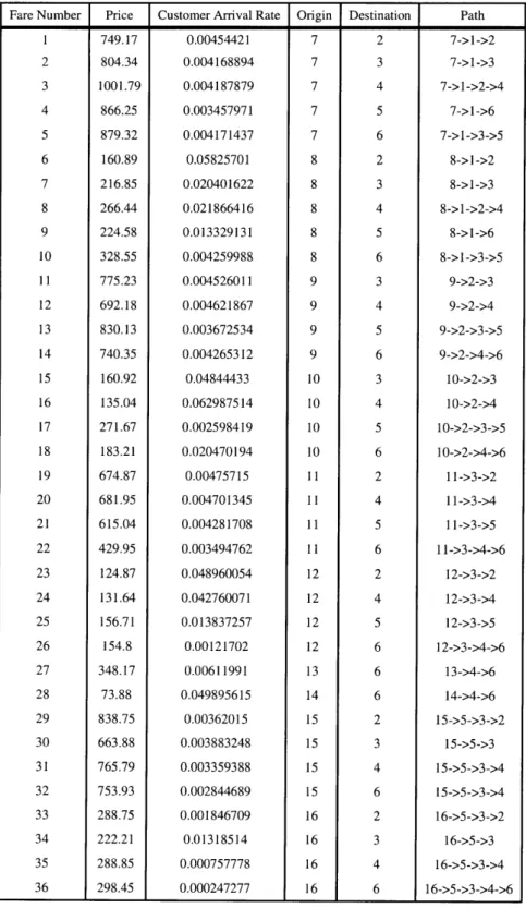
Parameter values for all fare products are shown in Table 1 along with the path (itinerary) used by each fare. The values shown in Table 3.1 are essentially arbitrary and were chosen merely to illustrate the performance of the heuristics; however, it is not hard to see that the revenue of the heuristics is affected only by the determin-istic fare prices and customer arrival rate. These prices and customer arrival rates are reasonable approximations of those found in actual airline applications as of the writing of Gallego and van Ryzin [6].

Fare Number Price Customer Arrival Rate Origin Destination Path 1 749.17 0.00454421 7 2 7->1->2 2 804.34 0.004168894 7 3 7->1->3 3 1001.79 0.004187879 7 4 7->1->2->4 4 866.25 0.003457971 7 5 7->1->6 5 879.32 0.004171437 7 6 7->1->3->5 6 160.89 0.05825701 8 2 8->1->2 7 216.85 0.020401622 8 3 8->1->3 8 266.44 0.021866416 8 4 8->1->2->4 9 224.58 0.013329131 8 5 8->1->6 10 328.55 0.004259988 8 6 8->1->3->5 11 775.23 0.004526011 9 3 9->2->3 12 692.18 0.004621867 9 4 9->2->4 13 830.13 0.003672534 9 5 9->2->3->5 14 740.35 0.004265312 9 6 9->2->4->6 15 160.92 0.04844433 10 3 10->2->3 16 135.04 0.062987514 10 4 10->2->4 17 271.67 0.002598419 10 5 10->2->3->5 18 183.21 0.020470194 10 6 10->2->4->6 19 674.87 0.00475715 11 2 11->3->2 20 681.95 0.004701345 11 4 11->3->4 21 615.04 0.004281708 11 5 11->3->5 22 429.95 0.003494762 11 6 11->3->4->6 23 124.87 0.048960054 12 2 12->3->2 24 131.64 0.042760071 12 4 12->3->4 25 156.71 0.013837257 12 5 12->3->5 26 154.8 0.00121702 12 6 12->3->4->6 27 348.17 0.00611991 13 6 13->4->6 28 73.88 0.049895615 14 6 14->4->6 29 838.75 0.00362015 15 2 15->5->3->2 30 663.88 0.003883248 15 3 15->5->3 31 765.79 0.003359388 15 4 15->5->3->4 32 753.93 0.002844689 15 6 15->5->3->4 33 288.75 0.001846709 16 2 16->5->3->2 34 222.21 0.01318514 16 3 16->5->3 35 288.85 0.000757778 16 4 16->5->3->4 36 298.45 0.000247277 16 6 16->5->3->4->6

Table 3.1: Price, customer arrival rate, origin-destination pair and path of each fare product in Example 1 network.

2 414' 4 """" L9 (150) L1 _L8 (150) (50) *. (50) (50).* L6 5 ... 1 .*(100) L4

OsWL

(100) (50) L ₁ 3 (100) (50) 11 + L5 (200) ₆

Figure 3-2: Example 2: A sixteen-node, product differentiated single hub airline network.

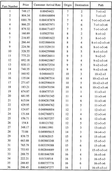
We also consider another exemplary product differentiated network with illegs and 36 fare products depicted in Figure 3-2. In this example, main hub is located at node 3, and two regional hubs are at node 1 and 5. Node 2 and 4 plays as connector and node 6 is arrival only destination. Parameter values for example 2 network is described in Table 3.2.

Fare Number Price Customer Arrival Rate Origin Destination Path 1 749.17 0.00454421 7 2 7->1->2 2 804.34 0.004168894 7 3 7->1->3 3 1001.79 0.004187879 7 4 7->]->2->3->4 4 866.25 0.003457971 7 6 7->1->3->6 5 879.32 0.004171437 7 5 7->1->3->5 6 160.89 0.05825701 8 2 8->1->2 7 216.85 0.020401622 8 3 8->1->3 8 266.44 0.021866416 8 4 8->1->2->3->4 9 224.58 0.013329131 8 6 8->]->3->6 10 328.55 0.004259988 8 5 8->1->3->5 11 775.23 0.004526011 9 3 9->2->3 12 692.18 0.004621867 9 4 9->2->3->4 13 830.13 0.003672534 9 5 9->2->3->5 14 740.35 0.004265312 9 6 9->2->3->6 15 160.92 0.04844433 10 3 10->2->3 16 135.04 0.062987514 10 4 10->2->3->4 17 271.67 0.002598419 10 5 10->2->3->5 18 183.21 0.020470194 10 6 10->2->3->6 19 674.87 0.00475715 11 1 11->3->1 20 681.95 0.004701345 11 4 11->3->4 21 615.04 0.004281708 11 6 11->3->6 22 429.95 0.003494762 11 5 11->3->5 23 124.87 0.048960054 12 1 12->3->1 24 131.64 0.042760071 12 4 12->3->4 25 156.71 0.013837257 12 6 12->3->6 26 154.8 0.00121702 12 5 12->3->5 27 348.17 0.00611991 13 3 13->4->3 28 73.88 0.049895615 14 3 14->4->3 29 838.75 0.00362015 15 4 15->5->4 30 663.88 0.003883248 15 3 15->5->3 31 765.79 0.003359388 15 6 15->5->6 32 753.93 0.002844689 15 1 15->5->3->1 33 288.75 0.001846709 16 4 16->5->4 34 222.21 0.01318514 16 3 16->5->3 35 288.85 0.000757778 16 6 16->5->6 36 298.45 0.000247277 16 1 16->5->3->1

Table 3.2: Price, customer arrival rate, O-D pair and path of each fare product in Example 2 network.

3.1

Clustering impact on revenue

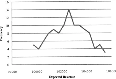
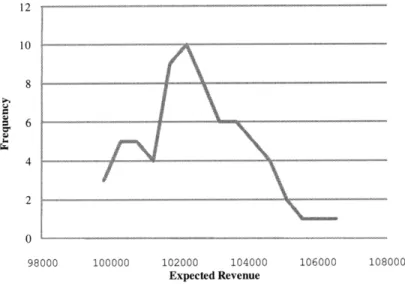
In order to understand significance of clustering on revenue, we have simulated 120 times on Example 1 network, by clustering random pairs of legs together. Also, simulated 70 times on Example 2 network by clustering random pairs of legs to-gether. Maximum revenue generated was 105475.5 and minimum was 99321.47 with standard deviation of 1510.612 as for Example 1 network. For Example 2 network, maximum revenue was 106534.6 and minimum was 98743.93 where standard devia-tion was 1613.006. The point of these experiments is to show the careful clustering impact. Where it can have on the performance of the resulting policy -upto 6.6% in the examples above. In all cases, the policy used is the greedy policy with respect to the approximation

E

J*. The middle 90% of revenue generated is within 101000 to

C

105000 where distribution is centered at 102800 as depicted in Figure 3-3. Histogram

on both cases shows that it is median centered distribution.

16 14 12 10 8 6 4

A

98000 100000 102000 104000 106000 Expected Revenue

Figure 3-3: Histogram of revenue for Example 1 network.

---10

8 6 4 2 0 98000 100000 102000 104000 106000 108000 Expected Revenue

Figure 3-4: Histogram of revenue for Example 2 network.

3.2

Heuristics on clustering

Although price improvement opportunity can be more than 6% by finding the right clustering, it can take very long time to find the optimal clustering. For example, in order to find best two leg clustering of 11 leg network, it requires 1247400 (approx. 1.2million) number of simulation to search the best clustering. We consider several generic heuristics to find clustering that maximize the revenue.

3.2.1

Cluster legs that shares the most number of fares

The decomposition approximation can apparently be improved by clustering legs that share the most number of fares in common. By clustering legs that share most number of fares in Example 1 network, revenue is 102992.7712 where average of random clustering is 102256 and minimum is 100826 for two leg clusters. This heuristic gave the revenue improvement of 2.11%. The clusters used in our experiment for Example

1 and Example 2 network are given in Table 3.3 and Table 3.4. In particular, we used

the following procedure to cluster legs.

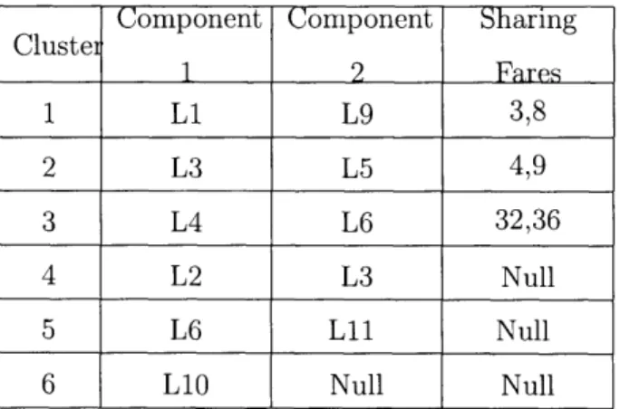
---Table 3.3: Cluster matches of Example 1 network for 3.2.1 heuristic.

Clustei Component Component Sharing

1 2 Fares 1 Li L9 3,8 2 L3 L5 4,9 3 L4 L6 32,36 4 L2 L3 Null 5 L6 11 Null

6 LIO Null Null

of Example 2 network for 3.2.1 heuristic.

1. Randomly select unclustered leg.

2. Select an unclustered leg that share as many fares as possible with the leg picked in step 1.

3. Put legs selected from step 1 and step 2 in the same cluster.

4. Go back to step 1 until there is no unclustered leg to select.

Component Component Sharing Cluster 1 2 Fares 1 Li L5 3,8 2 L4 L8 13,17 3 L7 L9 22,26,36 4 L2 L3 Null 5 L6 L11 33,29

6 LIO Null Null

3.2.2

Cluster legs that share high customer arrival rate fare

It is natural to expect that the quality of our approximation depends not only on the number of fares shared among legs in a cluster, but also, the arrival rate for these fares. So we can consider a heuristic that clusters legs that share high customer arrival rate fare. In particular we cluster legs as following:

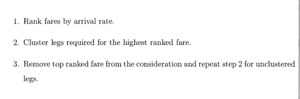
1. Rank fares by arrival rate.

2. Cluster legs required for the highest ranked fare.

3. Remove top ranked fare from the consideration and repeat step 2 for unclustered

legs.

The revenue was 103598 with price improvement of 2.71% for Example 1 network. For example, since fare 8 has the highest arrival rate among the fares that require multiple legs, leg 1 and 5 can be clustered together. The clustering used are given in the table below.

of Example 1 network for 3.2.2 heuristic. Component Component Cluster 1 2 1 LI L5 2 L4 L7 3 L6 L9 4 L2 L8 5 L3 L11 6 L1O Null

Table 3.6: Cluster matches of Example 2 network for 3.2.2 heuristic.

3.2.3

Cluster legs that share high priced fare

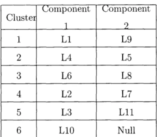
We can also cluster the legs based on the price rank of the fares. It generated revenue of 102960 with price improvement of 2.08%. In our example network, fare 3 has the highest price that for this heuristic we can cluster leg 1 and 5 together. Next expensive fare is fare 5 which demands leg 2 and 11. So we can cluster leg 2 and 11 into one cluster. The procedure used exactly as in section 3.2.2, with the exception that fares were ranked by fare prices.

Component

Component

Cluster 1 2 1 Li L5 2 L2 L11 3 L6 L8 4 L4 L7 5 L3 L9 6 L10 Null

Table 3.7: Cluster matches of Example I network for 3.2.3 heuristic. Component Component Cluster 12 1 Li L9 2 L4 L5 3 L6 L8 4 L2 L7 5 L3 L11 6 LIO Null

Component Component Cluster 1 LI L2 2 L4 L7 3 L3 L9 4 L5 L8 5 L6 L11 6 LIO Null

Table 3.8: Cluster matches of Example 2 network for 3.2.3 heuristic.

3.3

Local interchange heuristic

We can attempt to improve upon the clusterings produced by any of the aforemen-tioned heuristics by employing the following procedure.

With this scheme, we have ran 10 simulations with local interchange heuristic on both Example 1 and Example 2 networks. For Example network 1, this generated

1. Start with a random clustering (or a clustering produced from one of the

pre-vious heuristics).

2. Consider an arbitrary pair of clusters; say (i,

j)

and (k, 1).

3. Consider all swaps of legs between the two chosen clusters, (i, k) and

(j,

1), or (i, l) and (j, k).

4. Choose the swap that maximize the simulated revenue.

5. Go back to step 2.

revenue that is higher than other generic heuristics with average revenue of 104965.256 and maximum 105780.4. In the best case, it improved revenue by 4.84% by swapping max 40 times for Example 1 network. Since its local heuristic, it generates different revenue depending on the starting sequence of clusters.

110000 100000 90000 80000 70000 60000 50000

1

2

131415

6 7 8 9 10 ce0eExpectedRevenue 104645 014622 105301105731 104053 104936 105779 104457 105391104737 j@NumberofSwaps

J

8 25 31 21 16 32 40 23 17 22

Figure 3-5: Expected revenue and number of swaps generated by local interchange heuristic clustering in Example 1 network.

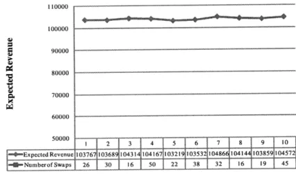
110000 100000 90000 80000 60000 70000 50000 ExpetedRevenue * j=Nmerofwps 2 3 4 5 6 7 8 9 * 103767 103689 04314 104167 03219 0353 104866104144 1038591104572 26 30 16 50 22 38 32 16 19 45

Figure 3-6: Expected revenue and number of swaps generated by local interchange heuristic clustering in Example 2 network.

inter-change heuristic to improve return revenue. With generic heuristic from section 3.2.2 as starting point, clustering with local interchange heuristic returned 107276.4 as rev-enue. This benchmark gave the best performance with improving revenue by 6.3%.

120000 110000 100000 90000 80000 70000 60000 50000 Expected Revenue Numberof waps 2 3 105732 107276.4 105301.1766 18 25 31

Figure 3-7: Revenue generated by clustering with local interchange heuristic + generic heuristic on Example 1. 120000 110000 100000 90000 80000 70000 60000 50000 40000 30000 20000₀ - - 2----3-flExpectedfRevenue 105358.6556 05747.622 105447.6947 26 30 16

Figure 3-8: Revenue generated heuristic on Example 2.

Chapter 4

Risk-Averse Model

4.1

The concept of risk-aversion

Decision makers might differ in their attitude towards risk. Within the theory of expected utility, different attitudes towards risk can be expressed by the shape of the utility function. An expected utility maximizing decision-maker with utility func-tion u is called risk-averse if one prefers the expected outcome of a non-degenerate lottery to the lottery itself. Representing a lottery by the random variable W with expectation E[W], this is equivalent to

(4.1) u (E[WJ) > E[u(W)]

for all lotteries W. Jensen's inequality yields that a decision-maker with utility func-tion u is risk-averse if and only if the utility function u is concave. In case of equality in (4.1), decision-maker's attitude is called risk-neutral. This holds for linear utility functions. Given the reverse inequality, the decision maker is risk-loving, which cor-responds to a convex utility function.

Now suppose the decision-maker had the choice between playing the lottery with random outcome W or receiving a certain amount of money w. The certainty equiv-alent of a lottery is the value of w that makes the decision-maker indifferent between

the two options. Thus, it fulfills

(4.2) E[u(W)] = u(w).

Consequently, the certainty equivalent can be defined as

(4.3) w = u1 (E[u(W)]).

If the utility function u is invertible. Choosing the lottery with highest expected

utility corresponds to choosing the lottery with highest certainty equivalent.

If we assume that the decision-maker is risk-averse, he prefers the expected

out-come of a lottery to playing the lottery. In other words,

(4.4) u(E[W]) > E[u(W)] = u(w),

using (4.1). Consequently, w < E[W] owing to the assumed monotonicity of u.

4.2

Single leg risk-averse model

Extending from general model described in Chapter 2, we now consider a model where decision maker is in risk-averse attitude. In risk-averse model, objective changes from maximizing revenue to maximizing utility. Utility can be described from utility function u(w) that is nonlinear and takes accumulated wealth, w, as variable. In order to solve this sequential decision problem that aim at maximizing expected utility can be solved by a Markov decision process if the state space is enlarged by another variable w, the accumulated wealth up to the current period.

For single leg problem we define the state-space1 S =

{x

:

E

Z+, x < xo} x

{w

w E Z+, w ' wo} x {t : t E Z+, t < T} and encoding the products offered for sale

at time t by a vector in a where a E {0, 1}F = A. State transition function, S is 'We assume prices are integer valued.

mapping S x {0, 1}F S4 S. It can be described as below transition function. (4.5) (X - 1, w + Pi, t + 1), w.p. Aia1I{xo} S a, if 0 < t < T

(X, w, t + 1), w.p.

1

-(F AfafI{f>o)

(X, w, t) , otherwise

A control policy 7r is mapping function 7r : S 1+ {0, 1}F. Let I be the set of all such policies. Let R(x, w, t, a) be a random variable representing revenue generated

by the airline when fare products a E A are offered for sale, and we have x seats left.

Then,

T-1

(4.6)

J'(xo, wo, 0) = E

R(Xt, 7r(Xt)) Xo =o

.t=oI

where Xt = S(Xt_1, r(Xt_1)). Then let maxrnJ'(x, w, t) J*(x, w, t), denote the

expected revenue under the optimal policy 7r* upon starting in state (x, w, t) E S.

J* and r* can be computed via dynamic programming. We can define the dynamic programming operator T according to

FF (T J) (x, w, t) = 1 - E Af J(z, w, t + 1)

f=1

(4-7) F +

E

Af max (If.,>o (J(x - 1, w + Pf, t + 1), J(x, w, t + 1)) f=1 af + (1 - I(>oj) J(x, w, t + 1))

We define (TJ)(x, w, T-1) = u(w) for the (T -1)-th horizon. J* can then be idenified as the unique solution to the fixed point equation TJ = J. 7r* is then the policy that achieves the maximum utility in (4.7). So, r* = 0 iff J(x - 1, w + Pf, t + 1) <

4.3

Single leg numerical example

We next examine numerical example of our model. In this example, there is 50 seats available for a single leg route, where finite time horizon of 1000 steps. This route starts from origin A and ends at destination B with only one leg as depicted in Figure 4-1. There are two fare products offered in this route where arrival process is un-correlated to each other. Fare 1 has time homogeneous arrival with customer arrival rate of 0.1. Fare 2 also has constant customer arrival rate of 0.05 where customer only arrives after 500th time step. Fare 1 is priced at 100 and Fare 2 is priced at 200.

(50)

Figure 4-1: Network with single leg, L1, with 50 seats available.

With given setting, we can maximize expected utility by computing via dynamic programming model from section 4.2. u(w) = w(1-k) is used for risk-averse utility

function, where k is risk-aversion parameter. So, more risk-averse it is, higher the k value.

With different risk-aversion k values, we computed value functions via dynamic programming and ran simulation from stored value function to calculate expected revenues and standard deviations of these revenues. Simulation results shows that As risk-aversion parameter k increases, standard deviation decreases.

Risk Aversion Expected Standard

Confidence

Interval

Parameter k

Revenue

Deviation

Range

Range

Minimum

Maximum

0

7432.54

483.1499

7431.012146

7434.067854

0.9

7421.08

480.1393

7419.561666

7422.598334

1-10-9

6787.4

354.5888

6786.278692

6788.521308

1-10'

5

5088.66

148.4918

5088.190428

5089.129572

Table 4.1: Expected revenue, standard deviation, and confidence interval of simula-tion result.

8000 7000 , 6000 S5000 .~4000 3000 rl 2000 1000 0 k k=0.9 k=1-10 0 100 200 300 400 500 600 Standard Deviation

Figure 4-2: Expected revenue vs. standard deviation over different k value. As shown in Figure 4-2, as risk-averse parameter k increases, standard deviation decrease and also expected revenue decrease. As decision-maker's attitude becomes more risk-averse, seats are sold more to Fare 1 in earlier stage in time. However, as decision-maker becomes less risk-averse, seats are kept unsold for longer period until higher priced Fare 2 customer arrives. If decision maker wait until Fare 2 customer to arrive, there is higher risk that he may not sell all seats by end of finite time horizon. However, by selling seats to Fare 2 customer as many as possible, he can gain higher wealth at the end. The more risk-averse decision maker's attitude is, less risk one

has to take and lower expected revenue and standard deviation. So, this simulation result coincide with decision maker's risk attitude.

4.4

Network risk-averse model

It is natural to extend single leg model into muli-leg network risk-averse model. In network risk-averse model, the airline company runs F fare products in L legged network at the same time. We define the matrix A = [AI,f], where Ai,1 E {0, 1}

depending on whether fare

f

consumes a seat on leg I or not. Each fare product is associated with a price P and requires seats on one or more legs. Initial capacity on each leg is given by a vector xo E Zt. Time is discrete. We assume a T period

horizon with at most one customer arrival in a single period.

Similar to clustering model in Chapter 2, we can approximate the optimal value function for network case by decomposing the network into individual legs instead of clusters. Then associated reward for each fare product on particular leg I is Pf a,f where fare coefficient a is defined as ai,f = 1,1 ' We define the state-space S' =

F Alf

1

{x : 1 E Z+,X1 < } x {w1 : W E R+,w > w1} x {t : t E Z+, t < T} and encoding the products offered for sale at time t by a vector in a where a E

{O,

1}F --.

For each leg, 1, state transition function, S' is mapping S' x A S1 -N S. It can be

described as below transition function. (4.8)

(X' - A1,1, W + Pa, 1, t + 1), w.p. Aia1IfX1>A, }

Sif 0 < t < T (Xz, w1, t + 1), w.p. 1- (F Afaf{X I}> ,)

f=1

(9i, wt, t) , otherwise

A control policy is a mapping 7r, : S 14 {0, 1}F. Let II, be the set of all such policies. Let R'(x', w', t, a) be a random variable representing revenue generated by the airline when fare products a E A are offered for sale, and we have x, seats left. Then,

~T-1

(4.9) J[" (x', w', 0) = EE R(X, 71 (X1)

|X1

= xi

t=0

where X = S'((X _ ), 7rl(X1t_ )). Then we let maxr, -nJ''(X, w , t) = J1*(X1, w ),

denote the expected revenue under the optimal policy 7r* upon starting in state

(Xi, w, t) E S.

programming operator T according to

(T JI)(x', w', t) = - Af J, (XI, w, t + 1)

f=1

F

(4.10) + E Af Max Ix>Al~} (Ji(x' - Al,f, w' + Pf a1 , I t + 1), Ji(iX, w1, t + 1))

f=1 af if

+ (I - I(;X1>Af} J (. I, w1, t + 1))

We define (TJi)(xi, wt, T - 1) = u(wl) for the (T - 1)-th horizon. J* can then be idenified as the unique solution to the fixed point equation TJ = J. Ir* is then the policy that achieves the maximum utility in (4.10). So, r* = 0 iff Ji(x' - Ai,1, wl +

Pf aij, t + 1) < J, (xi, w, t+ 1) and t < T.

L

Sum of these leg wise decomposed value function,

E

J,* (x', wl, t), is an upper-i=1

bound to optimal value function of the network, J* (x, w, t).

4.5

Network model numerical example

In this section, we examine numerical example of network risk-averse model. Example network is depicted in Figure 4-3, and corresponding seat capacity and leg numbers are listed in Table 4.2. There are 18 fare products offered in this 10 leg network within 1000 time steps. All corresponding fare product's price, customer arrival rate and path are listed in Table 4.3. All fare products' customer arrival rate is time homogeneous, where high priced fare has low customer arrival rate and low priced fare has high customer arrival rate.

Figure 4-3: Example network for network risk-averse with leg number and seat capacity in paranthesis.

model. Each legs are notated

Leg number Start Node End Node Seat Capacity

LI 1 2 150 L2 1 3 50 L3 1 6 50 L4 2 3 100 L5 2 4 200 L6 3 2 100 L7 3 4 100 L8 5 3 50 L9 4 6 150 L10 3 5 50

Table 4.2: Expected revenue, standard deviation, and tion result.

simula-Table 4.3: Expected tion result.

revenue, standard deviation, and confidence interval of

simula-With Given setting, we can maximize expected utility by computing via dynamic programming model from section 4.4. Similar to single leg risk-averse model, we used

u(w) = w(1-k) as our risk-averse utility function, where k is risk-aversion parameter.

Although the backward induction procedure for the finite horizon expected utility objectives only considers the relevant wealth levels at the different decision time steps, so the complexity of maintaining all wealth levels is too high. Suppose that the num-ber of distinct non-zero fare price is n. In the worst case, the numnum-ber of wealth levels to be considered at time step t is

('

"), which is the number of combinations for

se-lecting t items from t+n classes allowing repetition. Thus, complexity of representing different wealth level to perform backward induction is (t") = n = O(t"), an

n-th order polynomial in t, and thus computationally impractical if n is big. There-fore, some kind of approximation is needed and we uniformly discretized wealth levels

by increments of 50. We have chosen 50 as our wealth level increament, since 73.88

is the lowest price among fare products in our case.

Also, we discretized the wealth level into 1000 different wealth levels with increa-Fare Number Price Customer Arrival Rate Origin Destination Path

1 160.89 0.068485844 1 2 1->2 2 216.85 0.023983763 1 3 1->3 3 266.44 0.025705747 1 4 1->2->4 4 224.58 0.015669475 1 5 1->6 5 328.55 0.005007962 1 6 1->3->5 6 160.92 0.056950242 2 3 2->3 7 135.04 0.074046935 2 4 2->4 8 271.67 0.003054652 2 5 2->3->5 9 183.21 0.024064375 2 6 2->4->6 10 124.87 0.057556518 3 2 3->2 11 131.64 0.050267934 3 4 3->4 12 156.71 0.016266819 3 5 3->5 13 154.8 0.001430706 3 6 3->4->6 14 73.88 0.058656346 4 6 4->6 15 288.75 0.002170956 5 2 5->3->2 16 222.21 0.015500202 5 3 5->3 17 288.85 0.000890830 5 4 5->3->4 18 298.45 0.000290694 5 6 5->3->4->6