Charge transport and breakdown physics in liquid/solid insulation systems

(1)

Charge Transport and Breakdown Physics in

Liquid/Solid Insulation Systems

by

Jouya Jadidian

B.Sc., University of Tehran (2006)

M.Sc., University of Tehran (2008)

Submitted to the Department of Electrical Engineering and Computer Science in partial

fulfillment of the requirements for the degree of

Doctor of Philosophy

at the

M

ASSACHUSETTS

I

NSTITUTE OF

T

ECHNOLOGY

June 2013

© Massachusetts Institute of Technology, MMXIII. All rights reserved.

Author__________________________________________________________________

Department of Electrical Engineering and Computer Science

May 20, 2013

Certified by______________________________________________________________

Markus Zahn

Thomas and Gerd Perkins Professor of Electrical Engineering

Thesis Supervisor

Accepted by_____________________________________________________________

Leslie A. Kolodziejski

Chairman, Department Committee on Graduate Students

(2)

(3)

!

- 3 -

Charge Transport and Breakdown Physics in

Liquid/Solid Insulation Systems

by Jouya Jadidian

Submitted to the Department of Electrical Engineering and Computer Science in partial fulfillment of the requirements for the degree of!

Doctor of Philosophy

Liquid dielectrics provide superior electrical breakdown strength and heat transfer capability, especially when used in combination with liquid-immersed solid dielectrics. Over the past half-century, there has been extensive research characterizing “streamers” in order to prevent them, as they are the main origins of electrical breakdown in liquid dielectrics. Streamers are conductive structures that form in regions of liquid dielectrics that are over-stressed by intense electric fields. Streamers can transform to surface flashovers when they reach any liquid-immersed solid insulation. Surface flashovers usually propagate faster and further than streamers in similar electric field intensity. Charge generation and transport is crucially important in liquid dielectric breakdown, since without the presence of the electric charge and its ability to migrate in the liquid dielectric volume and on the interface of liquid/solid dielectrics, streamers and surface flashovers are unable to develop.

In this thesis, we develop a finite element method transport model in one, two and three-dimensional geometries to help understand the complicated dynamics of electric charge transport and streamer breakdown in liquid dielectrics. This electrohydrodynamic model clarifies many of the mechanisms behind streamer/surface flashover formation, propagation and branching in typical liquid/solid dielectric composite systems. Several key mechanisms have been identified and added to the transport model of streamers, such as effects of electric field intensity on the ionization potential of liquid dielectric molecules and electron velocity saturation, which make the modeling results more realistic. In addition to improving the understanding of electrical breakdown physics in liquid-based insulation systems, a significant effort is made throughout this thesis research to enhance the stability, convergence, speed and accuracy of the model, making it a convenient and reliable tool for designing high voltage components that contain pure liquid dielectrics, nanofluids and liquid immersed insulation systems. This model, for the first time, is able to treat any given electrode shape and gap distance as well as any applied voltage waveform with accurate results, which provides a convenient preliminary way to verify the performance of an insulation system in terms of breakdown voltage, time to breakdown, electric field intensity distribution and ionization level. The model precision is validated through experimental records, analytical solutions and alternative modeling approaches wherever available. Specifically, we verify our one-dimensional numerical results with exact analytical solutions, and our two and three-dimensional modeling results with experimental data found in the literature or provided by ABB Corporate Research, Sweden. The streamer initiation voltages, number of streamer branches, breakdown voltages and currents are in excellent agreement with the experimental data compared to the prior theoretical research on liquid breakdown physics. Identical results obtained using a finite volume method also confirm the correctness of the finite element approach used in this thesis. The presented model can be employed to search for novel configurations of liquid immersed insulation systems including nanofluids and liquid/solid composite systems.

Thesis Supervisor: Markus Zahn

(4)

A

CKNOWLEDGEMENT

I have really enjoyed my MIT life. I have had a unique advisor, Professor Markus Zahn, who has treated me like his own son. I am profoundly grateful to him for sharing his knowledge and experience with me, for his encouragement and friendship during the course of my PhD research. I have learned so many invaluable things from him beyond the scope of graduate studies.

I also appreciate insightful comments of my thesis committee members, Professors Jeffrey Lang and Luca Daniel, at the defense and at our committee and individual meetings, which helped me take one step back and look at the big picture of my thesis research.

I am truly indebted to members of the ABB Corporate Research team in Västerås, Sweden, with whom I worked closely on this project: Dr. Nils Lavesson, Dr. Ola Widlund and Dr. Karl Borg, who provided technical advice, constructive criticism and encouragement. I would like to acknowledge the ABB Corporation for the financial and technical support of this research.

I am thankful to my friends and colleagues at the Laboratory for Electromagnetic and Electronic Systems for many discussions and their company: Dr. Shahriar Khushrushahi, Dr. George Hwang, Mohammad Araghchini, Uzoma Orji, Samantha Gunter, Samuel Chang, Wei Li, Richard Zhang, Juan Antonio, Jiankang Wang, Wardah Inam and Seungbum Lim. My warm appreciation is due to Janet Fischer and Dimonika Bray and all other MIT administrative staff, who always had time for helping me out, no matter how busy they were.

The work that resulted in this thesis began long before I arrived at MIT. The preparation for my PhD studies has to be traced back to my several years at the High Voltage Laboratory of the University of Tehran. I particularly would like to thank my former advisors, Professors Hossein Mohseni, Kaveh Niayesh and Amir Abbas Shayegani and all my colleagues at this lab, many of whom are now spread around the world. I especially would like to pay tribute to a wonderful friend and an outstanding scholar, Jamal Shakeri, who regrettably succumbed to cancer.

This thesis is dedicated to my parents, Marzieh and Abbas, who have always been concerned about my education. They gave me a rare name, a pure Persian word, which means a person who is ravenous to search out the causes of things: a researcher. As far back as I can remember, I have marveled at their selection: my name is the best gift I have ever received. They enthusiastically started teaching their four-year-old son reading and basic arithmetic, and now I sincerely believe whatever I have achieved is their accomplishment too. I also dedicate this thesis to my sister, Darya, who will soon be graduating with her undergraduate degree. Although it has been extremely difficult for all of us to be apart, they have embraced the separation with patience, only for the sake of my well-being and success.

I would like to express my sincere gratitude to my best friend and my wife, Sepideh, for her unconditional love and unwavering faith throughout the years of college and graduate school. She has been astonishingly strong and a steady source of confidence in difficulties we both have faced. I hope I will be able to return the favor, her technical comments and endless support, during the remainder of her PhD research at Tufts University.

(5)

!

- 5 -

Contents'

!

1. Introduction

29 1.1. Charge Generation and Transport in Liquid Dielectrics Leading to

Streamer Formation and Electrical Breakdown

30 1.2. Analysis and Modeling of Streamer Development in Liquid-Solid

Insulation Systems

31

1.2.1. One-Dimensional Analysts of Charge Transport in

Liquid-Solid Composite Dielectric Systems 33

1.2.2. Two-Dimensional Axisymmetric Modeling of Single Column

Streamer 33

1.2.3. Two-Dimensional Modeling of Breakdown Phenomena 34 1.2.4. Modeling of Surface Flashover on Liquid Immersed

Dielectrics 34

1.2.5. Fully Three-Dimensional Modeling of Streamer Branching 35

1.3. Main Contributions of Thesis

35 1.4. Thesis Outline

41 2. Pre-breakdown Mechanisms in Transformer Oil-Based Insulation

Systems

43 2.1. Streamer Initiation, Propagation and Branching in Transformer Oil

43 2.2. Interactions of Streamers Initiated in Transformer Oil with

Adjacent Solid and Gaseous Dielectrics

46 2.3. Effects of Additives on Breakdown in Transformer Oil

48

2.3.1. Different Hydrocarbon Molecules in Transformer oil 48 2.3.2. Nanoparticle Additives and Microparticle Contaminations 50

(6)

3. Numerical Simulation Problem Posing/Approach

53 3.1. Introduction to COMSOL Multiphysics Modeling of

Streamer/Surface Flashover

53 3.2. Problem Posing Elements

53

3.2.1. Simulation Geometry 54

3.2.2. Governing Equations 54

3.2.3. Boundary Conditions 55

3.2.4. Stabilization Techniques 55

3.2.5. Meshing Policies and Mesh Element Definitions 57

3.2.6. Numerical Solvers 59

4. One-dimensional Analysis and Modeling of Unipolar Charge

Transport in Liquid-Solid Composite Dielectric Systems

63 4.1. Migration of Unipolar Charge Carrier Transport between Cartesian,

Cylindrical and Spherical Electrodes in Liquid-Only Systems

64 4.2. Migration-Ohmic Analysis of Charge Transport in a Series

Liquid-Solid Dielectric System with Linear Charge Injection from a Planar

Electrode

64

4.2.1. Governing Equations and Linear Charge Injection 65

4.3. Migration-Ohmic Analysis of Space Charge Limited Injection and

Transport in a Series Liquid-Solid Dielectric System

73

4.3.1. Cartesian Electrode Geometry 73

4.3.2. Coaxial Cylindrical Electrode Geometry 77 4.3.3. Concentric Spherical Electrode Geometry 82

4.4. Comparison of Analytical Solutions and Modeling Results

87 4.5. Summary

91 5. Two-dimensional Electrohydrodynamic Modeling of Streamer

(7)

!

- 7 -

5.1. Electrode Geometries and Gap Distances

94 5.2. Governing Equations

95 5.3. Charge Carrier Characteristics

97

5.3.1 Ionization Mechanisms 97

5.3.2 Recombination of Charge Species 100 5.3.3 Electric Field Dependent Electron Mobility 102 5.3.4 Temperature Dependent Electron and Ion Mobilities 104

5.4. Boundary Conditions

104 5.5. Breakdown Stages in Liquid Dielectrics

105

5.5.1 Streamer Initiation: Effects of Applied Voltage Parameters 107 5.5.2 Streamer Initiation: Effects of Electrode Geometries 123 5.5.3 Streamer Acceleration due to Re-ignition from Needle

Electrode 126

5.5.4 Breakdown Completion: Effects of Gap Distance and

Electrode Geometries on Full Breakdown 131

5.6. Summary

138 6. Three-dimensional Electrohydrodynamic Modeling of Streamer

Development and Branching in Dielectric Liquids

139 6.1. Spatial Inhomogeneities: Stochastic Origins of Branching

139

6.1.1. Visible Macro- Inhomogeneities 140 6.1.2. Stochastic Micro-Inhomogeneities 140

6.2. Three-Dimensional Modeling of Streamer Initiation and

Branching

141 6.3. Numerical Implementation of Stochastic Inhomogeneities

144 6.4. Modeling Results: Streamer Stochastic Branching Driven by

Micro-Inhomogeneities

146

(8)

6.6. Summary

167 7. Surface Flashover Formation and Growth on Liquid Immersed

Dielectrics

169 7.1. Streamer Interaction with Perpendicular and Parallel Liquid

Immersed Dielectric Interfaces

170 7.2. Surface Flashover Development on a Parallel Liquid Immersed

Dielectric Interface

176

7.1.1 Liquid Immersed Dielectrics with Greater Permittivity than

the Liquid (Pressboard in transformer oil) 177

7.1.2 Liquid Immersed Dielectrics with about the Same Permittivity

as the Liquid (PTFE in transformer oil) 178

7.1.3 Liquid Immersed Dielectrics with Smaller Permittivity than

the Liquid (SF6 in transformer oil) 179

7.3. Surface Flashover Development on a Perpendicular Liquid

Immersed Dielectric Interface

181

7.3.1 Liquid Immersed Dielectrics with Greater Permittivity than

the Liquid (Pressboard in transformer oil) 183

7.3.2 Liquid Immersed Dielectrics with about the Same

Permittivity as the Liquid (PTFE in transformer oil) 185 7.3.3 Liquid Immersed Dielectrics with Smaller Permittivity than

the Liquid (SF6 in transformer oil) 185

7.4. Sanity Checks

190 7.5. Summary

196 8. Concluding Remarks and Suggestions for Future Work

199 8.1. Streamer Initiation

199 8.2. Streamer Propagation

200 8.3. Streamer Branching

200

(9)

!

- 9 -

8.5. Streamer Branching

202 8.6. Sanity Checks

203 8.7. Future Work

203 Appendices:

207 A1. Optimized Combination of Artificial Diffusion Stabilization

Techniques for Finite Element Modeling of Drift Dominated Transport

of Charge Carriers

207 A2. Optimal Mesh Element Density Distribution for Streamer

Development Finite Element Modeling

209 A3. Simple Illustration of the Physical Differences between Positive and

Negative Streamer Formation in Dielectric Liquids

217 A4. Implementation of Stochastic Inhomogeneities

218 A5. Other Numerical Simulation Methods for Streamer Development

Modeling

220

(10)

List'of'Figures'

!

1.1. Streamer velocity plotted versus applied voltage peak as modeling obtained in this thesis (red square symbols), modeling results of others (green symbols) and experimental data found in the literature (blue symbols) for different electrode gap distances. The gap distances are labeled on the respective curves.

Experimental data are taken from different references (! [2]

,

●[4], ✵[6],

★

[7],

"[18], ▲[60], and

✳

[106]). The green symbols show the modeling results

O’Sullican [23] (◄) and Hwang [25] (►). 36 1.2. Streamer velocity plotted versus applied voltage peak as modeling obtained in

this thesis (red square symbols), modeling results of others (green symbols) and experimental data found in the literature (blue symbols) for different electrode gap distances. The gap distances are labeled on the respective curves.

Experimental data are taken from different references (![2]

,

●[4],

✵

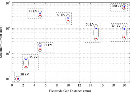
[6], "[18]). There is no prior modeling results on negative streamers. 37 1.3. Maximum pre-breakdown current plotted for different electrode gap distances.

Red square symbols show the modeling results of this thesis and blue symbols show the experimental data found in the literature. Each pair of data is labled with the associated applied voltage peak . Experimental data are taken from

different references (! [2]

,

!"[18], ►[60], and

✳

![106]).!! 38

1.4. Experimental data for a 6 mm gap (

#

), a 20 mm gap (▼), and a 50 mm gap (★), all obtained from [16]. Modeling results for a 6 mm gap distance (!). The solid curve, which is fitted to the modeling results, is Vi=10

2.2 _r

!, where rt is the

positive electrode tip radius in millimeters and the initiation voltage, Vi , is in

kilovolts. 38

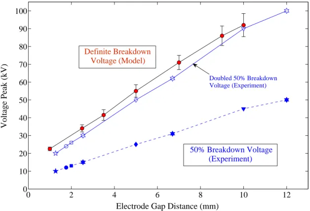
1.5. Modeling resutls (red symbols), obtained in this thesis, and experimental records (blue symbols), found in the literature, for breakdown voltages of different needle-sphere electrode gap distances. The model does not include statistical factors affecting the streamer formation and propagation. Therefore, the

calculated value for the definite breakdown voltage by the model, is rouphly two times greater than the 50% breakdown voltage which is determined after

numerous experiments. Experimental data are taken from different references

(![2]

,

!

●

[4],

✵

[6],

★

[7], "[18]).!! 39

1.6. Modeling resutls (red bars), obtained in this thesis, and experimental records (blue symbols), found in the literature, for number of active streamer branches emanating from a streamer node right after the branching, plotted versus the ratio of applied voltage peak over initiation voltage. Initiation voltage is mainly a function of the needle electrode tip radius. The model does not include statistical

(11)

!

- 11 -

factors affecting the streamer formation and propagation.Experimental data are taken from different references (![2]

,

●

[4],

★

[7], "[18], ▲[60], and✳ [106]). 40 2.1. (a): A positive streamer and (b): a negative streamer formed in the 5 mm gap

under different applied voltages (+26 kV and -52 kV). Filamentary structure of the positive streamer can be clearly distinguished from the thick and bushy shape of the negative streamer. The luminous plasma generated inside the channel formed by a negative streamer is also quite bulkier. The shock waves seen around the negative streamer supports the idea of formation of an appreciable gas

volume inside the negative streamer channel [8,18]. 44 2.2. (a) Time-integrated and (b-i) time resolved images of a streamer branching

during a positive/negative streamer conversion in 600 mbar artificial air. (j): A negative pulse of 35 kV is applied to the needle electrode (70 µm tip radius) for about 100 ns, followed by a positive voltage pulse for 150 ns, which creates positive streamers that run over the surface of the nearly spherical previously formed negative discharge. This is particularly interesting since it reveals that filamentary positive streamers and bubble shaped negative streamers can

interchange during a discharge [56]. 45

2.3. (Left) Single phase transformer windings covered by pressboard layers and (Right): Single phase high voltage transformer windings and bushing wound with pressboard layers ready for immersing in transformer oil. Courtesy of High

Voltage Laboratory, University of Tehran, used with permission. 47 2.4. Surface flashover development (a): within a polytetrafluoroethylene (PTFE) bore

[60] and (b,c): plate perpendicular to the streamer propagation direction [60,61]. 47 2.5. Time to breakdown (left) and average streamer velocity (right) versus applied

voltage peak provided by ABB Corporate Research in two different transformer oils for the needle-sphere geometry detailed in IEC Standard 60897 [66]. Positive and negative breakdown voltages of mineral oil types A and B are listed bellow:

Transformer Oil Positive Breakdown Voltage Negative Breakdown Voltage

Type A 105 kV 256 kV

Type B 126 kV 166 kV

49 2.6. Electric field lines for various times after a uniform z-directed electric field is

turned on at t=0 around a perfectly conducting spherical nanoparticle of radius R surrounded by transformer oil, and free electrons with uniform charge. The thick electric field lines separate field lines that terminate on the nanoparticle from field lines that go around the particle. The nanoparticles can assist and avoid breakdown by scavenging free electrons by intensifying and weakening the

electric field ahead of the positive and negative streamer heads, respectively. 51 3.1. COMSOL framework with different modules and interfaces. These modules can

be combined and cascaded to accomplish any complicated modeling task with

(12)

3.2. The plots compare the stabilized solution (dashed line) with the reference solution (solid line). a) unstabilized Galerkin formulation, b) stabilized formulation with isotropic diffusion, c) stabilized formulation with streamline anisotropic diffusion, d) stabilized formulation with SUPG diffusion, e)

stabilized formulation with SUPG diffusion and crosswind diffusion [71]. 58 4.1. Two-region, series planar, liquid-solid dielectric model excited by a

time-dependent current source, I(t), with Region I obeying a mobility (µ) conduction law and Region II obeying Ohmic conduction. 65

4.2. Nondimensionalized DC voltage V=Vεoilµ/ (σ a

2

)_{for various non-dimensional}

current densities J0=J / J0as a function of non-dimensionalized charge injection

coefficient A=Aa /εoil. 68

4.3. Space-time domain for the transient one-dimensional model of charge transport in the migration-Ohmic system for planar electrodes. In Region I, the

demarcation curve, xd(t), separates the initial condition problem (Sub-region I1) from the charge injection problem (Sub-region I2). The integration paths ζ1 and ζ2

in Region I and ξ1 in Region II, used to calculate terminal voltage are shown for

times less than the charge time of flight (td) starting at x=0, t=0 and ending at

x=a, t=td. Integration paths ζ3 and ξ2 in Region I /II are shown for times greater

than td. 70

4.4. Nondimensionalized voltage V=Vεoilµ/ (σ a

2

)between electrodes for various values

of nondimensionalized linear injection coefficient A=Aa /εoilas a function of

nondimensionalized time t=t µJ0/ (aεoil). 72

4.5. Two-region, series, oil-pressboard dielectric model for cylindrical electrodes excited by a step current source with Region I (Oil) for ri<r<rm obeying a mobility (µ) conduction law and Region II (Pressboard) for rm<r<ro obeying

Ohmic conduction. 78

4.6. Space-time domain for the transient one-dimensional model of charge transport in the migration-Ohmic system for coaxial cylindrical electrodes. In Region I, the demarcation curve, rd(t), separates the initial condition problem (Sub-region I1) from the charge injection problem (Sub-region I2). The integration paths ζ1 and ζ2

times less than the charge time of flight (td) starting at r=ri, t=0 and ending at

r=rm, t=td. Integration paths ζ3 and ξ2 in Region I /II are shown for times greater

than td. 81

4.7. Two-region, series, oil-pressboard dielectric model for spherical electrodes excited by a step current source with Region I (Oil) ri<r<rm obeying a mobility

(µ) conduction law and Region II (Pressboard) rm<r<r0 obeying Ohmic

(13)

!

- 13 -

4.8. Space-time domain for the transient one-dimensional model of charge transport in the migration-ohmic system for concentric spherical electrodes. In Region I, the demarcation curve separates the initial condition problem (Sub-region I1)

from the charge injection problem (Sub-region I2). The integration paths ζ1 and ζ2

times less than the charge time of flight (td) starting at r=ri, t=0 and ending at

r=rm, t=td. Integration paths to calculate terminal voltage ζ3 and ξ2 in Region I /II

are shown for times greater than td. 86

4.9. Non-dimensionalized voltage V=V / ( 2J_sa3

/ (9µεoil)+Jsa /σ)between electrodes

for the three electrode geometries treated in this chapter as a function of non-dimensionalized time t=t!_"µJ_s/ (σ a)#_$where all parameter values are defined in Table 4.3, and in particular a=0.0125 m is the oil region thickness in planar,

cylindrical and spherical geometries. 88

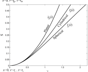
4.10. Non-dimensionalized steady state electric field E=Eε_oilµ/ (σa)_between

electrodes for different electrode geometries. Non-dimensionalized distance between positive electrode and interfacial surface is defined as S=S / (2a) which is

equal to x/(2a) for planar geometry, r/(2a)-0.5 for cylindrical geometry and r/(2a)-0.5 for spherical geometry. All parameter values are defined in Table 4.3, and in particular ri=ri=a=0.0125 m is the radius of the interior electrode in

cylindrical and spherical geometries respectively. 89 4.11. Non-dimensionalized space-time, trajectories for different electrode geometries

which show the demarcation curves in planar, cylindrical and spherical

geometries. Variable S is the demarcation trajectory x, r, and r given in equations (4.44), (4.62), and (4.82) for planar, cylindrical, and spherical geometries, respectively. Non-dimensionalized distance between the positive electrode and the interfacial surface is defined as S=S / (2a) which is equal to x/(2a) for planar

geometry, r/(2a)-0.5 for cylindrical geometry and r/(2a)-0.5 for spherical geometry as a function of non-dimensionalized time t=t µJs/ (aεoil) where all

parameter values are defined in Table 4.3, and in particular ri=ri=a=0.0125 m is the radius of the interior electrode in cylindrical and spherical geometries,

respectively. 89

4.12. Nondimensionalized volume charge density in the oil regions ρ=ρ µa / (εoilJs)

between electrodes for different electrode geometries in steady state. Nondimensionalized distance between the positive electrode and interfacial surface is defined as S=S / (2a) which is equal to x/(2a) for planar geometry,

r/(2a)-0.5 for cylindrical geometry and r/(2a)-0.5 for spherical geometry. 90

4.13. Nondimensionalized electric surface charge density at the oil/pressboard interface σs =σs/ (Jsεpb/σ − 2Jsεoila /µ)_{for planar, cylindrical and spherical}

(14)

5.1. Needle-sphere electrode chamber dimensions (left) and the actual electrode chamber in laboratory filled with transformer oil (right). This structure is used for experimental studies of streamers at ABB [55-57]. This exact geometry is also used for simulation purposes as described in IEC 60897 standard [66]. The electrodes are 25 mm apart and the radii of curvature of the needle and sphere

electrodes are 40 µm and 6.35 mm, respectively. 95 5.2. IEC 60060 lightning impulse voltage (non-dimensional, ) with rise-time

tr (10% to 90% of peak voltage) versus non-dimensional time,

generated with subtracting two exponential functions. 105 5.3. Electric field magnitude and lines (right side) and the net charge density and

equipotential lines (left side) for a positively applied lightning impulse voltage with 130 kV peak and 100 ns rise-time at t=155 ns. No discharges are observed for a 130 kV negatively applied impulse voltage. 108 5.4. Electric field magnitude and lines (right side) and the net charge density and

equipotential lines (left side) for a positively applied lightning impulse voltage

with 200 kV peak and 100 ns rise-time at t=100 ns. 109 5.5. Electric field magnitude and lines (right side) and the net charge density and

with 400 kV peak and 100 ns rise-time at t=100 ns. 110 5.6. Electric field magnitude and lines (right side) and the net charge density and

with 400 kV peak and 100 ns rise-time at t=200 ns. 111 5.7. Electric field magnitude and lines (right side) with the charge density generation

rate and equipotential lines (left side) for a negatively applied lightning impulse voltage with -400 kV peak and 1 ns rise-time at t=5 ns. 112 5.8. Electric field magnitude and lines (right side) with the charge density generation

rate and equipotential lines (left side) for a negatively applied lightning impulse voltage with -600 kV peak and 1 ns rise-time at t=5 ns. 113 5.9. Streamer head average distance from needle tip for positive and negative applied

voltages with different peak amplitudes. Positive streamer velocity tends to time increases, while a negative streamer decreases significantly after an initial bubble is formed around the needle. Error-bars show the range of results obtained by each of the artificial streamline diffusions (anisotropic, compensated streamline upwind Petrov-Galerkin and Galerkin least-square methods) to solve the charge continuity equations. The streamer velocity under +400 kV is roughly 2 times greater than +200 kV streamer velocity which is itself two times greater than +130 kV. Dissimilar rise-times for positive and negative streamers are shown to ease comparison between positive and negative streamers with velocities on the

same order. 116



V=V / V₀

(15)

!

- 15 -

5.10. Electric field magnitude and lines (right side) and the net charge density and equipotential lines (left side) for a positively applied lightning impulse voltage

with +200 kV peak and 50 ns rise-time at t=70 ns. 118 5.11. Electric field magnitude and lines (right side) and the net charge density and

with +200 kV peak and 10 ns rise-time at t=8.5 ns. 119 5.12. Electric field magnitude and lines (right side) and the net charge density and

with +200 kV peak and 2 ns rise-time at t=2 ns. 120 5.13. Volume charge densities and electric field distributions for different positively

applied voltage peak amplitudes and rise-times. The pictures are shown for the instant times that the streamer heads travel half a millimeter from the needle tip. Space charge densities are shown as filled contours from 0.5|ρmax| (the brightest color) to |ρmax| (the darkest color). Electric field contours are shown as black solid lines from 0.5|Emax| to |Emax|. The value of each contour is labeled on the curve as a fraction of |Emax|. The streamer head curvatures can be compared between streamers formed by (a): 130 kV with 1.2 µs rise-time: |Emax|=3.1×10

8

V/m , |ρmax|=4.25×10

3

C/m3; (b): 130 kV with 100 ns rise-time: |Emax|=2.9×10

8

V/m , |ρmax|=3.94×10

3

C/m3; (c): 200 kV with 1.2 µs rise-time: |Emax|=2.9×10

8

V/m , |ρmax|=3.12×10

3

C/m3; (d): 200 kV with 100 ns rise-time: |Emax|=2.8×10

8

V/m , |ρmax|=2.43×10

3

C/m3; (e): 400 kV with 1.2 µs rise-time: |Emax|=2.6×10

8

V/m , |ρmax|=1.54×10

3

C/m3; and (f): 400 kV with 100 ns rise-time |Emax|=2.4×10

8

V/m ,

|ρmax|=0.93×103 C/m3. 121

5.14. Electric field distributions and charge density generation rates for different negatively applied voltage peak amplitudes and rise-times. Space charge density generation rate, GM are shown as filled contours from 0.5|Gmax| (the brightest color) to |Gmax| (the darkest color). Electric field contours are shown as black solid lines from 0.5|Emax| to |Emax|. The value of each contour is labeled on the curve as a fraction of |Emax|. The approximate radius of an ionized bubble can be compared between different applied voltage peaks and rise-times: -250 kV with 1ns rise-time (upper right): |Emax|=1.01×108 V/m and |Gmax|=0.7×1011 Cm-3s-1; -400 kV with 1ns rise-time (middle right): |Emax|=1.42×108 V/m and

|Gmax|=1.2×1011 Cm-3s-1; -600 kV with 1ns rise-time (bottom right): |Emax|=1.75×10

8

V/m and |Gmax|=6.21×10

11

11

Cm-3s-1. 122

5.15. Experimental data for a 6 mm gap (

#

), a 20 mm gap (▼), and a 50 mm gap (★), all obtained from [16]. Modeling results for a 6 mm gap distance (!). The solid curve, which is fitted to the modeling results, is Vi=102.2 r!, where rt is the

positive electrode tip radius in millimeters and the initiation voltage, Vi , is in

(16)

5.16. A set of different positive needle electrode tip sizes with the same gap distance and applied voltage, which is slightly above the initiation voltage for all of the

positive electrode radii of curvature. 124

5.17. A set of different grounded tip sizes with the same gap distances and applied voltages. Ionization (high electric field) region is larger at sharper grounded

electrodes. 125

5.18. Electron velocity models and ionization potential (derived by Density Functional Theory) as functions of electric field intensity, ve=v0|E|/(|E|+E0). The numerical

values of parameters of the saturated electron velocity are labeled on the curves and ionization potential constants are set as Δ=1.36×10-18 J, γ=1.118×10-22

Jcm1/2V-1/2. Values v0= 41 km/s, E0=0.1 MV/cm is used in [2,3]. 126

5.19. Electron charge density and flux distributions obtained by the ordinary model with constant electron mobility (left panel) and the ESV model (right panel) under a similar applied voltage with 500 kV peak and 100 ns rise-time. Each panel shows two frames of the streamer, i.e., the stem of the streamer (which attaches to the needle electrode tip) and the streamer head. Both streamer heads are at the same distance from the needle tip, but at slightly different time instants (after 0.6 µs for the linear model with constant electron mobility and after 0.57

µs for the ESV model). 127

5.20. Charge carrier density (a), flux (b) and electric field distribution (c) obtained from the ESV model approximately 2 mm from the needle electrode tip while the streamer head is 5 mm from the needle tip under an applied voltage with 500 kV and 100 ns rise-time. Due to the electron velocity saturation, the electron and ion charge density do not quite cancel. Therefore, a secondary frontier of electric field is created inside the streamer column. In the case of E0=0.1 MV/cm, this

secondary frontier propagates slowly, however, for smaller E0, the secondary

frontier can propagates much faster and even collide with the main frontier

(streamer head front). 128

5.21. Electric field distributions in the range of 0.5|Emax| as the brightest color to |Emax|

as the darkest color for positively applied impulse voltages with 0.1µs rise-time and 400 kV peak amplitude. The values of |Emax| at z=0, z=2 mm and z=3 mm are

3.24 MV/cm, 3.46 MV/cm and 3.58 MV/cm (except at t=0.52 µs that is 4.27 MV/cm), respectively. The velocity of the streamer front is approximately

doubled after collision. 129

5.22. Normalized length of the streamers for different applied voltage amplitudes. Dashed lines show the results of the constant electron mobility model adapted from the reference[48] and the solid lines show the ESV model results. Streamers accelerate abruptly under impulse voltages with higher amplitudes than 400 kV in the ESV model. The sudden acceleration happens exactly when the main and secondary streamer fronts collide. Error-bars show the range of results obtained by each of the artificial streamline diffusions (anisotropic,

(17)

!

- 17 -

compensated streamline upwind Petrov-Galerkin and Galerkin least-square

methods) to solve the charge continuity equations. 130 5.23. Minimum applied voltage peak required for reigniting a positive streamer from

the needle electrode placed 25 mm from a grounded sphere electrode against saturation electric field, E0. For saturation fields above 0.651 MV/cm no

re-ignition is observed (applied voltage peaks up to 10 MV are examined). 131 5.24. Normalized length of the streamers for different electrode geometries and gap

distances at breakdown voltages. Breakdown voltage is the minimum impulse voltage amplitude at which the streamer is able to reach the ground electrode and consequently breakdown occurs. The streamer lengths are fitted with exponential and single term polynomial curves for needle-needle and needle-sphere

geometries, respectively. Streamers require higher impulse voltage amplitudes to reach the grounded needle electrodes. The streamer velocity clearly increases

when the streamer approaches the grounded electrode at z=d. 132 5.25. Streamer breakdown in needle-sphere (a, b, c, d) and needle-needle (e, f, g, h)

electrode gaps, 10 mm apart. Streamers always emanate from the positive needle and eventually hit the grounded electrode. Electric field distributions are shown in the range of 0.5|Emax|, as the brightest color to |Emax|, as the darkest color for

positively applied impulse voltages with 0.1µs rise-time and different peak amplitudes. The values of |Emax| (for 0.1<z<9.9 mm) and breakdown time are (a):

3.24 MV/cm, 1.092 µs; (b): 3.06 MV/cm, 0.564 µs; (c): 2.98 MV/cm, 0.328 µs; (d): 2.56 MV/cm, 0.212 µs; (e): 3.48 MV/cm, 0.244 µs; (f): 3.47 MV/cm, 0.377 µs; (g): 3.46 MV/cm, 0.648 µs; and (h): 3.48 MV/cm, 0.782 µs. The maximum electric field, |Emax|, within 0.1 mm of electrodes is about 30% less. The

trajectories of streamers are reasonably similar to Figure 5.25 and can be approximately scaled by the applied voltage amplitude (considering the time to

breakdown). 134

5.26. Grounded electrodes’ displacement and conduction currents, through needle-needle and needle-needle-sphere electrodes 10 mm apart at their own breakdown voltages, i.e., 112 kV and 92 kV, respectively. The displacement current rises abruptly just after application of an impulse voltage by the background electric field while conduction currents increase dramatically when the streamer hits the ground electrode at the times corresponding to z/d=1 in Figure 5.24 (for d=10 mm). The streamer charge influences displacement current indirectly, by changing the electric field distribution inside the gap. However, the effect of the streamer charge on the displacement current is not appreciable since the streamer engages a negligible portion of the electrode surface. An initial rise in the

conduction current of needle-needle geometry is due to the intense electric field near the grounded needle that causes an appreciable ionization leading to a limited conduction current (~100 mA) until the streamer reaches the grounded

needle. 135

5.27. Grounded electrodes’ total current (conduction plus displacement), through different gaps and geometries at their own breakdown voltages. The current rises dramatically when the streamer hits the ground electrode at the times

(18)

corresponding to z=d in Figure 5.24. Displacement current dominates the total current just after application of the impulse voltage. Semi-exponential attenuation of the displacement current suggests that the displacement current decay obeys the dielectric relaxation time dictated by the electrode geometry and dielectric properties. Both the initial magnitude and the decay rate of the displacement current toward the grounded needle electrode are smaller than the sphere electrode. This is consistent with their geometries since the area of the needle surface electrode is ~ 10 times smaller than the sphere electrode surface area. The conduction current dominates the total current as the streamer reaches the

grounded electrode that leads to breakdown (dramatic rise of current). 136 5.28. Predicted breakdown voltage for different gap distances. Error-bars show the

range of results obtained by each of the artificial streamline diffusions

(anisotropic, compensated streamline upwind Petrov-Galerkin and Galerkin least-square methods) to solve the charge continuity equations. 137 6.1. Typical view of positive streamer branching in a liquid dielectric, (a)

experimental image of a positive streamer initiated from a needle electrode [16] and, (b): 3-D modeling result of a corresponding case (iso-surface plot of the electric field distribution). The streamer structures are qualitatively similar in experiments and simulations. The fractal structure of the streamer tree in the experimental image makes it possible to compare the modeling result also with

other nodes of the tree including the one at the needle electrode tip. 142 6.2. Iso-surface plot of electric field distribution as modeling result of streamer is

compared with corresponding experimental image in the inset image. Definite breakdown voltage, UDBD, for the modeling geometry (gap length, d=25 mm, and the electrode tip radius, ri =40 µm) is equal to 95 kV. In the experimental data, the applied voltages are expressed in terms of streamer initiation voltage, Vi, and 50% breakdown voltage, UBD, which is the impulse peak at which the dielectric breaks down in half of the discharge tests:

Modeling (peak, rise time) Experiment (Photography method and applied voltage peak)

2.85 Vi (0.9 UDBD), 1 ns Streak image of streamer formed by 2.18 Vi (0.33 U50BD =327 kV) in a 150 mm

gap with ri = 1 mm (U50BD ≈ 970 kV) [13,15]

147 6.3. Iso-surface plot of electric field distribution as modeling result of streamer is

compared with corresponding experimental image in the inset image. Definite breakdown voltage, UDBD, for the modeling geometry (d=25 mm, ri=40 µm) is equal to 95 kV. In the experimental data, the applied voltages are expressed in terms of streamer initiation voltage, Vi, and 50% breakdown voltage, UBD, which is the impulse peak at which the dielectric breaks down in half of the discharge tests:

6 Vi (1.9 UDBD) , 100 ns Streak image of streamer formed by 4.88 Vi (1.57 U50BD =583 kV) in a 100 mm gap with ri=1 mm (U50BD ≈ 370 kV) [13,15]

(19)

!

- 19 -

breakdown voltage, UDBD, for the modeling geometry (d=25 mm, ri=40 µm) is equal to 95 kV. In the experimental data, the applied voltages are expressed in terms of streamer initiation voltage, Vi, and 50% breakdown voltage, UBD, which is the impulse peak at which the dielectric breaks down in half of the discharge tests:

7.66 Vi (2.42 UDBD), 10 ns Schlieren images of streamer formed by 7.25 Vi (100 kV=5.55 U50BD, 30 ns) in a 2.5 mm gap with ri=25 µm (U50BD ≈ 18 kV) [15,18]

8.66 Vi (2.74 UDBD), 100 ns Streak images of streamer formed by 8.2 Vi (0.8 U50BD =24 kV) in a 3 mm gap with ri=5 µm (U50BD ≈ 30 kV) [15,105].

9 Vi (2.84 UDBD), 10 ns Schlieren images of streamer formed by 2.77 Vi (47 KV= 1.88 U50BD, 20 ns) in a 5 mm gap with ri=25 µm (U50BD ≈ 25 kV) [15,18]

10 Vi (3.16 UDBD), 100 ns Schlieren images of streamer formed by 7.25 Vi (5.55 U50BD =100 kV, 300

ns) in a 2.5 mm gap with ri=25 µm (U50BD ≈ 18 kV) [15,18]

compared with corresponding experimental image in the inset image. Definite breakdown voltage, UDBD, for the modeling geometry (d=25 mm, ri=40 µm) is equal to 95 kV. In the experimental data, the applied voltages are expressed in terms of streamer initiation voltage, Vi, and 50% breakdown voltage, UBD, which

(20)

is the impulse peak at which the dielectric breaks down in half of the discharge tests:

10.66 Vi (3.37 UDBD), 100 ns Shadowgraphy images of streamer formed by 11.1Vi (5.55 U50BD=100 kV, 1.2µs) in a 2.5 mm gap with ri=30 µm (U50BD ≈ 14 kV) [2,15]

11.33 Vi (3.58 UDBD), 10 ns Streak images of streamer formed by 10.23Vi (1.14 U50BD =30 kV) in a 2

mm gap with ri=5 µm (U50BD ≈ 30 kV) [15,105].

12.6 Vi (4 UDBD), 10 ns Intensifier gate photographs of streamer formed by 13.2 Vi (0.9 U50BD =304 kV)

in a 200 mm gap with ri = 40 µm (U50BD ≈ 340 kV) [14,15]

15.2 (4.8 UDBD) 10 ns Intensifier gate photographs of streamer formed by 16Vi (0.87 U50BD =304 kV) in a

200 mm gap with ri = 3 µm (U50BD ≈ 350 kV) [14,15]

15.83 Vi (5 UDBD), 100 ns Shadowgraphy images of streamer formed by 14.44 Vi (9.28 U50BD = 130 kV, 1.2µs) in a 2.5 mm gap with ri=30 µm (U50BD ≈ 14 kV) [2,15]

(21)

!

- 21 -

6.13. Iso-surface plot of electric field distribution as modeling result of streamer is compared with corresponding experimental image in the inset image. Definite breakdown voltage, UDBD, for the modeling geometry (d=25 mm, ri=40 µm) is equal to 95 kV. In the experimental data, the applied voltages are expressed in terms of streamer initiation voltage, Vi, and 50% breakdown voltage, UBD, which is the impulse peak at which the dielectric breaks down in half of the discharge tests:

16.1 (5.1 UDBD), 10 ns Intensifier gate photographs of streamer formed by 18.62 Vi (1.38 U50BD =304 kV) in a 50 mm gap with ri = 3 µm (U50BD ≈ 220 kV) [14,15]

18.3 Vi (5.8 UDBD), 100 ns Schlieren images of streamer formed by 20.1 Vi (4.3 U50BD =28 kV, 1 µs) in a 1 mm gap with ri =5 µm (U50BD ≈ 6.5 kV) [3,18]

159 6.15. Symmetrical streamer branching due to symmetric initial electron disturbance

distribution (planes of symmetry are x=0 and y=0) showing that the numerical instabilities are minor enough to guarantee that the branching occurs due to physical inhomogeneities. The propagation direction of the main streamer column is in –z direction. The left panel shows iso-surface plots of the electric field generated by streamer branching from different view planes (xy, xz and xy

plane views). 161

6.16. Streamer head configuration debined based on distribution of volume charge density. Three characteristic lengths, ra, rb and d are defined based on the distribution of charge density magnitude (0.5ρmax to ρmax) to study the streamer head instability growth, which ultimately cause the branching. Numerical modeling shows that the chance of branching increases as the head curvature ratio α=ra/d increases. Our previous studies on the 2-D streamer model (Chapter 5) show that increasing either applied voltage peak or applied voltage rate of rise

would increase α. 162

6.17. Colors show the applied voltage rise-times: black (1 µs), blue (100 ns), purple (10 ns) and red (1 ns). Marker shapes indicate the applied voltage peaks: 130 kV (✳), 200 kV (

★

), 250 kV (●), 300 kV (▼), 350 kV (!), 400 kV ("), and 500 kV (✕). The points are obtained by taking average from ten different inhomogeneity distributions, but with the same inhomogeneity radius, maximum intensity and

density of 5 µm, 104 Cm-3 and 1011 m-3, respectively. 164

6.18.

Actual span of data of each normalized characteristic length indicated with error bars. The streamer characteristic lengths are measured from of 280 simulation

(22)

cases (10 individual simulations with different inhomogeneities in each case) modeled within the parameter boundaries of |GMp| < 1010 Cm-3s-1, |ρp| < 104 Cm-3,

Cp = 10

11

m-3, 1 µm < Rp < 10 µm. The values shown in Figure 18 are midpoints in each case. Colors show the applied voltage rise-times: black (1 µs), blue (100 ns), purple (10 ns) and red (1 ns). Marker shapes indicate the applied voltage peaks: 130 kV (

✳

), 200 kV (★), 250 kV (●), 300 kV (▼), 350 kV (!), 400 kV

("), and 500 kV (✕). 165

7.1. Efficiency (left) and damage percentage (right) of liquid immersed solid dielecric (spacer) verus, εi, the ratio of the liquid permittivity over the solid LID

permittivity, for different pressboard materials (different plotted symbols), as reprted in [63]. The dilecetric efficiency is maximum and the damage on the

immersed dielectric is minimum where the permittivities are equal, εi =1. 169 7.2. Perpendicular (left) and parallel (right) liquid immersed dielectric (LID)

configurations in 25 mm apart needle-sphere electrode geometries. Two bottom panels show closer views of the perpendicular (left) and parallel (right) immersed dielectrics just next to the needle electrodes. Streamers initiate from the positive needle electrode, elongate through the oil bulk and possibly settle on the LID surface as shown by arrows in the bottom panels. The distance of the

perpendicular interfacial surface from the needle electrode tip varies in the range of 1- 4 mm and the diamter of the paralel bore varies between 100-400 µm. 172 7.3. Streamer/surface flashover initiation on the perpendicular [panels (a), (b)] and

parallel [panels (c), (d)] LID interfaces. The streamer formed in oil emanates from a needle under an impulse voltage with 400 kV peak and 0.1 µs rise-time hits the SF6 surface [panels (a), (c)] and the pressboard surfaces [panels (b), (d)].

7.4. Free volume charge in the oil region and its image charge in pressboard region close to the oil immersed barrier interface. The direction and magnitude of the force on the free volume charge caused by permittivity mismatch can be

calculated using the method of images [15]. 175 7.5. Intensity and direction difference across the interfacial surface of two dielectrics

due to the difference of permittivity. Left side of the figure shows the reason that the electric field magnitude is greater in pressboard region (in absence of surface charge density) and filed lines deflect inward when the pressboard permittivity is smaller than the oil. The right hand side shows the reason that opposite is true

(23)

!

- 23 -

7.6. Electric field distribution for flashovers expanding on the parallel LID surface under positive applied impulse voltage with (a): 200 kV peak and (b,c): 400 kV peak all with 0.1 µs rise-time. Panels (a) and (b) show surface flashover on PTFE and panel (c) shows surface flashover on a pressboard interface. At all panels, the flashover edge is about 1 mm from the needle tip. 176 7.7. Electric field magnitude distribution for parallel pressboard (PB) interface. The

streamers are formed by impulse voltages with 130 kV (first row), 200 kV (second row) and 400 kV (third row) peak amplitudes, all with 0.1 µs rise-time. Emin≈0 and Emax is given in each panel. 177

7.8. Electric field magnitude distribution for parallel PTFE interface. The streamers are formed by impulse voltages with 130 kV (first row), 200 kV (second row) and 400 kV (third row) peak amplitudes, all with 0.1 µs rise-time. Emin≈0 and

Emax is given in each panel. 178

7.9.

Electric field magnitude distribution for parallel SF6 interface. The streamers are

formed by impulse voltages with 130 kV (first row), 200 kV (second row) and 400 kV (third row) peak amplitudes, all with 0.1 µs rise-time. Emin≈0 and Emax is

given in each panel. 180

7.10.

Surface flashover edge trajectories on the parallel LID surface against time under applied impulse voltage with 130 kV, 200kV and 400 kV peaks and 0.1 µs rise-time. Purple markers and dashed curves show streamer head positions in oil-only system adapted from 2. Time t=0 corresponds to to the time that streamer reaches the parallel LID interface. Purple dotted curves are fitted polynomial expressions as 1.8×1012t1.9, 1.7×1011t1.7 and 2.3×109t1.38 [mm] for streamers formed by 130 kV, 200 kV and 400kV, respectively in oil-only systems which are valid for

t < 1 µs. 182

7.11.

Electric field distributions at the perpendicular interfacial LID surfaces 1 mm from the needle tip for applied voltages with 130 kV (top), 200 kV (middle) and 400 kV (bottom) peaks and 0.1 µs rise-time. Left panel shows the oil-pressboard interface with size scale of 5 µm for all three sections. Right panel shows oil-SF6

interface with size scale of 10 µm for all three sections. All surface flashover edges are 0.25 mm from the axis of symmetry. Again, it should be noted that the spatial scale of the left colmun is different from the right column. 183

7.12.

Electric field magnitude distribution for perpendicular pressboard interface. The streamers are formed by impulse voltages with 130 kV (first row), 200 kV (second row) and 400 kV (third row) peak amplitudes, all with 0.1 µs rise-time. Emin≈0 and Emax is given in each panel. 184

7.13.

Electric field magnitude distribution for perpendicular PTFE interface. The streamrs are formed by impulse voltages with 130 kV (first row), 200 kV (second row) and 400 kV (third row) peak amplitudes, all with 0.1 µs rise-time. Emin≈0

(24)

7.14.

Electric field magnitude distribution for perpendicular SF6 interface. The

streamers are formed by impulse voltages with 130 kV (first row), 200 kV (second row) and 400 kV (third row) peak amplitudes, all with 0.1 µs rise-time. Emin≈0 and Emax is given in each panel. 187

7.15.

Electric field magnitude distribution for perpendicular LID interfaces. The streamers are formed by impulse voltages with and 130 kV (first row), 200 kV (second row) and 400 kV (third row) peak amplitudes, all with 0.1 µs rise-time.

Emin≈0 and Emax is given in each panel. 187

7.16.

Surface flashover edge trajectories on the perpendicular LID surface against time for (a): pressboard with εr = 4.4 and (b): SF6 at five bar with εr =1.1 (b). “d” is the distance of the perpendicular interface from the needle tip. 189

7.17.

Normal component (z-direction) electric field distribution at the interfacial surface of oil/pressboard at z=250 µm distance from the needle having 200 kV peak and 100 ns rise-time at t=200 ns. The electric field strength is normalized to 1.2×107 V/m. The tangential component (r-direction) of electric field is continuous across the interface. Three perpendicular 5 µm segments have been chosen (using “cross-sectional plot parameters, line/extrusion”) to plot Ez, and ρ on. Yellow lines show electric field streamlines and white lines show

equipotential lines. 191

7.18.

Normal component (z-direction) electric field distribution on segment 1 shown in Fig. 7.16 at the oil/pressboard interfacial. The electric field strength is

normalized to 1.2×107 V/m. The distance is normalizd to 25 mm. 192

7.19.

Normal component (z-direction) electric field distribution on segment 2 shown in Fig. 7.16 at the oil/pressboard interfacial surface 250 µm far from the needle having 200 kV peak and 100 ns rise-time at t=200 ns. The electric field strength is normalized to 1.2×107 V/m. The distance is normalizd to 25 mm. 192

7.20.

Normal component (z-direction) electric field distribution on segment 3 shown in Fig. 7.16 at the oil/pressboard interfacial surface 250 µm far from the needle having 200 kV peak and 100 ns rise-time at t=200 ns. The electric field strength is normalized to 1.2×107 V/m. The distance is normalizd to 25 mm. 193

7.21. Space charge density on the segment 1 shown in Fig. 7.16 at the

oil/pressboard interfacial surface 250 µm from the needle having 200 kV

peak and 100 ns.

193

7.22.

Space charge density on the segment 2 shown in Fig. 7.16 at the oil/pressboard interfacial surface 250 µm from the needle having 200 kV peak and 100 ns. 194

(25)

!

- 25 -

7.23.

Space charge density on the segment 3 shown in Fig. 7.16 at the oil/pressboard interfacial surface 250 µm from the needle having 200 kV peak and 100 ns.

Space charge density is almost zero at this segment. 194

7.24.

Surface charge density at the oil/pressboard interfacial (shown in Fig. 7.16) surface 250 µm far from the needle having 200 kV peak and 100 ns at different time instants. The harsh oscillations observed in this plot is usual when we are using weak form boundary conditions and streamline artificial diffusion. These fluctuations are minimized using different arbitrary functions and weak

constraints. However, these oscillations are inevitable while streamline artificial

diffusion is applied. 195

7.25. Surface charge density at the oil/pressboard interfacial surface 250 µm from the needle having 200 kV peak and 100 ns rise-time at t=200 ns. Fitting is also provided using MATLAB parameters gaussian fit. Dotted data shows the envelops of the raw data and the solid lines show the fitted curve with similar

colors for each data. 196

8.1. Schematic view of the multiphase model of streamer propagation. There are three distinct physical phases: liquid, gas and plasma. For each phase one would have to solve different sets of equations, which also have to be interrelated. To reduce the number of elements and complexity of the model, one can assume the electric field to be uniformly distributed in the inter-electrode area. 204 A1. Different streamer propagation mechanisms under two different artificial

diffusions: electric field magnitude distribution solved by (left): upwind Petrov-Galerkin diffusion and (right): anisotropic diffusion. The applied voltage peak

magnitude to the positive needle is 200 kV and the rise-time is 100 ns. 208 A2. Off-axis branching in a streamer formed by a positive impulse with 200 kV and 1

ns rise-time still appears even with an extremely fine mesh around the needle

(colors and white lines depict electric field and equipotential lines, respectively). 210 A3. Off-axis branching in a positive streamer formed by a positive impulse with 200

kV and 1 ns rise-time disappears even with a fine mesh over a larger box around the needle (colors and white lines depict electric field and equipotential lines,

respectively). 210

A4. Electric field magnitude (color) and streamlines (white lines) for two different mesh element size distributions under a positively applied voltage (200 kV peak and 100 ns rise-time at time 85 ns). The two simulations are separately computed with the left side plot having a smooth fine mesh while the right side plot has a fine mesh within 40 µm and for the outer area beyond this box it has been freely

meshed. Both SD and CWD are applied. 211

A5. Different cases of element size transformation over space and spatial disturbances that they may produce, (a): critical disturbance over a big jump in element size; (b): negligible

(26)

disturbance over a small jump in element size; (c): a gradual rise in element size

minimizes the effect of numerical disturbances due to element size variation. 212

A6. Mesh refinement policy in the 3D model in the vicinity of the needle. Mesh refinement data is given in Table A1. 213

A7. Comparison of 3-D model result and 2-D model result for plasma mesh calibration for an applied impulse voltage with 200 kV peak and 100 ns rise-time after 80 ns (2-D model) and 84 ns (3-D model). The maximum electric fields are 3.54 MV/cm (2-D model) and 3.42 MV/cm (3-D model). The streamer heads are at almost equal distances from the

needle tip. 214

A8. Comparison of 3-D model result and 2-D model result for plasma mesh calibration for an applied impulse voltage with 200 kV peak and 100 ns rise-time after 80 ns (2-D model) and 84 ns (3-D model). The maximum electric fields are 3.54 MV/cm (2-D model) and 3.36 MV/cm (3-D model). The streamer heads are at almost equal distances from the

needle tip. 215

A9. An exemplary mesh selection process for a 2-D axisymmetric modeling. Similar processes have been employed for each cases presented in this thesis. 216 A10. Illustration of a negative streamer (left) and a positive streamer (right) formation

and propagation in a needle-plane geometry (which is similar to needle-sphere geometry). As can be seen the negative streamers initiate with wider front due to the lower mobility of the positive ions. Since positive ions are not as effective as electrons to shield the needle electrode electric field, the needle affects a larger space immediately after the voltage is applied to the electrode; therefore the initial ionized region becomes much bulkier than the positive streamers. This eventually leads to lower field enhancement ahead of negative streamers and decreases the average velocity compared to fast positive streamers which always keep their filamentary shape thanks to the highly mobile electrons constantly

forming at the ionization zone at the streamer head. 217 A11. The pillbox containing 12 inhomogeneities (red spheres) with 10 µm radius

adjacent to the needle electrode. The streamer branching results obtained with these inhomogeneities (an any other sizes above and below 5 µm radius) show less similarity to the experimental images than those modeling images taken from results generated with inhomogeneities with 5 µm radius, suggesting that in

practice, the effective inhomogeneities should have an average radius of 5 µm. 219 A12. The pillbox containing 12 inhomogeneities (red spheres) with 5 µm radius

adjacent to the needle electrode. The streamer branching results obtained with these inhomogeneities with 5 µm radius, show the maximum resemblance with experimental pictures suggesting that in practice, the effective inhomogeneities

(27)

!

- 27 -

List'of'Tables'

!

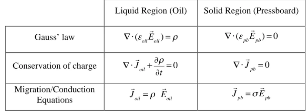
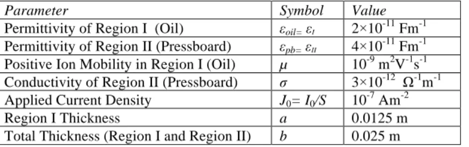
4.1. Governing Equations of Charge Transport in Liquid/Solid Insulation Systems 64 4.2. Parameters of dielectric Analysis with Linear Charge Injection Condition in

Cartesian Geometry 66

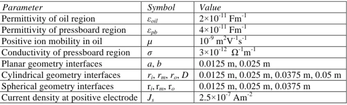
4.3. Numerical Parameter Values of dielectric Analysis with Space Charge Limited

Condition 87

5.1. Physical Parameters Used in the Streamer/Surface Flashover Model 99 7.1. Parameters of Investigated Transformer Oil-Immersed Dielectrics 171

A1. Mesh Data in Figure A6 214

(28)