Empirical photometric calibration of the Gaia red clump: Colours, effective temperature, and absolute magnitude

(1)

HAL Id: hal-02053736

https://hal.archives-ouvertes.fr/hal-02053736

Submitted on 1 Mar 2019

HAL is a multi-disciplinary open access

archive for the deposit and dissemination of

sci-entific research documents, whether they are

pub-lished or not. The documents may come from

teaching and research institutions in France or

abroad, or from public or private research centers.

L’archive ouverte pluridisciplinaire HAL, est

destinée au dépôt et à la diffusion de documents

scientifiques de niveau recherche, publiés ou non,

émanant des établissements d’enseignement et de

recherche français ou étrangers, des laboratoires

publics ou privés.

Empirical photometric calibration of the Gaia red clump:

Colours, effective temperature, and absolute magnitude

L. Ruiz-Dern, C. Babusiaux, Frédéric Arenou, C. Turon, R. Lallement

To cite this version:

L. Ruiz-Dern, C. Babusiaux, Frédéric Arenou, C. Turon, R. Lallement. Empirical photometric

cali-bration of the Gaia red clump: Colours, effective temperature, and absolute magnitude. Astronomy

and Astrophysics - A&A, EDP Sciences, 2018, 609, pp.A116. �10.1051/0004-6361/201731572�.

�hal-02053736�

(2)

DOI:10.1051/0004-6361/201731572 c ESO 2018

Astronomy

&

Astrophysics

Empirical photometric calibration of the Gaia red clump:

Colours, effective temperature, and absolute magnitude

?

L. Ruiz-Dern, C. Babusiaux, F. Arenou, C. Turon, and R. Lallement

GEPI, Observatoire de Paris, PSL Research University, CNRS UMR 8111, 5 place Jules Janssen, 92190 Meudon, France e-mail: laura.ruiz-dern@obspm.fr

Received 14 July 2017/ Accepted 16 October 2017

ABSTRACT

Context.GaiaData Release 1 allows the recalibration of standard candles such as the red clump stars. To use those stars, they first need to be accurately characterised. In particular, colours are needed to derive interstellar extinction. As no filter is available for the first Gaia data release and to avoid the atmosphere model mismatch, an empirical calibration is unavoidable.

Aims.The purpose of this work is to provide the first complete and robust photometric empirical calibration of the Gaia red clump stars of the solar neighbourhood through colour–colour, effective temperature–colour, and absolute magnitude–colour relations from the Gaia, Johnson, 2MASS, H

_ipparcos

, Tycho-2, APASS-SLOAN, and WISE photometric systems, and the APOGEE DR13 spec-troscopic temperatures.

Methods. We used a 3D extinction map to select low reddening red giants. To calibrate the colour–colour and the effective

temperature–colour relations, we developed a MCMC method that accounts for all variable uncertainties and selects the best model for each photometric relation. We estimated the red clump absolute magnitude through the mode of a kernel-based distribution function.

Results. We provide 20 colour versus G − Ks relations and the first Teff versus G − Ks calibration. We obtained the red clump

absolute magnitudes for 15 photometric bands with, in particular, MKs = (−1.606 ± 0.009) and MG = (0.495 ± 0.009) + (1.121 ±

0.128) (G − Ks− 2.1). We present a dereddened Gaia-TGAS HR diagram and use the calibrations to compare its red clump and its

red giant branch bump with Padova isochrones.

Key words. stars: fundamental parameters – stars: abundances – stars: atmospheres – dust, extinction

1. Introduction

Measuring distances with high accuracy is as difficult as fun-damental in astronomy. The most direct method for estimating astronomical distances is the trigonometric parallax. However, relative precisions of parallaxes decrease with distance. For dis-tant structures we need to use standard candles such as red clump (hereafter RC) stars.

Red clump stars are low mass core He-burning (CHeB) stars that are cooler than the instability strip. These stars appear as an overdensity in the colour–magnitude diagram (CMD) of popu-lations with ages older than ∼0.5−1 Gyr, covering the range of spectral types G8III – K2III with 4500 K . Teff . 5300 K.

In-deed, the RC represents the young and metal-rich counterpart of the horizontal branch (see Girardi 2016, for a review).

The RC is used as a standard candle for estimating astronomical distances due to its relatively small depen-dency of the luminosity on the stellar composition, colour and age in the solar neighbourhood (Paczynski & Stanek 1998; Stanek & Garnavich 1998; Udalski 2000; Alves 2000; Groenewegen 2008; Valentini & Munari 2010). As stated by Paczynski & Stanek (1998), any method to obtain distances to large-scale structures suffers mainly from four problems: the accuracy of the absolute magnitude determination of the stars used, interstellar extinction, distribution of the inner properties of these stars (mass, age and chemical composition), and the size

? _{Full Table}_A.1_{is only available at the CDS via anonymous ftp to}

cdsarc.u-strasbg.fr(130.79.128.5) or via

http://cdsarc.u-strasbg.fr/viz-bin/qcat?J/A+A/609/A116

of the sample. Whether the use of the RC may be considered par-ticularly different than other standard candles such as RR Lyrae or Cepheids, is precisely due to their large number. The larger the sample used, the lower the statistical error in distance calcu-lations. To efficiently use the RC as a standard candle, a good characterisation of the calibrating samples, here the solar neigh-bourhood, is needed, to which stellar population corrections can then be applied (see e.g.Girardi et al. 1998).

The first Gaia Data Release (GDR1) was delivered to the scientific community in September 2016 (Gaia Collaboration 2016). Although we will have new and more accurate astromet-ric and photometastromet-ric measurements for thousands of RC stars in future releases, this first catalogue includes the Tycho-Gaia As-trometric Solution (TGAS) subsample (Lindegren et al. 2016) that already has a significant set of accurate solar neighbourhood RC parallaxes; the systematic error is at the level of 0.3 mas, i.e. three times better than in the H

_ipparcos

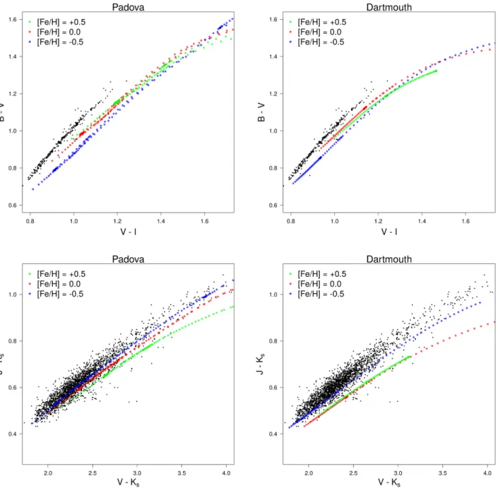
catalogue for 20 times more stars.

By comparing the observations with isochrones we can di-rectly constrain stellar parameters such as ages and metallici-ties. However, we found that at the level of red giant stars, at-mosphere models and observations do not fit: there is a gap between the models and observations no matter the photomet-ric bands nor the atmosphere models used. As an example, we show this issue in Fig.1 for the B − V versus V − I and J − Ksversus V − Kscolour–colour diagrams of some RC stars,

and for both Padova (Parsec 2.7) and Dartmouth isochrones, which use ATLAS and Phoenix atmosphere models, respec-tively. A more exhaustive work on the important effects on the

(3)

Fig. 1.B − Vvs. V − I and J − Ksvs. V − Kscolour–colour diagrams of RC stars (sample described in Sect.2). The median metallicity of the

sample is about −0.2. Padova Parsec 2.7 (left) and Dartmouth (right) isochrones with a median age of 2 Gyr are overplotted for three different metallicities: (green) [Fe/H] = +0.5, (red) [Fe/H] = 0.0, and (blue) [Fe/H] = −0.5. Only the red giant branch and the early assymptotic giant branch are shown.

choice of atmosphere models and other parameters may be found inAringer et al. (2016). We checked that a unique shift is not enough to correct this gap because the slope is also different. We also checked the influence of filter modelling. Nevertheless, it seems that it is most probably an issue of atmosphere models.

Therefore there are two aspects that led us to develop the purely empirical calibrations that we present in this work: first, the need for photometric calibrations totally independent of models; and second, the fact that there is no on-board Gaia calibrated filter profile (instrumental response) available for the GDR1, thus a colour–colour calibration was automatically needed. Jordi et al. (2010) already predicted some colour re-lationships based on theoretical spectra and the nominal Gaia passbands (calibrated before launch), but the effective filters ac-tually differ slightly (van Leeuwen et al. 2017). Therefore, there

is a special interest in using colour–colour empirical calibrations instead.

In this work we present the first metallicity-dependent empirical colour–colour (hereafter CC), effective temperature (Te_ff-colour and colour-Te_ff, hereafter Te_ffC and CTe_ff,

respec-tively) and absolute magnitude (MGand MK) calibrations for

so-lar neighbourhood RC stars using the Gaia G magnitude. The paper is organised as follows. In Sect.2we describe the sample selection, the adopted constraints and how the interstellar extinction has been handled. The method developed to calibrate all the CC and Teff relations is explained in Sect. 3. The

cali-brations obtained are presented in Sect.4. In Sect.5 we detail the RC absolute magnitude calibration. And finally in Sect.6we present the dereddened TGAS HR diagram and compare its RC to the Padova isochrones.

(4)

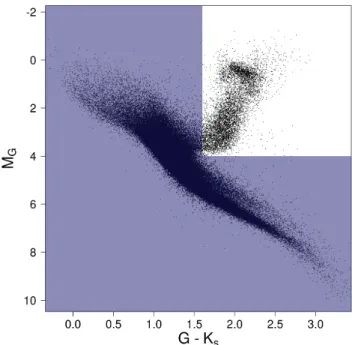
Fig. 2.TGAS HR diagram with parallax precision ≤10%, σG < 0.01,

EB − V < 0.015, and 2MASS JKs-bands high photometric quality (data

available in Table A.1, Appendix A). The non-shaded region corre-sponds to the selection of red giants with G − Ks> 1.6 and MG < 4.0.

2. Sample selection

Different samples were constructed using TGAS data for the colour–colour and the effective temperature calibrations. To en-sure their quality we considered the following constraints. 2.1. Interstellar extinction

One of the main issues with CC, TeffC and CTeff calibrations

for giants is the extinction handling. To select low extinction stars, we use here the most up-to-date 3D local extinction map ofLallement et al.(2014),Capitanio et al.(2017), together with the 2DSchlegel et al.(1998) map for stars for which the distance goes beyond the 3D map borders. We scaled theSchlegel et al. (1998) map values by 0.884 according toSchlafly & Finkbeiner (2011) and in agreement with theCapitanio et al.(2017) E(B − V) scale. We fixed a maximum threshold of 0.01 in E(B − V), i.e. 0.03 in A0, for a maximum distance corresponding to a parallax

$ − σ$. Such a selection of low extinction stars should lead to more robust results than a dereddening that would be dependent not only on an extinction map but also on an extinction law and could lead to either over or under correction of the extinction.

2.2. Selection of red giants

To select solar neighbourhood red giant stars we considered the following two criteria:

G − Ks> 1.6 (1) mG+ 5 + 5 log10 $ + 2.32 σ$ 1000 ! < 4.0. (2)

The factor 2.32 on the parallax error corresponds to the 99th percentile of the parallax probability density function. Figure2 shows the selected region on the HR diagram. The data used to construct this HR diagram is described in TableA.1. see Sect.6 for more details on the RC region of this diagram.

We extended the parallax criteria to cover the full red giant branch so that our calibrations have a larger interval of applica-bility than just the RC. We checked that this large magnitude interval did not have any significant impact on the calibra-tion. The fit is, on the contrary, very sensitive to red dwarf stars contaminants. Indeed the slope of giants and dwarfs in colour–colour distributions changes gradually as the stars are cooler (e.g Bessell & Brett 1988). A selection based on spec-troscopic surface gravity (2.5 < log g < 3.5) was tested and dis-carded because of the non-negligible percentage of giants/dwarfs misidentification in some surveys; for example, we found ∼2% misidentified RAVE stars when selecting those matching Ap-pendixAcriteria that are supposed to be inside the non-shaded region of Fig.2. The chosen parallax criteria allows us to guar-antee there is no contamination of dwarfs in our sample. 2.3. Photometric data

Our calibrations aim to cover all major visual and infrared bands. To achieve this we selected only those DR1 stars that have photo-metric information (with uncertainties) from the following cata-logues: GDR1, H

_ipparcos

, Tycho-2, 2MASS, APASS DR9, and WISE.

2.3.1. GDR1

We included stars with uncertainties lower than 0.01 mag in the G band. An error of 10 mmag was quadratically added to mitigate the impact of bright stars residual systematics; see Arenou et al.(2017),Evans et al.(2017).

2.3.2. HIPPARCOS

We selected stars with B, V, and Hp bands with uncertainties

lower than 0.03 mag. We did not include the I band because of the low number (∼12) of remaining stars when selecting those with V − I direct measurements in the Cousins system (field H42= A), with measurements in the Johnson system then con-verted to the Cousins system (field H42= C), and with measure-ments in the Kron-Eggen system then converted to the Cousins system (field H42 = E). For more details seePerryman et al. (1997), Vol. 1, Sect. 1.3, Appendix 5.

2.3.3. Tycho-2

We selected stars with BTand VTphotometric bands (Høg et al.

2000) with uncertainties lower than 0.03 mag. 2.3.4. 2MASS

We included those stars with J, H, and Ks photometry

(Cutri et al. 2003) from the cross-matched 2MASS-GDR1 cat-alogue (Marrese et al. 2017) with high photometric quality (i.e. flag q2M= A) and fromLaney et al.(2012). Only stars with un-certainties lower than 0.03 mag were chosen.

2.3.5. APASS DR9

We also considered stars with g, r, and i bands (Henden et al. 2016) cross-matched with Gaia at 200 precision, and only stars with standard deviations obtained from more than one obser-vation (ue = 0 flag in the APASS catalogue) and uncertainties

(5)

source with the largest number of photometric bands provided in APASS.

2.3.6. WISE

We selected stars with W1, W2, W3, and W4 photome-try (Wright et al. 2010) from the cross-matched WISE-GDR1 catalogue (Marrese et al. 2017) with uncertainties lower than 0.05 mag, high photometric quality (i.e. flag qph= A), low prob-ability of being true variables (i.e. flag var< 7), a source shape consistent with a point source (i.e. flag ex= 0) and showing no contamination from artefacts (i.e. flag ccf = 0). According to Cotten & Song(2016), for W2 we also removed stars brighter than 7 mag, because they are saturated.

2.4. Binarity and multiplicity

We removed all stars flagged as binaries and belonging to mul-tiple systems. To do so we took into account the specific flags in the H

_ipparcos

catalogue and the last updated information from the 9th Catalogue of Spectroscopic Binary Orbits (SB9, Pourbaix et al. 2004, 2009), the Tycho Double Star Catalogue (TDSC,Fabricius et al. 2002), and Simbad database (stars with flag “**”). We also considered only stars for which the proper motions from H

_ipparcos

are consistent with those of Tycho-2 (rejection p-value: 0.001). According to a specific test car-ried out in the framework of the Gaia data validation team (Arenou et al. 2017) most of the stars for which the proper mo-tions are not consistent between both catalogues are expected to be long period binaries not detected in H

_ipparcos

, and for which the longer time baseline of Tycho-2 could have provided a more accurate value.

2.5. Metallicity

We selected stars with metallicity information from various sources, since there were not enough stars when using just one reference. The expected effect of heterogeneity is that the dif-ferences between all the measurements will increase the dis-persion of the residuals and decrease the dependence of the calibrations with metallicity. Noting in brackets the percent-age of stars found and used in this work1, our established pri-ority order is:Morel et al. (2014) [0%],Thygesen et al.(2012) [0%], Bruntt et al. (2012) [0.04%], Maldonado & Villaver (2016) [0.6%], Alves et al. (2015) [1.4%], Jofré et al. (2015) [0.4%], Bensby et al. (2014) [0.4%], da Silva et al. (2015) [0.04%],Mortier et al.(2013) [0.04%],Adibekyan et al.(2012) [0.3%], APOGEE DR13 (SDSS Collaboration 2017) [9.9%], GALAH (Martell et al. 2017) [0.4%], Ramírez et al. (2014a) [0%], Ramírez et al. (2014b) [0%], Ramirez et al. (2013) [0.04%], Zieli´nski et al. (2012) [0.2%], Puzeras et al. (2010) [0.04%], Takeda et al. (2008) [0.08%], Valentini & Munari (2010) [0.6%], Saguner et al. (2011) [0%], RAVE DR5 (Kunder et al. 2017) [67.6%], LAMOST DR2 (Luo et al. 2016) [13.5%], AMBRE DR1 (De Pascale et al. 2014) [1.0%],Luck (2015) [0.7%], and PASTEL (Soubiran et al. 2016) [2.8%].

The final sample contained 2334 stars when considering the extinction, red giants selection, multiplicity, metallicity and the photometric constraints on the G and Ksbands. Subsamples were

then generated for each colour–colour relation depending on the other photometric bands used (see later in Table4the final sizes for every fit).

1 _{Some references used in our compilation could lead to no star in the}

final sample, i.e. 0% owing to the various quality cuts

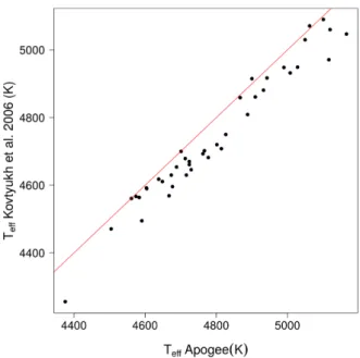
Fig. 3.Comparison of the spectroscopic effective temperatures of the 41 stars in common between APOGEE andKovtyukh et al.(2006).

2.6. Effective temperature

For the Te_ff calibrations the largest homogeneous sample

fill-ing all the above criteria is the 13th release (DR13) of the APOGEE survey (Holtzman et al. 2015;García Pérez et al. 2016;SDSS Collaboration 2017). To increase the sample size, we also included stars not in TGAS with APOGEE log g < 3.2, using therefore only the Schlegel et al. (1998) map to apply our low extinction criteria. The weighted mean of the parame-ters was computed for the duplicated sources. The cross-match with Gaia was carried out through the 2MASS cross-match (Marrese et al. 2017) with an angular distance <100_{. The final}

sample contained 530 stars.

The SDSS Collaboration discusses a systematic offset2 _of their spectroscopic effective temperatures from photometrically derived temperatures for metal-poor stars (by as much as 200– 300 K for stars at [Fe/H] ∼ −2). Consequently the authors pro-vided a correction as a function of metallicity. We decided not to apply their suggested correction as it is based on compari-son with photometric temperatures. We compared the APOGEE temperatures to the PASTEL temperatures and found metallicity correlations only for the most metal-poor stars ([Fe/H] < −1.5). We tested that our calibrations did not change significantly when we removed the most metal-poor stars from our sample.

For metal-rich stars, we compared 41 giant stars (within −0.4 < [Fe/H] < 0.2) fromKovtyukh et al.(2006) in common with APOGEE. These authors got a very good internal precision of 5–20 K (zero-point difference expected to be smaller than 50 K). As shown in Fig.3we find a difference of about 50 K with respect to APOGEE with no correlation with [Fe/H] and a dispersion in agreement with the precisions provided in both catalogues.

3. Calibration method

To derive accurate photometric relations, we implemented a Monte Carlo Markov Chain (MCMC) method, which allows us

2 _{http://www.sdss.org/dr13/irspec/parameters/}

(6)

to account and deal with the uncertainties of both the predictor and response variables in a robust way.

We provide all the calibrations with respect to the G − Ks

colour. Those photometric bands will be widely used thanks to the all-sky and high uniformity properties of the Gaia and 2MASS catalogues. Thus, in this work we provide the following calibrations:

Colour= f(G − Ks, [Fe/H])

ˆ

T = f(G − Ks, [Fe/H])

G − Ks= f( ˆT, [Fe/H]) (3)

where Colour includes all possible combinations of the pho-tometric bands considered in this work (Sect. 2.3), and ˆT = Teff/5040 is the normalised effective temperature.

3.1. Polynomial models

The general fitting formula adopted is

Y = a0+a1 X+a2 X2+a3[Fe/H]+a4[Fe/H]2+a5X[Fe/H] (4)

which is a second order polynomial3 where, following Eq. (3), Xis either the G − Ksor the normalised effective temperature ˆT,

Yis (for CC) a given colour to be calibrated or (for Teffrelations)

either G − Ks or ˆT, and aiare the coefficients to be estimated.

In order to provide the most accurate fit for each relation, the process (see Sect.3.3) penalises by the complex terms so that, in the end, seven different models may be tested for every relation (Model 7 being the more complex model) as follows:

Model 1: Y = a0+ a1X

Model 2: Y = a0+ a1X+ a2X2

Model 3: Y = a0+ a1X+ a3[Fe/H]

Model 4: Y = a0+ a1X+ a2X2+ a3[Fe/H]

Model 5: Y = a0+ a1X+ a3[Fe/H] + a4[Fe/H]2

Model 6: Y = a0+ a1X+ a2X2+ a3[Fe/H] + a4[Fe/H]2

Model 7: Y = a0+ a1X+ a2X2+ a3[Fe/H] + a4[Fe/H]2

+ a5 X[Fe/H].

Input uncertainties from all variables are taken into account in the model.

3.2. Monte Carlo Markov Chain

A MCMC was run for every model tested with 10 chains and 10 000 iterations for each. We used the runjags4 library from the R program language. An uninformative prior was set through a normal distribution with zero mean and standard deviation 10. Further, we also set an initial value for every coefficient. That is, we used the output coefficients obtained for each model through a multiple linear regression; this is a simpler method that does not take uncertainties into account, but allows to obtain approxi-mated values. The MCMC fit is run on the standardised variables to improve the efficiency of MCMC sampling (reducing the au-tocorrelation in the chains). Chain convergence is checked with the Gelman and Rubin convergence diagnostic.

3 _{Upper degrees were tested, but discarded by an analysis of variance}

test (ANOVA), meaning that simpler models were good enough to de-scribe the data

4 _{https://cran.r-project.org/web/packages/runjags/}

runjags.pdf

3.3. Best model selection: deviance information criterion The model selection was carried out through a process of penal-isation by the complex terms. To do so we took advantage of the deviance information criterion (DIC) (Plummer 2008), and we tested the models in pairs. A given complex model was com-pared to the next simpler model; for example, we removed the highest order interactions, starting with the cross-term X∗[Fe/H]. The method continuously determined the next pair of models to be compared, ran the MCMC for each and checked their DIC. When the DIC difference was significantly negative at 1σ (i.e. ∆DIC+σ∆DIC< 0) the complex model was kept, or else the next

pair was tested.

3.4. Outliers

Once the best model was determined, the method checked whether there were calibrated stars 3σ away from the model. If so, the furthest star was removed and the complete process was run again. Outliers were eliminated one by one to ensure that the further outlier was not causing a deviation in the model that led us to consider other stars as “false outliers”.

4. Calibration results

4.1. Colour–colour relations

Table1 gives the coefficients for each of the 20 colour versus G − Ks fit, together with the G − Ks and metallicity ranges of

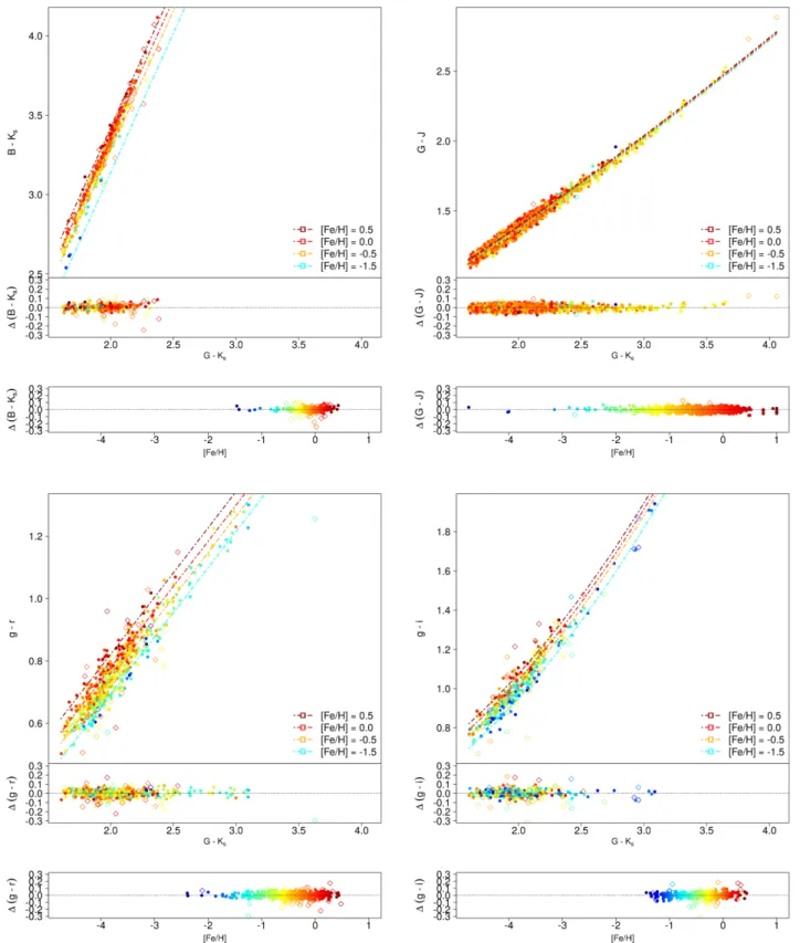
applicability, which are defined by the maximum and minimum values of each individual sample, along with the number (N) of stars used after the 3σ clipping, the percentage of outliers re-moved, and the final root mean square deviation (RMS). Figure4 shows the colour versus G − Ks relations obtained for 4 of the

20 colour indices with the residuals of the fit as a function of the colour itself and the metallicity. The scatter obtained in the residuals is very small (∼±0.03 globally).

4.2. Effective temperature calibration

Table2provides the coefficients of the fit for the ˆT versus G − Ks

and the G − Ksversus ˆTcalibrations. The colour, Te_ffand

metal-licity ranges of applicability are specified as well as the number (N) of stars used after the 3σ clipping, the percentage of outliers removed, and the final root mean square deviation.

Figure5 shows the ˆT versus G − Ksrelation obtained with

the residuals as a function of G − Ks colour index and

metal-licity. Since previous works in the literature use θ = 5040/Teff

instead of the ˆT considered here (e.g. Ramírez & Meléndez (2005),González Hernández & Bonifacio(2009) orHuang et al. (2015)), we also computed the calibration by using θ. We found both calibrations look similar except for the cool stars, for which we just have a few points. We may see how in this region the

ˆ

T relations at various metallicities cross each other in an unre-alistic way. This does not happen for the θ fit. However, after having statistically compared both the ˆT and θ calibrations, we chose to provide only the coefficients for ˆT versus G − Ks.

In-deed, DIC is significantly lower for the ˆT fit. The dispersion ob-tained on the Teff residuals is about 59 K, which is consistent

(7)

Table 1. Coefficients and range of applicability of colour versus G − Ksrelations, Y= a0+ a1(G − Ks)+ a2(G − Ks)2+ a3[Fe/H] + a4[Fe/H]2+

a5(G − Ks) [Fe/H].

Colour G − Ksrange [Fe/H] range a0 a1 a2 a3 a4 a5 RMS %outliers N B − G [1.6, 2.4] [−1.4, 0.4] 0.583 ± 0.180 −0.046 ± 0.187 0.215 ± 0.049 0.144 ± 0.006 − − 0.02 17.9 230 B − V [1.6, 2.4] [−1.4, 0.4] −0.094 ± 0.017 0.552 ± 0.009 − 0.129 ± 0.005 − − 0.02 10.4 251 B − J [1.6, 2.4] [−1.5, 0.4] −0.117 ± 0.041 1.432 ± 0.021 − 0.153 ± 0.011 − − 0.03 12.9 176 B − Ks [1.6, 2.4] [−1.5, 0.4] −0.161 ± 0.038 1.757 ± 0.020 − 0.141 ± 0.011 - − 0.02 9.3 254 G − Hp [1.6, 2.4] [−1.5, 0.4] 0.029 ± 0.009 −0.270 ± 0.005 − −0.023 ± 0.003 − − 0.01 5.3 270 G − V [1.6, 2.4] [−1.5, 0.4] −0.286 ± 0.104 0.191 ± 0.107 −0.110 ± 0.028 −0.017 ± 0.003 − − 0.01 3.9 274 G − BT [1.6, 2.4] [−1.4, 0.4] −0.375 ± 0.257 −0.194 ± 0.267 −0.218 ± 0.069 −0.201 ± 0.009 − − 0.03 12.7 241 G − VT [1.6, 2.4] [−1.5, 0.4] −0.261 ± 0.115 0.122 ± 0.119 −0.109 ± 0.031 −0.034 ± 0.006 −0.016 ± 0.007 − 0.01 3.5 272 G − J [1.6, 3.6] [−4.8, 1.0] 0.256 ± 0.021 0.510 ± 0.019 0.027 ± 0.004 0.016 ± 0.002 0.005 ± 0.001 − 0.02 0.2 2178 V − J [1.6, 2.4] [−1.5, 0.4] −0.028 ± 0.026 0.880 ± 0.013 − − − − 0.03 2.4 200 V − Ks [1.6, 2.4] [−1.5, 0.4] 0.326 ± 0.231 0.786 ± 0.237 0.112 ± 0.061 0.019 ± 0.008 − − 0.01 2.1 279 J − Ks [1.6, 3.6] [−4.8, 1.0] −0.227 ± 0.024 0.466 ± 0.021 −0.023 ± 0.005 −0.016 ± 0.002 −0.005 ± 0.001 − 0.02 0.1 2180 BT− VT [1.6, 2.4] [−1.5, 0.4] −0.247 ± 0.023 0.713 ± 0.012 − 0.175 ± 0.007 − − 0.03 8.0 254 g − r [1.6, 3.1] [−2.4, 0.4] −0.263 ± 0.010 0.521 ± 0.005 − 0.079 ± 0.006 0.015 ± 0.004 − 0.03 8.8 465 g − i [1.6, 3.1] [−1.4, 0.4] 0.280 ± 0.084 0.057 ± 0.079 0.163 ± 0.018 0.063 ± 0.005 − − 0.03 13.5 282 r − i [1.6, 3.1] [−1.4, 0.4] 0.236 ± 0.050 −0.171 ± 0.047 0.095 ± 0.011 − − − 0.02 2.2 364 G − W1 [1.6, 3.2] [−2.4, 0.5] 0.099 ± 0.043 0.948 ± 0.040 0.019 ± 0.009 0.006 ± 0.004 0.007 ± 0.003 − 0.03 0.4 1666 W1 − W2 [1.6, 3.2] [−2.4, 0.5] 0.065 ± 0.039 −0.051 ± 0.038 −0.014 ± 0.009 0.049 ± 0.015 0.007 ± 0.002 −0.028 ± 0.008 0.02 0.1 1657 W2 − W3 [1.6, 3.2] [−2.4, 0.5] −0.228 ± 0.032 0.240 ± 0.029 −0.038 ± 0.006 − − − 0.03 0.1 1671 H − W2 [1.6, 3.2] [−2.4, 0.5] 0.025 ± 0.008 0.032 ± 0.004 − 0.009 ± 0.004 0.016 ± 0.003 − 0.03 0.4 1137

4.3. Comparison with other studies

In order to test the metallicity-dependent TeffC calibration

de-rived in the current work, we took advantage of the already ex-isting effective temperature relations provided by some studies. The closest literature relations to our ˆT versus G − Ks

calibra-tion are Teff versus V − Ks. We therefore selected a sample of

APOGEE stars, with photometry information on the G, V, and Ksbands, which satisfy the quality criteria specified in Sect.2.

This gave us 179 stars for the test. Their effective temperatures were calculated using our ˆT versus G − Ksrelation and through

the Teffversus V − Ksrelations from three different studies:

– Ramírez & Meléndez(2005): They provided calibrations for main-sequence and giant stars based on temperatures that are derived with the infrared flux method (IRFM). These calibrations are valid within a range of temperatures and metallicities of 4000–7000 K and −3.5 ≤ [Fe/H] ≤ 0.4, respectively, and spectral types F0 to K5. The calibrations were carried out using a sample of more than 100 stars with known U BV, uvby, Vilnius, Geneva, RI (Cousins), DDO, H

_ipparcos

-Tycho and 2MASS photometric bands.

– González Hernández & Bonifacio (2009): they derived a new effective temperature scale for FGK stars, with the IRFM as well, using the 2MASS catalogue and theoreti-cal fluxes computed from ATLAS models. Their Teff-colour

calibrations obtained with these temperatures are especially meant to be good for metal-poor stars. The calibrations were carried out via the Johnson-Cousins BV(RI), 2MASS JHKsphotometric bands, and Strömgren b − y colour index

– Huang et al. (2015): they provided calibrations for dwarfs and giants that are based on a collection from the litera-ture of about 200 nearby stars (including 54 giants) with direct interferometry effective temperature measurements. Their calibrations of giants are valid for an effective tempera-ture range of 3100–5700 K and spectral types K5 to G5. The calibrations were carried out via the Johnson U BVRI JHK, Cousins ICRC, 2MASS JHKs, and SDSS gr photometric

bands.

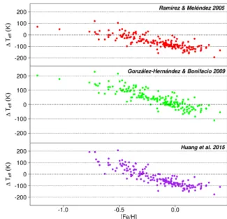
Figure 6 shows the residuals of the effective temperatures ob-tained with these various Teff versus V − Ks literature relations

with respect to the Teff derived through our ˆT versus G − Ks

fit. The differences stay mostly within ±100 K, but with a strong correlation with metallicity; these differences are mainly

explained by the various sources of effective temperatures together with the different treatment of the interstellar ex-tinction in each case. This correlation is stronger than that documented on the APOGEE DR13 release (see the corre-sponding discussion in Sect. 2.6). Applying the suggested correction still leads to a significant correlation with the resid-uals of the González Hernández & Bonifacio (2009) tempera-tures, although smaller. For users interested in working in the González Hernández & Bonifacio(2009) [GHB09] temperature scale, we found that, within the range of metallicity tested here, a simple linear relation allows the transformation Teff(GHB09) =

5040 ˆT+ 7 − 200 [Fe/H].

5. Red clump absolute magnitudes

To calibrate the absolute magnitudes of the RC, we selected a different sample of stars. Indeed, in order to avoid contamina-tion by the secondary red clump (see next Sect. 6), we made use only of stars within 1.93 < G − Ks < 2.3 and for which

M_Ks is brighter than −0.5 (similar as in Eq. (2)). As in Sect.2, we kept only low extinction stars (i.e. E(B − V)max< 0.01) with

σG < 0.01 and high photometric quality on the K band. The

sample contains 2482 stars. For each band we then applied the same photometric constraints as for the CC and TeffC

calibra-tions, previously specified in Sect.2.3.

Considering the strong contamination of the RC by the RGB bump and the variation of both the RC and RGB bump with colour, we did not estimate the RC absolute magnitude through a Gaussian fit to the magnitude distribution but through the mode of the distribution. The mode estimate is also less sensitive to the sample selection function. To model the colour dependency we looked for the maximum of Q(α, β), a kernel based distribu-tion funcdistribu-tion of the residuals Mλ− (α(G − Ks)+ β), with Mλthe

absolute magnitude of each particular band,

max (α,β) Q(α, β)= N X i=1 φ(α + β (G − Ks− 2.1) − Mλ) (5)

where the constant 2.1, the median of G − Ksof the sample,

al-lows us to centre the fit on the RC.

The kernel φ we used corresponds to a Gaussian model of the parallax errors converted in magnitude space (we neglected

(8)

Fig. 4.Empirical colour vs. G − Kscalibrations for B − Ks, G − J, g − r and g − i colour indices. The dash-dotted lines correspond to our calibration

at fixed metallicities (see legend). The colour of the points varies as a function of the metallicity. Diamonds correspond to the outliers removed at 3σ during the MCMC process. At the bottom of each calibration plot the residuals of the fit as a function of G − Ksand [Fe/H] are shown. All

plots are scaled to the same G − Kscolour and metallicity intervals.

here the photometric errors), i.e. φ = PM(M|M0)= P$($(M)|$0)

∂$

∂M (6)

φ(α + β (G − Ks) − Mλ) ∝ N($α,β,G, $, σ$) $α,β,mλ (7)

with $α,β,mλ= 10(α+β (G−Ks)−mλ−5)/5.

This method allows us to work directly with the parallaxes without selection in relative precision, avoiding the correspond-ing biases.

(9)

Table 2. Coefficients and range of applicability of the ˆT vs. G − Ks relation (top table) and the ˆT vs. G − Ks relation (bottom table), Y =

a0+ a1 X+ a2X2+ a3[Fe/H] + a4[Fe/H]2+ a5X[Fe/H].

Teff G − Ksrange [Fe/H] range a0 a1 a2 a3 a4 a5 RMS_[Teff(K)] %outliers N ˆ

T [1.6, 3.7] [−2.2, 0.4] 1.648 ± 0.027 −0.455 ± 0.023 0.054 ± 0.005 0.088 ± 0.012 0.001 ± 0.002 −0.026 ± 0.006 59 1.3 523 Colour Teffrange (K) [Fe/H] range a0 a1 a2 a3 a4 a5 RMS[G−Ks] %outliers N G − Ks [3603.7, 5207.7] [−2.2, 0.4] 13.554 ± 0.478 −20.429 ± 1.020 8.719 ± 0.545 0.143 ± 0.013 −0.0002 ± 0.009 − 0.05 1.3 523

Notes. We point out that ˆT= Teff/5040. The range of temperatures of the [ ˆT, G − Ks] calibration (second table) is given in Teff(not ˆT).

Fig. 5.Empirical normalised effective temperature vs. G − Ks

calibra-tion. The dash-dotted lines correspond to our calibration at fixed metal-licities (see legend). The colour of the points varies as a function of the metallicity. Diamonds correspond to the outliers removed at 3σ during the MCMC process. The residuals of the fit as a function of G − Ksand

[Fe/H] are shown at the bottom.

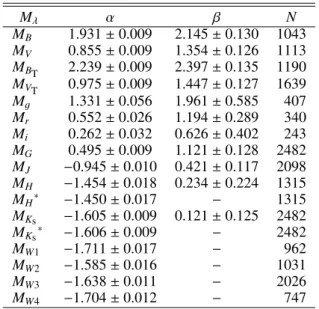
In Table 3 we summarise the results obtained with this method for 15 photometric bands. The initial uncertainties ob-tained through the maximum optimisation algorithm appeared underestimated (∼0.004). Indeed we saw that by changing the sample selection slightly, the results changed by more than the quoted errors. We provide in Table3the uncertainties by boot-strap instead.

We checked the degree of significance of the colour term for each relationship through a p-value test at 99% confidence level. We find a marginal dependence on colour for M_Ks (p-value of 0.004) and for MH(p-value of 0.002), negligible for MW1, MW2,

MW3 and MW4, and an important dependence for MG and the

other magnitudes. For those magnitudes for which there is no significant dependence we provide the results computed with β fixed to zero (indicated with “–” in the table). We also include in Table3the results obtained for M_Ksand MHwithout taking into

account their marginal dependence on colour (M_Ks = −1.606 ± 0.009, MH= −1.450 ± 0.017).

We checked the robustness of the mode estimate versus the selected sample. We found differences of 0.006 mag when se-lecting only stars with σ$/$ < 10% (1085 stars).

We determined similarly the mode of the RC M_Ks distri-bution according to the Padova isochrones, simulating an HR

Fig. 6.Residuals of the effective temperatures obtained through the

Teffvs. V − Kscalibrations ofRamírez & Meléndez(2005) (top panel,

red),González Hernández & Bonifacio (2009) (middle panel, green), and Huang et al. (2015) (bottom panel, purple). These residuals are shown with respect to the values derived with the ˆT vs. G − Ks fit of

this work for a sample of 179 APOGEE stars with high photometric quality and low interstellar extinction.

diagram with a constant star formation rate (SFR), aChabrier (2001) initial mass function (IMF), and a Gaussian metallicity distribution (0, 0.02). We obtained M_Ks = −1.660 ± 0.003, in agreement withBovy et al.(2014). We checked that indeed the mode is robust to changes in the SFR, the IMF, and the age-metalliticy ratio (AMR) hypothesis.

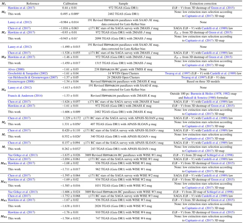
A summary of various absolute magnitude calibrations in the literature can be found in Table4, based on Table 1 ofGirardi (2016) and complemented with more recent studies. In this table we indicate, for comparison purposes, our result from Table3 assuming G − Ks colour equal to 2.1 when the external

cali-brations did not consider a colour effect while we found such a dependency.

We found general agreement with the M_Ks from previous works who mainly used H

_ipparcos

data. The M_Ks value of Alves (2000) is in the TMSS system (Bessell & Brett 1988), while the others, including this work, mainly used 2MASS data. However the quality flags considered to select the data are not the same in each case. Our M_Ks value of the mean RC K-band absolute magnitude appears to be slightly lower than inAlves (2000),Grocholski & Sarajedini(2002) andLaney et al.(2012), but higher than the values in van Helshoecht & Groenewegen (2007), Groenewegen (2008) and Francis & Anderson (2014). This value perfectly agrees with the last result ofHawkins et al. (2017) also using Gaia data but with a very different selec-tion funcselec-tion and handling of the extincselec-tion. As in this work,

(10)

Table 3. Coefficients of the absolute magnitude calibrations of the RC, Mλ= α + β (G − Ks− 2.1). Mλ α β N MB 1.931 ± 0.009 2.145 ± 0.130 1043 MV 0.855 ± 0.009 1.354 ± 0.126 1113 M_BT 2.239 ± 0.009 2.397 ± 0.135 1190 M_VT 0.975 ± 0.009 1.447 ± 0.127 1639 Mg 1.331 ± 0.056 1.961 ± 0.585 407 Mr 0.552 ± 0.026 1.194 ± 0.289 340 Mi 0.262 ± 0.032 0.626 ± 0.402 243 MG 0.495 ± 0.009 1.121 ± 0.128 2482 MJ −0.945 ± 0.010 0.421 ± 0.117 2098 MH −1.454 ± 0.018 0.234 ± 0.224 1315 MH∗ −1.450 ± 0.017 − 1315 M_Ks −1.605 ± 0.009 0.121 ± 0.125 2482 M_Ks∗ −1.606 ± 0.009 − 2482 MW1 −1.711 ± 0.017 − 962 MW2 −1.585 ± 0.016 − 1031 MW3 −1.638 ± 0.011 − 2026 MW4 −1.704 ± 0.012 − 747

Notes.(∗)_{Result without taking into account the marginal dependence}

on colour (p-value< 0.005)

Groenewegen(2008) also found a weak dependency of M_Ks on colour.

For MJ,Laney et al.(2012) found a slightly larger result with

respect to us. However, the source of photometric data is di ffer-ent from ours, and we have a much larger sample. Chen et al. (2017) used a much smaller sample and their value is even higher than that ofLaney et al.(2012), but the former result is still consistent with this work. We find perfect agreement with Hawkins et al.(2017) who also used a sample of Gaia stars. The same authors also calibrated MH, the results of which are in fair

agreement with our value.

Chen et al. (2017) also calibrated the APASS-SLOAN

gri absolute magnitudes using seismically determined RC stars from the Strömgren survey for Asteroseismology and Galactic Archaeology (SAGA). We find that the RC is less bright in all three magnitudes although within the errors bars.

As shown in Table4, for MW1 our result agrees with both

Chen et al.(2017) andHawkins et al.(2017), and it is marginally brighter than that ofYaz Gökçe et al.(2013). For MW2 we also

find good agreement withChen et al. (2017), however the dif-ferences are larger with respect toHawkins et al.(2017), as they have already pointed out in their article. We have indeed found important variations depending on the sample selection criteria. In particular, by considering only the high photometric quality flag (i.e. qph = A) and no cut in the observed magnitude, we obtained MW2 = −1.68 ± 0.01 with a strong correlation with

colour. By removing the saturated stars (Cotten & Song 2016), as described in Sect.2.3, this dependence with colour becomes negligible, as it is for the other WISE bands, and the peak is much fainter. This may explain the too bright value found by Hawkins et al.(2017).

With MW3 all the works are consistent with the exception

of Chen et al. (2017) who obtained a brighter value. And for MW4 our result is fainter than that found for the first time by

Hawkins et al.(2017).

Finally,Hawkins et al.(2017) also provided the first calibra-tion of MG, based on a hierarchical probabilistic model. In this

work we provide a different approach by directly using the mode of the distribution and with a larger sample of data. Their G

absolute magnitude is somewhat brighter. As mentioned above, with our method we also find a strong dependence on colour. This may explain the difference between both estimations, to-gether with the fact that they corrected the reddening by deriv-ing the extinction coefficients through the nominal Gaia G band. The updated extinction coefficients will be found in Danielski et al. (in prep.).

Besides the parallax accuracy and various sources of photo-metric information, one of the main differences between these estimates is the handling of the interstellar extinction. Alves (2000), Stanek & Garnavich (1998), Girardi et al. (1998), and Laney et al.(2012) assumed no reddening, while the other au-thors corrected their magnitudes using and combining different interstellar laws and/or maps. It is clear that our sample selec-tion based on low extincselec-tion stars introduces as well a bias in all our calibrations, although minimally. Indeed, the reddening cut at E(B − V)max < 0.01 corresponds to a maximum

overes-timation of the absolute magnitude of about 0.02 mag in the G band, while about 0.003 mag in the K band (see Danielski et al., in prep.).

The discrepancies among the other estimates may also be justified by the different methods used: most of the authors con-sidered a Gaussian fit, while here we used the mode of the distribution.

6. The TGAS red clump HR diagram

Figure7shows the TGAS HR diagram for red giant stars for ab-solute magnitudes in the G and K photometric bands. We used stars listed in TableA.1(see AppendixA) with low extinction (E(B − V)max < 0.015), 10% parallax precision, σG < 0.01,

and 2MASS JK high photometric quality. In both cases the RC is easily detected. However other features may also be ob-served. Indeed, on the bluest part of the RC we can see a small overdensity belonging to the secondary red clump (Girardi et al. 1998;Girardi 1999), a group of still metal-rich but younger (i.e. slightly more massive) stars that extend the RC to fainter mag-nitudes (up to 0.4 mag fainter). On the red side of the clump and below it, we find the red giant branch bump (RGB bump or RGBB), another overdensity of slightly more massive stars than the RC, which causes a peak (bump) in the luminosity function (seeChristensen-Dalsgaard(2015) for a review on this CMD feature).

On the same diagrams we also overplotted the absolute mag-nitude calibrations obtained in previous Sect.5(Table3).

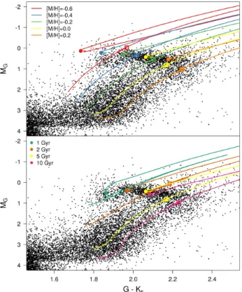
In Fig. 8 we show the RC HR diagram again but with the Padova isochrones (Bressan et al. 2012, Parsec 2.7) at di ffer-ent metallicities (top panel) and at different ages (bottom panel) overplotted in different colours. We use the original Te_fffrom the

isochrones and applied our G − Ksversus ˆTcalibration (Table2)

to derive the colour G − Ks.

We may see that while the position of the RC seems to nicely fit the isochrones, the RGB bump is slightly too bright in the isochrones. Following the process in Sect.5, we found a di ffer-ence of −0.07 mag between the Padova RC and the TGAS RC, and about 0.2 mag for the RGB bump.

7. Conclusions

Using the first Gaia Data Release parallaxes and photometry, the new 3D interstellar extinction map ofCapitanio et al.(2017), the 2MASS catalogue and the last APOGEE release (DR13), a complete photometric calibration including colours (spread from

(11)

Table 4. Comparison of the Mλof this work with other determinations in the literature.

Mλ Reference Calibration Sample Extinction correction MG

Hawkins et al.(2017) 0.44 ± 0.01 972 TGAS (Gaia DR1) E(B − V) from 3D dustmap ofGreen et al.(2015) This work 0.495 ± 0.009∗ _{2482 TGAS (Gaia DR1)} None: low extinction stars selection according

toCapitanio et al.(2017) 3D map

MJ

Laney et al.(2012) −0.984 ± 0.014 191 Revised Hipparcosparallaxes with SAAO JK mag, None data corrected for Lutz-Kelker bias

Chen et al.(2017) −1.016 ± 0.063 .171 RC stars of the SAGA survey with 2MASS J mag SAGA E(B − V) withCardelli et al.(1989) law

Hawkins et al.(2017) −0.93 ± 0.01 972 TGAS (Gaia DR1) with 2MASS J mag EB − Vfrom 3D dustmap ofGreen et al.(2015) This work −0.945 ± 0.01∗ _{2098 TGAS (Gaia DR1) with 2MASS J mag} None: low extinction stars selection according

MH

Laney et al.(2012) −1.490 ± 0.015 191 Revised Hipparcosparallaxes with SAAO JK mag, None data corrected for Lutz-Kelker bias

Chen et al.(2017) −1.528 ± 0.055 .171 RC stars of the SAGA survey with 2MASS J mag SAGA E(B − V) withCardelli et al.(1989) law

Hawkins et al.(2017) −1.46 ± 0.01 972 TGAS (Gaia DR1) with 2MASS J mag EB − Vfrom 3D dustmap ofGreen et al.(2015) This work −1.450 ± 0.017 1315 TGAS (Gaia DR1) with 2MASS J mag None: low extinction stars selection according

MK

Alves(2000) −1.61 ± 0.03 238 HipparcosRC giants with TMSS K mag None

Grocholski & Sarajedini(2002) −1.61 ± 0.04 14 WYIN Open Clusters Twarog et al.(1997) E(B − V) withCardelli et al.(1989) law

van Helshoecht & Groenewegen(2007) −1.57 ± 0.05 24 2MASS Open Clusters Twarog et al.(1997) E(B − V) data

Groenewegen(2008) −1.54 ± 0.04 Revised Hipparcosparallaxes with 2MASS K mag Based on three 3D models

Laney et al.(2012) −1.613 ± 0.015 191 Revised Hipparcosparallaxes with SAAO K mag, None data corrected for Lutz-Kelker bias

Francis & Anderson(2014) −1.53 ± 0.01 Revised Hipparcosparallaxes with 2MASS K mag Outside 100 pc:Burstein & Heiles(1978,1982) map andBahcall & Soneira(1980) formulae

Chen et al.(2017) −1.626 ± 0.057 .171 RC stars of the SAGA survey with 2MASS K band SAGA E(B − V) withCardelli et al.(1989) law

Hawkins et al.(2017) −1.61 ± 0.01 972 TGAS (Gaia DR1) with 2MASS K mag E(B − V) from 3D dustmap ofGreen et al.(2015) This work −1.606 ± 0.009 2482 TGAS (Gaia DR1) with 2MASS K mag None: low extinction stars selection according

toCapitanio et al.(2017) 3D map Mg

Chen et al.(2017) 1.229 ± 0.172 .171 RC stars of the SAGA survey with APASS-SLOAN g mag SAGA E(B − V) withCardelli et al.(1989) law This work 1.331 ± 0.056∗ _{407 TGAS (Gaia DR1) with APASS-SLOAN g mag} None: low extinction stars selection according

toCapitanio et al.(2017) 3D map Mr

Chen et al.(2017) 0.420 ± 0.110 .171 RC stars of the SAGA survey with APASS-SLOAN r mag SAGA E(B − V) withCardelli et al.(1989) law This work 0.552 ± 0.026∗ _{340 TGAS (Gaia DR1) with APASS-SLOAN r mag} None: low extinction stars selection according

toCapitanio et al.(2017) 3D map Mi

Chen et al.(2017) 0.157 ± 0.094 .171 RC stars of the SAGA survey with APASS-SLOAN i mag SAGA E(B − V) withCardelli et al.(1989) law This work 0.262 ± 0.032∗ _{243 TGAS (Gaia DR1) with APASS-SLOAN i mag} None: low extinction stars selection according

MW1

Yaz Gökçe et al.(2013) −1.635 ± 0.026 3889 Revised HipparcosRC parallaxes with WISE W1 mag E(B − V) from 2D map ofSchlegel et al.(1998)

Chen et al.(2017) −1.694 ± 0.061 .171 RC stars of the SAGA survey with WISE W1 mag SAGA E(B − V) withCardelli et al.(1989) law

Hawkins et al.(2017) −1.68 ± 0.02 936 TGAS (Gaia DR1) with WISE W1 mag E(B − V) from 3D dustmap ofGreen et al.(2015) This work −1.711 ± 0.017 962 TGAS (Gaia DR1) with WISE W1 mag None: low extinction stars selection according

toCapitanio et al.(2017) 3D map MW2

MW3

Yaz Gökçe et al.(2013) −1.606 ± 0.024 3889 Revised HipparcosRC parallaxes with WISE W3 mag E(B − V) from 2D map ofSchlegel et al.(1998)

toCapitanio et al.(2017) 3D map MW4

Notes.(∗)_{Result from Table}₃_{assuming G − K}

scolour equal to 2.1.

visual to infrared wavelengths), absolute magnitudes, spectro-scopic metallicities, and homogeneous effective temperatures is provided in this work for solar neighbourhood RC stars. We have made use of high photometric quality data from the Gaia, John-son, 2MASS, H

_ipparcos

, Tycho-2, APASS-SLOAN, and WISE photometric systems.

A robust MCMC method accounting for all

vari-able uncertainties was developed to derive 20 accurate metallicity-dependent colour–colour relations and the ˆT versus G − Ks and G − Ks versus ˆT fits (with ˆT the normalised

effective temperature, ˆT = Teff/5040). We checked that the

effective temperature calibration is compatible with those from Ramírez & Meléndez(2005),González Hernández & Bonifacio (2009) andHuang et al.(2015) within the metallicity and colour ranges of applicability.

We also derived the absolute magnitudes for the TGAS RC on 15 photometric bands (including MGand MKs) through a

ker-nel based magnitude distribution method and with the largest high quality dataset used so far for an absolute magnitude cal-ibration of the RC. We obtained a small dependence on colour for M_Ks and MH, which is not significant for MW1, MW2, MW3

and MW4, but important for MGand the other magnitudes.

All these photometric relationships will be improved in later Gaiareleases and extended to other photometric bands, when larger RC samples will be available.

We presented a dereddened TGAS HR diagram for the RC region, in which we can already easily identify other fea-tures of red giant stars, such as the secondary RC and the RGB Bump. By using our calibrations we could compare the Padova isochrones with the TGAS HR diagram and found good

(12)

Fig. 7.TGAS HR diagram of the RC region for the MG(top) and the

MKs (bottom) absolute magnitudes, using stars with E(B − V)max <

0.015, 10% parallax precision, σG < 0.01, and 2MASS JKs high

photometric quality. The location of the secondary red clump and the RGB bump features are easily observed on the diagram. We have high-lighted them in blue and red, respectively. The yellow line shows the absolute magnitude calibration obtained in this work.

agreement with the RC location on the diagram, although the RGB bump appears too bright in the isochrones.

The photometric calibrations presented here are being used to derive kG, the interstellar extinction coefficient in the G band

(Danielski et al., in prep.), and to provide photometric interstellar extinctions of large surveys such as APOGEE to be included in the next release of the new 3D extinction map ofCapitanio et al. (2017).

In summary, this work used the high quality of the Gaia DR1 data to calibrate the Gaia RC. In turn, these calibrations can be used as the second rung of the cosmic distance ladder. In-deed, together with asteroseismic constraints, we can now derive the distance modulus of a large sample of RC stars. By choos-ing RC stars distant enough so that their estimated distance un-certainty is better than the Gaia parallax precision, these stars may be used to check the zero point of the Gaia parallaxes and their precision (Arenou et al. 2017). This is already being ap-plied within the Gaia Data Release 2 verification process.

Acknowledgements. L.R.-D. acknowledges financial support from the Centre National d’Etudes Spatiales (CNES) fellowship programme. This work has made use of data from the European Space Agency (ESA) mission Gaia (https: //www.cosmos.esa.int/gaia), processed by the Gaia Data Processing and Analysis Consortium (DPAC, https://www.cosmos.esa.int/web/gaia/ dpac/consortium). Funding for the DPAC has been provided by national in-stitutions, in particular the institutions participating in the Gaia Multilateral Agreement. This publication makes use of data products from the Two Mi-cron All Sky Survey, which is a joint project of the University of Massachusetts and the Infrared Processing and Analysis Center/California Institute of Tech-nology, funded by the National Aeronautics and Space Administration and the

Fig. 8. Padova isochrones overlaid on the Gaia DR1 HRD. Top: isochrones for an age of 5 Gyr and various metallicities are shown. Bottom: isochrones for a solar metallicity and various ages are shown. Circles correspond to the RC location and squares correspond to the RGB bump.

National Science Foundation. L.R.-D. acknowledges support from Agence Na-tionale de la Recherche through the STILISM project (ANR-12-BS05-0016-02). This research has also made use of VizieR databases operated at the Centre de Données astronomiques de Strasbourg (CDS) in France.

References

Adibekyan, V. Z., Sousa, S. G., Santos, N. C., et al. 2012,A&A, 545, A32

Alves, D. R. 2000,ApJ, 539, 732

Alves, S., Benamati, L., Santos, N. C., et al. 2015,MNRAS, 448, 2749

Arenou, F., Luri, X., Babusiaux, C., et al. 2017,A&A, 599, A50

Aringer, B., Girardi, L., Nowotny, W., Marigo, P., & Bressan, A. 2016,MNRAS, 457, 3611

Bahcall, J. N., & Soneira, R. M. 1980,ApJS, 44, 73

Bensby, T., Feltzing, S., & Oey, M. S. 2014,A&A, 562, A71

Bessell, M. S., & Brett, J. M. 1988,PASP, 100, 1134

Bovy, J., Nidever, D. L., Rix, H.-W., et al. 2014,AJ, 790, 127

Bressan, A., Marigo, P., Girardi, L., et al. 2012,MNRAS, 427, 127

Bruntt, H., Basu, S., Smalley, B., et al. 2012,MNRAS, 423, 122

Burstein, D., & Heiles, C. 1978,Astrophys. Lett., 19, 69

Burstein, D., & Heiles, C. 1982,AJ, 87, 1165

Capitanio, L., Lallement, R., Vergely, J. L., Elyajouri, M., & Monreal-Ibero, A. 2017,A&A, 606, A65

Cardelli, J. A., Clayton, G. C., & Mathis, J. S. 1989,AJ, 345, 245

Chabrier, G. 2001,ApJ, 554, 1274

Chen, Y. Q., Casagrande, L., Zhao, G., et al. 2017,ApJ, 840, 77

Christensen-Dalsgaard, J. 2015,MNRAS, 453, 666

Cotten, T. H., & Song, I. 2016,ApJS, 225, 15

Cutri, R. M., Skrutskie, M. F., van Dyk, S., et al. 2003, VizieR Online Data Catalog: II/246

da Silva, R., Milone, A. d. C., & Rocha-Pinto, H. J. 2015,A&A, 580, A24

De Pascale, M., Worley, C. C., de Laverny, P., et al. 2014,A&A, 570, A68

Evans, D. W., Riello, M., De Angeli, F., et al. 2017,A&A, 600, A51

Fabricius, C., Høg, E., Makarov, V. V., et al. 2002,A&A, 384, 180

Francis, C., & Anderson, E. 2014,MNRAS, 441, 1105

Gaia Collaboration (Brown, A. G. A., et al.) 2016,A&A, 595, A2

García Pérez, A. E., Allende Prieto, C., Holtzman, J. A., et al. 2016,AJ, 151, 144

(13)

Girardi, L. 1999, in the evolution of the Milky Way: stars versus clusters (Kluwer Academic Publishers)

Girardi, L. 2016,ARA&A, 54, 95

Girardi, L., Groenewegen, M. A. T., Weiss, A., & Salaris, M. 1998,MNRAS, 301, 149

González Hernández, J. I., & Bonifacio, P. 2009,A&A, 497, 497

Green, G. M., Schlafly, E. F., Finkbeiner, D. P., et al. 2015,ApJ, 810, 25

Grocholski, A. J., & Sarajedini, A. 2002,AJ, 123, 1603

Groenewegen, M. A. T. 2008,A&A, 488, 935

Hawkins, K., Leistedt, B., Bovy, J., & Hogg, D. W. 2017,MNRAS, 471, 722

Henden, A. A., Templeton, M., Terrell, D., et al. 2016, VizieR Online Data Catalog: II/336

Høg, E., Fabricius, C., Makarov, V. V., et al. 2000,A&A, 355, L27

Holtzman, J. A., Shetrone, M., Johnson, J. A., et al. 2015,AJ, 150, 148

Huang, Y., Liu, X.-W., Yuan, H.-B., et al. 2015,MNRAS, 454, 2863

Jofré, E., Petrucci, R., Saffe, C., et al. 2015,A&A, 574, A50

Jordi, C., Gebran, M., Carrasco, J. M., et al. 2010,A&A, 523, A48

Kovtyukh, V. V., Soubiran, C., Bienaymé, O., Mishenina, T. V., & Belik, S. I. 2006,MNRAS, 371, 879

Kunder, A., Kordopatis, G., Steinmetz, M., et al. 2017,AJ, 153, 75

Lallement, R., Vergely, J.-L., Valette, B., et al. 2014,A&A, 561, A91

Laney, C. D., Joner, M. D., & Pietrzynski, G. 2012, VizieR Online Data Catalog: J/MNRAS/419/1637

Lindegren, L., Lammers, U., Bastian, U., et al. 2016,A&A, 595, A4

Luck, R. E. 2015,AJ, 150, 88

Luo, A.-L., Zhao, Y.-H., Zhao, G., et al. 2016, VizieR Online Data Catalog: V/149

Maldonado, J., & Villaver, E. 2016,A&A, 588, A98

Marrese, P. M., Marinoni, S., Fabrizio, M., & Giuffrida, G. 2017,A&A, 607, A105

Martell, S. L., Sharma, S., Buder, S., et al. 2017,MNRAS, 465, 3203

Morel, T., Miglio, A., Lagarde, N., et al. 2014,A&A, 564, A119

Mortier, A., Santos, N. C., Sousa, S. G., et al. 2013,A&A, 558, A106

Paczynski, B., & Stanek, K. Z. 1998,ApJ, 494, L219

Perryman, M., Agency, E. S., & Consortium, F. 1997, The Hipparcosand Tycho Catalogues: The Hipparcoscatalogue, ESA SP (ESA Publications Division) Plummer, M. 2008,Biostatistics, 9, 523

Pourbaix, D., Tokovinin, A. A., Batten, A. H., et al. 2004,A&A, 424, 727

Pourbaix, D., Tokovinin, A. A., Batten, A. H., et al. 2009, VizieR Online Data Catalog: B/sb9

Puzeras, E., Tautvaisiene, G., Cohen, J. G., et al. 2010,MNRAS, 408, 1225

Ramírez, I., & Meléndez, J. 2005,ApJ, 626, 446

Ramirez, I., Melendez, J., & Asplund, M. 2013, VizieR Online Data Catalog: J/A+A/561/A7

Ramírez, I., Bajkova, A. T., Bobylev, V. V., et al. 2014a,ApJ, 787, 154

Ramírez, I., Meléndez, J., Bean, J., et al. 2014b,A&A, 572, A48

Saguner, T., Munari, U., Fiorucci, M., & Vallenari, A. 2011,A&A, 527, A40

Schlafly, E. F., & Finkbeiner, D. P. 2011,ApJ, 737, 103

Schlegel, D. J., Finkbeiner, D. P., & Davis, M. 1998,ApJ, 500, 525

SDSS Collaboration 2017,ApJS, 233, 25

Soubiran, C., Le Campion, J.-F., Brouillet, N., & Chemin, L. 2016,A&A, 591, A118

Stanek, K. Z., & Garnavich, P. M. 1998,ApJ, 503, L131

Takeda, Y., Sato, B., & Murata, D. 2008,PASJ, 60, 781

Thygesen, A. O., Frandsen, S., Bruntt, H., et al. 2012,A&A, 543, A160

Twarog, B. A., Ashman, K. M., & Anthony-Twarog, B. J. 1997,AJ, 114, 2556

Udalski, A. 2000,ApJ, 531, L25

Valentini, M., & Munari, U. 2010,A&A, 522, A79

van Helshoecht, V., & Groenewegen, M. A. T. 2007,A&A, 463, 559

van Leeuwen, F., Evans, D. W., De Angeli, F., et al. 2017,A&A, 599, A32

Wright, E. L., Eisenhardt, P. R. M., Mainzer, A. K., et al. 2010,AJ, 140, 1868

Yaz Gökçe, E., Bilir, S., Öztürkmen, N. D., et al. 2013,New Astron., 25, 19

Zieli´nski, P., Niedzielski, A., Wolszczan, A., Adamów, M., & Nowak, G. 2012,

A&A, 547, A91

Appendix A: Low extinction TGAS HR Catalogue at CDS

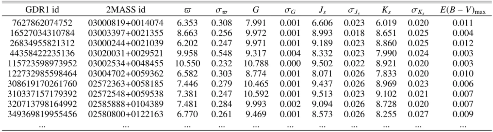
TableA.1contains a few rows of the low extinction TGAS HRD compilation used in this work. The full table is available in VizieR.

The catalogue includes 142 996 stars with – Gaia DR1 and 2MASS identifiers.

– Gaia DR1 parallaxes with precision better than 10%. – Gaia DR1 G magnitude with uncertainties lower than

0.01 mag.

– 2MASS J and Ksphotometric bands with high quality (i.e.

flag q2M= “A.A”) and uncertainties lower than 0.03 mag – Reddening E(B − V)max< 0.015 according to the Capitanio

et al. (2017) 3D interstellar extinction map, and the Schlegel et al.(1998) 2D map for stars for which the distance goes beyond the 3D map borders.

Table A.1. First rows of the low extinction and high photometric and astrometric quality TGAS HRD catalogue.

GDR1 id 2MASS id $ σ$ G σG Js σJs Ks σKs E(B − V)max

7627862074752 03000819+0014074 6.353 0.308 7.991 0.001 6.606 0.023 6.019 0.020 0.011 16527034310784 03003397+0021355 8.663 0.256 9.972 0.001 8.993 0.018 8.651 0.025 0.004 26834955821312 03000244+0021039 6.202 0.247 9.971 0.001 9.189 0.023 8.860 0.025 0.012 44358422235136 03020031+0029521 9.958 0.548 9.317 0.004 8.332 0.023 7.990 0.024 0.003 115723598973952 03002534+0048455 10.550 0.232 10.788 0.000 9.502 0.022 8.921 0.020 0.003 122732985598464 03004702+0059362 6.582 0.303 8.774 0.001 8.071 0.026 7.833 0.020 0.010 308619170261760 02572363+0058185 7.446 0.279 10.465 0.001 9.437 0.026 8.969 0.023 0.006 310337157179392 02572548+0059538 7.381 0.247 10.592 0.001 9.513 0.023 9.102 0.021 0.007 320713798164992 02585888+0104389 7.481 0.284 9.993 0.002 9.094 0.026 8.728 0.020 0.007 349369819955456 02580800+0122163 6.770 0.261 9.469 0.001 8.573 0.026 8.255 0.027 0.009 ... ... ... ... ... ... ... ... ... ... ...