Designing robust railroad blocking plans

Designing Robust Railroad Blocking Plans

by

Hong Jin

Submitted to the Department of Civil and Environmental Engineering

in partial fulfillment of the requirements for the degree of

Doctor of Philosophy in Transportation and Logistics Systems

at the

MASSACHUSETTS INSTITUTE OF TECHNOLOGY

@

Massachusetts

Author...

-June 1998,

Institute-f Thchnology 1998.

Anfrights reserved.

Environmental Engineering

June 30, 1998

Certified by ...

Cynthia Barnhart

Associate Professor of Civil and Environmental Engineering

Thesis Supervisor

Accepted by

...

...

Joseph.

Sussman

Joseph Sussman

MASSACHUSETTS INSTITUTE

OF TECHNOLOGY

OCT 2 6 1998

LIBRARIES

Designing Robust Railroad Blocking Plans

by

Hong Jin

Submitted to the Department of Civil and Environmental Engineering on June 30, 1998, in partial fulfillment of the

requirements for the degree of

Doctor of Philosophy in Transportation and Logistics Systems

Abstract

On major domestic railroads, a typical general merchandise shipment, or commodity, may pass through many classification yards on its route from origin to destination. At these yards, the incoming traffic, which may consist of several shipments, is re-classified (sorted and grouped together) to be placed on outgoing trains. On average, each reclassification results in an one day delay for the shipment. In addition, the classification process is labor and capital intensive. To prevent shipments from being reclassified at every yard they pass through, several shipments may be grouped to-gether to form a block. The blocking problem consists of choosing the set of blocks to be built at each terminal (the blocking plan) and assigning each commodity to a series of blocks that will take it from origin to destination. It is one of the most important problems in railroad freight transportation since a good blocking plan can reduce the number of reclassifications of the shipments, thus reducing operating costs and delays associated with excess reclassifications.

We provide a variety of model formulations that attain the minimum costs for different problem instances. The deterministic model identifies the blocking plan for the problems with certainty in problem inputs. Static stochastic models provide blocking plans that are feasible for all possible realizations of uncertainties in demand and supply. Dynamic stochastic models generate blocking plans that balance flow costs and plan change costs for possible realizations of uncertainties.

We adopt Lagrangian relaxation techniques to decompose the resulting huge mixed integer programming models into two smaller subproblems. This reduces storage requirements and computational efforts to solve these huge problems. We propose other enhancements to reduce computational burden, such as adding a set of valid inequalities and using advanced start dual solutions. These enhancements help tighten the lower bounds and facilitate the generation of high quality feasible solutions.

We test the proposed models and solution approaches using the data from a major railroad. Compared to current blocking plans, the solutions from our model reduce the total number of classifications significantly, leading to potential savings of millions of dollars annually. We also investigate various problem aggregation techniques to determine the appropriate ways of generating satisfactory blocking plans with

differ-ent levels of computational resources. We illustrate the benefits of robust planning by comparing the total costs of our robust plans with those of our deterministic plans. The experiments show that the the realized costs can be reduced by around 50% using robust blocking plans.

Thesis Supervisor: Cynthia Barnhart

Acknowledgments

Firstly, I would like to express my great appreciation for my advisor, Professor Cyn-thia Barnhart. Her constant guidance, encouragement and support are so valuable that the thesis is not possible without her direction.

Deep appreciation is extended to my committee members. Professors Joseph Suss-man and Yosef Sheffi provide insightful discussions and suggestions that inspire Suss-many topics in my thesis. Professor Pamela Vance from Auburn University tirelessly travels to participate in the committee meetings, her suggestions and comments greatly help in solution algorithm development.

Also, I would like to take this opportunity to thank Carl Martland, my advisor when I was in the MIT Rail Group. His direction, encouragement lead me from a student to a researcher.

I thank UPS foundation and CSX Transportation for sponsoring my research. Raja Kasilingam, Adriene Bailey, Dharma Acharya, Yen Shan and James Lyvers from CSXT provide constant support and information on railroad operations. Harry Newton from Air Force Academy gives me a big help at the beginning of this study. I want to thank my friends and office-mates in 5-012, Niranjan Krishnan, Francisco Jauffred, Andy Armacost and Daeki Kim for their useful discussions and unselfish help. I acknowledge my fellow students in CTS, Qi Yang, John Bowman, Yan Dong, Chris Capalice, Owen Chen, Joan Walker, Scott Ramming, Jon Bottom, Kazi Ahmed, Winston Guo, Zhaopu Si, Qian Ma, William Robert, Xing Yang, Julie Wei, Fang Lu and Yiyi He for their friendship.

Last but not least, I would like to express gratitude to my family, my parents for their affection and support, my wife, Dongyan Ma, her understanding, patience and support.

Contents

1 Introduction 10

1.1 Railroad Tactical Planning ... ... 10

1.2 The Railroad Blocking Problem ... .. 12

1.2.1 Problem Introduction ... 12

1.2.2 Significance of Blocking Problem . ... 13

1.2.3 Previous Blocking Research . ... 14

1.2.4 The Blocking Problem with Uncertainty . ... 15

1.3 Review of Related Literature ... ... 18

1.3.1 Network Design ... 18

1.3.2 Stochastic Optimization ... 19

1.4 Thesis Outline ... .. . ... ... 21

2 Railroad Blocking with Deterministic Data 22 2.1 Network Design Models ... . . . . . 22

2.1.1 A Generalized Node-Arc Formulation . ... 22

2.1.2 A Path Formulation for Budget Network Design ... 25

2.1.3 Forcing Constraints ... 27

2.2 A Blocking Model with Deterministic Parameters . ... 27

2.2.1 Rail Blocking Network ... . 28

2.2.2 Model Formulation ... 29

2.3 Solution Approach ... .. 30

2.3.1 Lagrangian Relaxation ... 30

2.3.3 Lower Bound . . . . . . . . . . . .. 2.3.4 Upper Bound . . . . . . . . . . ..

2.3.5 Dual Ascent Processing . . . .. 2.4 Summary . ...

3 Railroad Blocking with Deterministic Data: A Case

3.1 Introduction . ... 3.2 Problem Data ... . ... 3.3 Problem Aggregation Schemes ...

3.3.1 Node-Based Aggregation . . . . 3.3.2 Route-Based Aggregation . . . .

3.3.3 Commodity-Based Aggregation . . . . 3.3.4 Comparison of Aggregation Schemes . . . . . 3.4 Problem Aggregation Case Studies . . . . 3.4.1 Implementation Details . . . . 3.4.2 Node-Based Aggregation Case Study . . . . . 3.4.3 Route-Based Aggregation Case Study . . . . . 3.4.4 Commodity-Based Aggregation Case Study

3.4.5 Computer Storage Requirements . . . .

3.4.6 Comparison to Current Operations . . . . 3.5 Real Time Blocking Plan Generation . . . . 3.6 Efficiency Enhancements . . . . 3.7 Volume Constraints in the Blocking Problem . . . . . 3.8 Sum m ary .... .. . .. . . . .. .. ... ... 4 The 4.1 4.2 . 38 . 39 * 43 * 45 Study ... . 49 ... . 50 . . . . . 51 . . . . . 52 . . . . . 53 . . . . . 54 . . . . . 54 . . . . . 54 . . . . . 55 . . . . . 61 . . . . . 64 . . . . . 66 . . . . . 69 . . . . . 69 . . . . . 72 . . . . . 73 ... . 74

Railroad Blocking Problem with Stochastic Inputs Uncertainties in the Railroad Blocking Problem . . . . Robustness and Robust Planning . . . . 4.2.1 Robustness Definition . . . . 4.2.2 Mathematical Formulations for Robustness . . . . . 4.2.3 Static vs. Dynamic Plans . . . . 76 . . . 76 . . . 78 . . . 78 . . . 80 81

4.2.4 Literature Review . . . . ..

4.3 Static Blocking Models ...

4.3.1 Static Worst-Case Model . . . ... 4.3.2 Static Expected Performance Model . . . . 4.4 Dynamic Expected Performance Blocking Models

4.4.1 Quadratic Dynamic Model . . . ... 4.4.2 Linear Dynamic Model . . . . ..

4.5 Summary ... ...

5 Robust Railroad Blocking: A Case Study

5.1 Alternative Blocking Plans . . . . 5.1.1 Static Blocking Plans ...

5.1.2 Dynamic Blocking Plans . . . . 5.2 Implementation Issues ...

5.2.1 Daily Variations in Demand . . . . 5.2.2 Plan Change Costs ...

5.2.3 Convergence Criteria ... 5.3 Computational Results ...

5.3.1 Single-Scenario Blocking Problems . . . .

5.3.2 Single-Scenario Blocking Plan Evaluation . 5.3.3 Robust Planning Improvements . . . . 5.3.4 Robust Planning with Limited Scenarios . 5.3.5 Simulation Case Study ...

5.4 Sum m ary ...

6 Contributions and Future Directions

6.1 Contributions ... 6.2 Future Directions ... 6.2.1 Model Development ... 6.2.2 Algorithmic Development . . . . 6.2.3 Application Context ... . . . . . . . . . 82 . . . . 83 . . . . . . . 84 . . . . . . . . . 87 . . . . . 88 . . . . . . 89 . . . . . 92 . . . . .. . 96 97 . . . . . 97 . . . . 97 . . . . . 98 . . . . 99 . . . . . 99 . . . . 100 . . . . 100 . . . . 101 . . . . 101 . . . . . 101 . . . . . 103 . . . . 108 . . . . 112 . . . . 117 118 . . . . 118 . . . . 119 . . . . 119 . . . . 120 . . . . 120

List of Figures

1-1 An Example of Blocking Path vs. Physical Route . ... 13

2-1 Column Generation Procedure for FLOW . ... 33

2-2 Branch-and-Cut Procedure for BLOCK . ... 35

2-3 Lagrangian Relaxation Approach for Blocking Problem ... 36

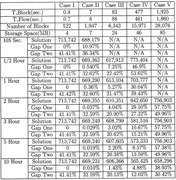
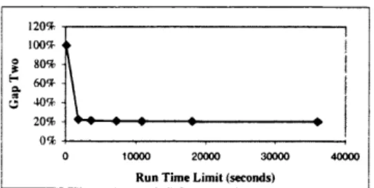
3-1 Best Feasible Solutions under Different Run Time Limits ... 58

3-2 Best Solution Profiles for Different Node Aggregation Levels .... . 60

3-3 Solution Values under Storage Space Constraints . ... 67

5-1 Realized Costs vs. Planned Costs for Static Plans Based on Single Scenarios . . . .. . . . 103

5-2 Cost Comparisons for Different Plans ... 105

5-3 Impacts of Scenario Selection on Realized Costs . ... 106 5-4 Realized Costs Comparisons for Static Plans Based on Single Scenarios 110 5-5 Realized Cost Comparisons for Dynamic Plans Based on Single Scenarios 111 5-6 Realized Cost Comparisons for Plans with Different Scenario Selection 113

List of Tables

3.1 Levels of Node-Based Aggregation and Problem Sizes . ... 56

3.2 Computational Results for Node-Based Aggregation . ... 57

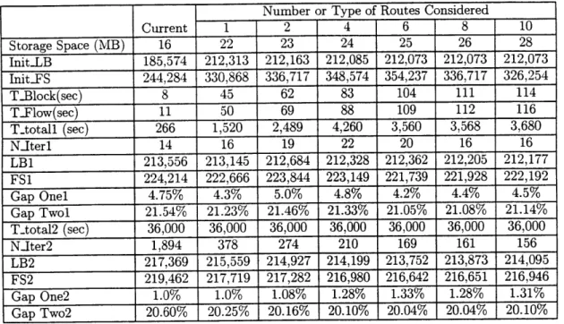
3.3 Computational Results for Route-Based Aggregation . ... 62

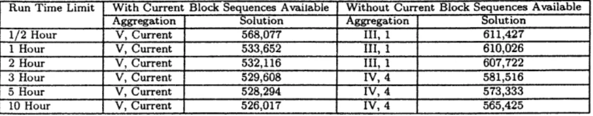
3.4 Appropriate Level of Aggregation and Solution . ... 64

3.5 Computational Results for Commodity-Based Aggregation ... 65

3.6 Appropriate Level of Aggregation and Solution Value with Storage Constraints ... .. ... .. ... ... ... 67

3.7 Model Solution vs. Current Practice . ... 69

3.8 "One-Shot" Feasible Plan Generation Comparisons . ... 71

3.9 Computational Results Comparisons on Medium Level Aggregate Net-w ork .. . . 73

3.10 Comparisons With and Without Car Volume Constraints ... 74

5.1 Daily Demand Variations in a Representative Week ... 100

5.2 Network Design Solutions Under a Single-Scenario ... 101

5.3 Plan Change Cost Assumptions in Robust Blocking Plans ... 107

5.4 Robust Plans under Different Change Cost Assumptions ... 107

5.5 Realized vs. Planned Costs for Daily Demand Scenarios ... 113 5.6 Comparisons of Realized Costs with Different Static Blocking Plans . 115 5.7 Comparisons of Realized Costs with Different Dynamic Blocking Plans 117

Chapter 1

Introduction

1.1

Railroad Tactical Planning

Railroad operations planning can be categorized according to Assad (1980) as Strate-gic, Tactical, or Operational. Strategic planning deals with long-term (usually in years) decisions on investments, marketing and network design including train ser-vices and schedules, capacity expansion, track abandonment and facility location. Tactical planning focuses on effective allocation of existing resources over medium-term planning horizons ranging from one month to one year. Operational planning, in a dynamic environment, manages the day-to-day activities, such as train timetable, empty car distribution, track scheduling and yard receiving/dispatching policies.

In strategic planning, railroads make up long-term business strategies, which usu-ally involve major capital investments. These strategies include:

* Network Design and Improvement laying out the network coverage and service range;

* Terminal Location and Capacity selecting the terminals and their func-tionality on the network, and equipping the functional yards with adequate resources;

* Service Planning and Differentiation setting the target market and service standards for various traffic with different priority; and

* Merger and Acquisition expanding network coverage and business by

com-bined effort and cooperation from other companies.

In tactical planning, railroads determine how to move the traffic from origins to destinations using available system resources. The results of tactical planning are operating plans, including

* Blocking Plans dictating which blocks (i.e. groups of shipments to be classified

as units) should be built at each yard and which traffic should be assigned to each block;

* Maintenance of Way Plans scheduling maintenance for network facilities,

including tracks and trains;

* Train Schedule Plans specifying blocks assigned to each train, and train

routes and arrival/departure times at yards;

* Crew Schedules assigning crews to trains; and * Power Schedules assigning locomotives to trains.

In operational planning, railroads specify in great detail the daily activities, an implementation plan, and an execution schedule. Examples include

* Train Timetables determining arrival and departure times of each train at

stations in its itinerary; and

* Empty car distribution specifying the time, location and route for empty

car routing and scheduling on the network;

The focus of this research is the blocking problem, a medium-term tactical plan-ning problem. The objective of the blocking problem is to find an effective blocking plan that reduces the costs of timely delivery of all traffic from their origins to their destinations, using a given set of resources.

1.2

The Railroad Blocking Problem

1.2.1

Problem Introduction

A railroad physical network consists of a set of functional yards connected by links. Certain yards are classification yards where blocking operations (i.e., the grouping of incoming cars for connection with outgoing trains) are performed. In railroad freight transportation, a shipment, which consists of one or more cars with the same origin and destination (OD), may pass through several classification yards on its journey. The classification process might cause a one-day delay for the shipment, making it a major source of delay and unreliable service. Instead of classifying the shipment at

every yard along its route, railroads group several incoming and originating shipments together to form a block. A block is defined by an OD pair that may be different from the OD pairs of individual shipments in the block. Once a shipment is placed in a block, it will not be classified again until it reaches the destination of that block. Ideally, each shipment would be assigned to a direct block, whose OD is the same as that of the shipment, to avoid unnecessary classifications and delays. However, blocking capacity at each yard, determined by available yard resources (working crews, the number of classification tracks and switching engines), limits the maximum number of blocks and maximum car volume that each yard can handle, preventing railroads from assigning direct blocks for all shipments.

Aiming at delivering the total traffic (i.e., the set of all shipments) with the fewest possible classifications, railroads develop blocking plans instructing the crews which blocks should be built at each yard and what shipments should be placed in each block. The sequence of blocks, to which one shipment is assigned along its route, form a blocking path for the shipment. It is worth noting that, for a given shipment, the blocking path may be different from its physical route. For example, consider the physical route O-A-B-C-D for a shipment from location O to location D, passing through locations A, B and C, as shown in Figure 1-1. Blocks might be built only from O to B and from B to D. Then, the blocking path for the traffic is O-B-D, which is a subsequence of its physical route. In general, each sequence of the terminals on a

Physical

Route:

Physical links

Block Sequence (O.... A .. -- D

Blocks

Physical Route: O-A-B-C-D

Block Sequence: O-B-D

Potential Block Sequence Set: 1. O-D 2. O-A-D 3. O-B-D 4. O-C-D 5. O-A-B-D 6. O-A-C-D 7. O-B-C-D 8. O-A-B-C-D

Figure 1-1: An Example of Blocking Path vs. Physical Route

shipment's physical route corresponds to a possible blocking path for that commodity. On a physical rail network, there might be a large number of routes connecting a given OD pair. However, most circuitous routes are eliminated due to excess dis-tance. Using only the remaining routes, railroads attempt to design blocking plans to transport all the traffic while minimizing the number of classifications and satisfying blocking capacity constraints.

1.2.2

Significance of Blocking Problem

The impacts of blocking plans on railroad operations can be summarized as follows: * An efficient blocking plan can reduce total operating costs in railroad

opera-tions. Classifications at yards are labor and capital intense, consisting of 10% of railroad total operating costs on average.

* The blocking plan has ripple effects on subsequent plans, including train schedul-ing, crew and power assignment that are developed based on given blocking plans. Therefore, the savings from blocking activities can be amplified through cost reductions in train, crew and power scheduling.

* A good blocking plan has the potential to improve railroad service levels. Through reductions in the number of classifications, a good blocking plan can decrease the potential delays occurring in classification yards, thereby enhancing service quality and, in turn, improving the ability of the railroad to compete with other freight transportation modes, such as trucking and airlines.

Currently, most railroads develop a blocking plan by incrementally refining an ex-isting plan. These refinements are inherently local in nature and may fail to recognize the opportunities for improvements that require more global changes to the plan. In this research, we provide optimization models and solution approaches that are ca-pable of solving real world applications.

1.2.3

Previous Blocking Research

Over the years, there have been several attempts to model and solve the blocking problem using optimization-based approaches.

Bodin, et al. (1980) formulate the blocking problem as an arc-based mixed integer multicommodity flow problem with a piece-wise linear objective function to capture queueing delays. This formulation includes capacity constraints at each yard in terms of the maximum number of blocks and the maximum car volume that can be handled. In the formulation, there is one binary variable for each possible block - routing combination. The number of binary variables is so large that most of them have to be set heuristically in order to find feasible solutions to the problem.

The Automatic Blocking Model(ABM) developed by Van Dyke (1986) applies a shortest path heuristic to assign traffic to a pre-specified set of blocks. He uses a greedy heuristic to add and drop blocks based on existing blocking plans to search for a better blocking scheme that satisfies yard capacity constraints.

Other studies include blocking in more comprehensive rail planning models, for example Crainic, et al. (1984) and Keaton (1989, 1992). In these models, the problem of developing a railroad operating plan, is formulated as a fixed charge network design problem with a nonlinear objective function to capture the congestion effects at the

yards. An operating plan includes a blocking plan, the assignment of blocks to trains, and train frequency decisions.

Recently, Newton, et al. (1997) and Newton (1996) propose a path-based network design formulation for the blocking problem where, as in Bodin, blocking capacity at the yards is explicitly specified by a maximum number of blocks and maximum car volume. A set of disaggregate forcing constraints are added to tighten the linear programming relaxation lower bound. They test the model on a strategic network, the size of which is among the largest blocking problems reported in the literature. Their approach adopts the state-of-the-art branch-and-price algorithm proposed by Barnhart, et al. (1996).

1.2.4

The Blocking Problem with Uncertainty

In railroad tactical planning, both demand and resources in rail systems are typically assumed to be known and deterministic, and tactical plans are developed accordingly. However, the medium-term planning horizons of tactical planning involve multiple periods, where variations in demand and supply are inevitable. The rift between the current planning philosophy and actual operating environments yields static or fixed operating plans that sometimes result in chaos in real time operations and high unexpected costs. For example, operating plans based on a deterministic demand or supply may not be feasible for certain realized demands in busy periods. On the other hand, operating plans based on high demands in busy periods might not be efficient for low demands in slack periods. Dong (1997) develops a simulation model to test the effects of adhering to a set of fixed schedules in rail yard operations, and he finds that such a strategy demands extra resources, resulting in large increases in

actual operating costs. Similar problems of static plans not fitting dynamic operating environments are also observed in airline operations. Clarke (1997) reports that realized costs in actual operations are much higher than the planned costs, and he concludes that the realized costs, not the planned costs, should be used in evaluating alternative plans. To estimate realized costs, we have to evaluate operating plans against all possible realizations of uncertainties.

Robust planning involves generating plans that perform well under all or most potential realizations of uncertainties. Depending on specific planning objectives, a robust plan might be designed to yield the minimum cost for the worst case realiza-tion; to achieve the minimum expected cost over all realizations; to satisfy a certain level of service requirements; or to require minimal adjustments to be optimal for all realizations.

Robust planning is important in various applications, including:

* Ground Holding Problem: an air traffic flow management application (see

Richetta and Odoni [1993] and Vranas, et al. [1994]) involving the determination of aircraft ground holds when landing capacity at airports is affected by adverse weather conditions, etc.;

* Portfolio Management: (Zenios 1992) incorporates risk into financial

invest-ment decisions and determines the investinvest-ment portfolio to maximize expected return.

* Survivable Network Design: the design of telecommunications networks

(Stoer [1992] and Goemans and Bertsimas [1993]) that are redundant in that the networks remain operational when some links are damaged.

These applications are similar in that changes to specific decisions might be im-possible or costly. For example, in the portfolio management problem, changing the current portfolio involves significant transaction fees. In the survivable network de-sign problem, if the network crashes due to a facility failure, it could take a long time to replace the failed facility, causing the system to halt for a while and incur large costs and severe losses. This inability to change decisions freely explains the signifi-cance of robust planning, where performance of a robust plan or design is insensitive to the particular realization of uncertainties. The objective of robust planning is to achieve the most desirable performance under different realizations of uncertainties, through intelligent design with certain constraints and random factors.

Despite the existence of uncertainty, to our knowledge, there is no literature on stochastic blocking optimization. The lack of research in this area is attributed to the following:

* Robust planning involves multiple objectives. In general, robust planning has to deal with the trade-off between maintaining plan constancy and adapting the plan to the realizations of uncertainties, e.g., variations in demand and/or supply. The expected total costs could be high under a constant plan, and lower operating costs could be achieved by allowing these blocking plans to be adjusted to better match specific realizations of uncertainties. However, due to ripple effects associated with changing blocking plans, blocking plan adjustments are usually costly. The goal of robust planning is to balance these competing objectives by determining an optimal plan, sometimes defined as the plan with the lowest expected total costs, including both the original planned costs and the costs resulting from plan adjustments.

* Robustness is difficult to define and model. Depending on specific problem in-stances, a robust plan, under all realizations of uncertainties, could be a plan that yields the minimum cost for the worst case, or a plan that achieves the minimum expected cost, or a plan that satisfies a certain level of service re-quirements, or a plan that requires minimal adjustments, if any, to be optimal for most cases.

* Optimization models capturing stochasticity are often computationally intractable due to their large size. In fact, deterministic optimization models for actual blocking applications are challenging to solve. The additional complexity and problem size when stochasticity is considered leads to issues of tractability, even for relatively small networks, especially when the problem needs to be solved in a selectively short period of time.

In this research, we establish a framework for modeling and solving blocking prob-lems with uncertain data to generate robust blocking plans. We will survey robustness

definitions and evaluate their applicability to the railroad blocking problem. We illus-trate the benefits of our approach using blocking data provided by a major railroad.

1.3

Review of Related Literature

In this research, we model the railroad blocking problem as a special case of the network design problem and try to achieve robust blocking plans by considering vari-ability in input parameters. In this section, we review literature on network design and stochastic optimization.

1.3.1

Network Design

Network design is a general class of problems involving the selection of a set of loca-tions and/or the set of movements to include in a network in order to flow commodities from their origins to their destinations and achieve maximum profits, while satisfying level of service requirements. Level of service requirements might include require-ments to move commodities from origins to destinations within certain time frames or distances, or requirements to maintain a certain level of network connectivity (for example, a minimum number of disjoint paths might be required for certain commodi-ties). Network design problems arise in numerous applications in the transportation, logistics and the telecommunications industries. Examples include:

* Airline Network Design, discussed in Knicker (1998), involves the selection of an optimal set of routes and schedules for the airline's aircraft fleet such that profits are maximized.

* Express Shipment Network Design, discussed by Barnhart and Schneur (1996), Barnhart et al. (1997) and Krishnan, et al. (1998), jointly determines aircraft flights, ground vehicle and package routes and schedules to transport the packages from their origins to their destinations within certain time windows. * Telecommunications Network Design, discussed in Stoer (1992), Jan (1993)

deliver the messages from origins to destinations with minimum cost and certain levels of reliability.

* Logistics Network Design, discussed in Ballou (1995) and Sheffi (1997), de-cides the locations of facilities and routings for raw materials and final products to achieve minimum logistics costs.

* Less-Than-Truckload Network Design, discussed in Lamar, et al. (1990), Powell (1994) and Farvolden and Powell (1986), determines minimum cost routes and schedules for tractors and trailers to convey freight from origins to destinations with the available fleet and facilities.

* Multimode Freight Network Design, discussed in Crainic and Rousseau

(1986), determines an uncapacitated service network design using decomposi-tion heuristics and column generadecomposi-tion to minimize the costs of delivering mul-tiple commodities.

1.3.2

Stochastic Optimization

Stochastic optimization is an important approach of solving stochastic problems with multiple data instances that might be potentially realized in the future. This approach incorporates the multiple data instances to achieve robust solutions. Birge (1995) provides a detailed survey of stochastic optimization models and solution approaches. We summarize some recent work as follows:

* The two-stage and multi-stage stochastic linear programs. The two-stage linear program is originated by Dantzig (1955) and Beale (1955), which decomposes decision processes under uncertainty into two stages. In the first stage, de-cisions are made for the activities that cannot be postponed. The remaining decisions are made in the second stage until better information becomes avail-able. When realizations of uncertainty are revealed sequentially over time, such a decision making process naturally becomes a multi-stage programming prob-lem. Kouvelis and Yu (1997) and Gutierrez, et al. (1996) apply the two-stage

stochastic programming method to solve a robust network design problem with the objective of minimizing the cost for the worst case realization of uncertain-ties. Cheung and Powell (1994) discuss two-stage and multi-stage planning for distribution problems involving the movement of inventory from plants to ware-houses with uncertain demands. Dror (1989, 1991) use a multi-stage stochastic program to model the vehicle routing problem with uncertain demands.

* Probabilistic constraint (also known as chance constrained) models (Charnes and Cooper [1959, 1963]) result in one plan that guarantees a minimum level of service some percentage of time assuming that the plan cannot be changed for any realization of uncertainties. For example, a major railroad might design its network to guarantee at least 98% of the high priority traffic, such as auto-mobiles, to be delivered within 4 days. There is no application of probabilistic constraint models to railroad blocking problems or network design problems. Charnes and Cooper (1959, 1963), Kibzun and Kurbakovskiy (1991), Kibzun and Kan (1996) and Birge and Louveaux (1997) describe other types of appli-cations of this model.

* Richetta and Odoni (1993), and Vranas, et al. (1994) discuss robust planning in air traffic flow management. They develop schedules for holding aircraft on the ground in order to minimize their time in the air. In these models, a static, fixed plan is generated that is feasible for many possible realizations of uncertainties. * Mulvey, et al. (1995) propose a robust optimization approach for stochastic

models with two distinct components: a structural component that is fixed and free of any variation in input data, and a control component that is subject to the variations. This approach generates a series of solutions that are progressively less sensitive to realizations of the model data.

* Stoer (1992) discusses models and solution approaches for designing survivable communication networks. Network survivability is achieved through redundant designs that possess multiple disjoint routes between pairs of nodes to allow

continued operation of a network even when failure occurs somewhere. The idea of survivability is also adopted in internet computer network design (Hafner and Lyon [1996]).

* Most recently, Jauffred (1997) proposes a stochastic model that generates an average plan that is closer to the solution of high probability events, than to infrequent events. Modifications to the average plan are allowed as uncertainties are realized, but these changes incur higher costs the greater the deviation.

1.4

Thesis Outline

In Chapter 2, we present a mixed-integer-program and algorithms for the blocking problems with deterministic parameters. In Chapter 3, we illustrate the application of our deterministic model and solution algorithms with case studies using data from a major railroad. In the case studies, we analyze the trade-off between model size and solution quality using different problem aggregation schemes. In Chapter 4, we survey various definitions of robustness and present blocking models capturing de-mand variations. We solve these models using a variant of the algorithm presented in Chapter 2. In Chapter 5, we evaluate different schemes for generating blocking plans considering variations in daily demands. We compare different planning philosophies to demonstrate the effects on system costs. Finally, in Chapter 6, we summarize our contributions and describe directions for future research.

Chapter

Railroad Blocking with

Deterministic Data

2.1

Network Design Models

We begin by presenting various formulations for the network design problem.

2.1.1

A Generalized Node-Arc Formulation

To facilitate the discussion, we introduce the following notations. Parameters:

* G(Kf, A) is the graph with node set IN and arc set A

* K is the set of commodities k

* vk _{is the volume of commodity k, VkE K} * O(k) is the origin of commodity k, Vk E K: * D(k) is the destination of commodity k, Vke K * c is the per unit cost of flow on arc a for commodity k, * fa is the cost of including arc a in the network, Va E A

* u, is the flow capacity on arc a, Va E A

* j is the incidence indicator that equals 1 if i is the origin of arc a and 0

otherwise, Vi E /, Va E A

* p. is the incidence indicator that equals 1 if j is the destination of arc a and 0

otherwise, Vj e N , Va E A

* da is the cost of including arc a in the network, Va E A * B is the design budget for the network

* B(i) is the design budget at node i, Vi E N

* ek is the per unit cost of handling commodity k on arc a, Vk e KC, Va E A * V is the flow budget for the network

* V(i) is the flow budget at node i, Vi E f Decision Variables:

* x is the fraction of vk on arc a, Va E A, Vk E KC

* ya is the binary design variable, where ya = 1 if an arc a is chosen and ya = 0 otherwise, Va E A

The node-arc formulation for the network design problem is:

(NODE) Min Cvky, a (2.1)

kCIC aEA aEA

s.t.

x vk < UaYa Va E A (2.2)

kEK

1 ifi = O(k)

zX - xap = -1 ifi = D(k) Vi E /, VkEK (2.3)

aEA aEA

0 otherwise

Edaya < B (2.4) aEA E daya B(i) Vi G J (2.5) aEA ae <a (2.6) kEIC aEA a aev , < V(i) Vi E (2.7) kEIC aEA Ya E 0, 1} Va E A (2.8) k 0 VaEA, Vk IC (2.9)

Constraints (2.2) are the forcing constraints requiring that no flow can be sent on arcs unless the arcs are included in the network and that the maximum flow on arc a cannot exceed Ua. Equalities (2.3) are the network flow conservation constraints, ensuring that all commodities are shipped from their origins to their destinations, re-spectively. Inequality (2.4) is the arc building budget constraint on the entire network and inequalities (2.5) are the arc building budget constraints for individual nodes, re-quiring that the budgets must be satisfied. Similarly, the inequalities (2.6) and (2.7) are the flow processing budget constraints, limiting the maximum cost of flow process-ing over the network and at individual nodes, respectively. The objective(2.1) is to minimize the total costs of shipping flows over the network and building the network.

Fixed Charge vs. Budget Network Design

If the budget constraints on arc building and flow processing (2.4-2.7) are absent or not binding, then the problem NODE becomes a fixed charge network design problem. Fixed charge network design problems trade-off design expenditures (the second term in 2.1) and improved network operations in the form of lower operating costs (the first term in 2.1).

In contrast, the budget network design problem removes the design expenditures from its objective. Instead, limits on the selection of design variables are imposed through budget constraints (2.4-2.7) at individual nodes and/or in the whole net-work. These budget constraints might apply to the binary design variables and/or

the continuous flow variables.

Despite the differences in the problem structure, most solution approaches can be generalized and applied to both types of network design problems. In our research, both deterministic and stochastic solution approaches can be used to solve either class of network design problems. Since the railroad blocking problem is a special case of the budget network design problem, we will focus our discussion on it.

Uncapacitated vs. Capacitated Network Design

In some network design problems, there is no limit on the amount of flow on an arc, i.e., u, in the forcing constraint (2.2) is a sufficiently large number for every arc a E A. We refer to this type of problems as uncapacitated network design problems. However, in some other instances, the capacity ua is some fixed number that limits the maximum flows on arc a if it is selected. We refer to these problems as capacitated

network design problems. In the railroad blocking problem, there is no limit on the amount of flow assigned to a block, therefore, it is an uncapacitated network design problem.

2.1.2

A Path Formulation for Budget Network Design

By the flow decomposition theorem (Ahuja, et al. [1993]), we know that for the node-arc formulation there exists an equivalent path formulation for network design. In addition to the notations used in the node-arc formulation, we introduce the following for the path formulation.

Parameters:

* Q(k) is the set of potential paths q for commodity k, Vk E K

* 6a is the incidence indicator that equals 1 if arc a is on path q, Va E A, Vq E

Q(k)

Decision Variables:

* fqk is the proportion of commodity k on path q, Vq E Q(k), Vk E KC Then, the path formulation for network design is written as:

(PATH) min C

jPCk

Sfq2

Sdaya

2

E

Z

6

kEK qEQ(k) aEA

kEIC qEQ(k) aEA

f k < ya, Vk e , Va E A = 1, Vk E K: < B Vi E i < V

< V(i),

The path formulation is the result of a variable substitution in the node-arc formu-lation, therefore, the interpretation of the formulation remains the same. Constraints (2.11) are the forcing constraints requiring that no path is used unless all arcs on the path are selected. Equalities (2.12) are the convexity constraints that ensure all commodities are shipped from their origins to their destinations. Inequalities (2.13), (2.14), (2.15) and (2.16) are budget constraints on design variables and flow variables in the entire network and at individual network nodes, respectively. Equations (2.17) and (2.18) are binary integrality and non-negativity constraints for design variables and flow variables, respectively.

(2.10) (2.11) (2.12) (2.13) (2.14) (2.15) (2.16) (2.17) (2.18)

2.1.3

Forcing Constraints

In network design, we have two types of decision variables-the binary design variables (ya) and the continuous flow variables (fq'). The forcing constraints (2.11) are the only constraints involving both types of variables. Without these constraints, the problem decomposes into two separate subproblems, one in the binary design variables and the other in the continuous flow variables. This observation is the underlying motivation for various solution algorithms, such as Lagrangian relaxation, which will be discussed in a later chapter.

There is an alternative formulation to the path formulation where the forcing constraints (2.11) are aggregated over all commodities, yielding

SC

where |iCI is the cardinality of the arc set 1C.

This alternative formulation is much more compact. For example, in one of test problems in Chapter 3, the disaggregated formulation contains over 65 million forcing constraints (2.11) while the aggregated version contains only 9,066 forcing constraints (2.11'). However, the disaggregated formulation is computationally advantageous because it provides tighter lower bounds. Hence, we will use the disaggregated model in our work.

2.2

A Blocking Model with Deterministic

Parame-ters

A railroad blocking problem is a budget network design problem in which the nodes represent yards at which the commodities can be classified and the arcs represent potential blocks. The objective is to minimize the total operating costs of delivering all traffic over the network while satisfying capacity constraints at the yards. The capacities include only limits on the maximum number of blocks that can be built at

each yard and the maximum number of cars or car volume that can be handled at

each yard.

2.2.1

Rail Blocking Network

We adopt the notations introduced for the general network design problem as follows: Parameters:

* G(/, A) is the railroad network graph with classification yard set

NT

* C is the set of commodities, that is, origin-destination specific shipment on the railroad

" vk is the car volume of commodity k, measured in the number of cars per day

* q is the incidence indicator that equals 1 if block a is on blocking path q and

0 otherwise

* (" is the incidence indicator that equals 1 if yard i is the origin of block a and

0 otherwise

* Q(k) is the set of all candidate blocking paths for commodity k * CO > 0 is the per unit cost of flow on arc a

* B(i) is the maximum number of blocks that can be built at yard i * V(i) is the maximum car volume that can be classified at yard i

* PCk is the per unit path cost of flow for commodity k on blocking path q Decision Variables:

* fq is the proportion of commodity k on path q

2.2.2

Model Formulation

A path-based NDP formulation of the railroad blocking problem is as follows

(BPATH) min PCvk k (2.19) kcE: qEQ(k) s.t.

Sf

Sfq

E ya4 B(i) Vi E nA/ (2.22)

aEA

v k 6

kf ia < V(i), Vi EN (2.23)

kEK qEQ(k) aEA

fk > 0, Vq E Q(k), Vk E C (2.24)

Ya E {0, 1}, Va eA (2.25)

where PCk = aCA CaSq, Vq E Q(k), Vk E IC.

This model formulation is similar to the one proposed in Newton, et al. (1997).

Constraints (2.20) are the forcing constraints requiring that no path is used unless all blocks on the path are selected. Equalities (2.21) are the convexity constraints that guarantee all commodities are shipped from origin to destination. Inequalities (2.22) are the block building capacity constraints at individual yards and constraints (2.23)

enforce the maximum car volume that can be handled at each yard. The objective is

to minimize the total cost of shipment flows over the network.

Compared to the generic budget network design (PATH), the railroad blocking problem is a special case in that the design (2.13) and flow (2.15) budget constraints

in the entire network are relaxed and the corresponding design (2.14) and flow (2.16) budget constraints at individual yards are specialized to limit their maximum outde-gree (2.22) and maximum flow (2.23).

2.3

Solution Approach

2.3.1

Lagrangian Relaxation

The challenges of solving railroad blocking problems include:

The forcing constraints are difficult. The forcing constraints (2.20) are the only constraints involving both types of variables - binary design variables (ya) and continuous flow variables (ft). Without the forcing constraints, the problem decomposes into two separate subproblems, one in the binary variables and the other in the continuous variables. Also, the number of the forcing constraints is very large, which is the product of numbers of shipments and

potential blocks.

* Railroad blocking problems are usually very large. For major railroads,

their blocking problems contain hundreds or thousands of nodes, and millions or billions of variables and constraints. These problems are much larger than any network design problems in the literature, requiring extremely large amount of storage space to load and solve. In fact, direct solution of these problems with workstation class computers is not practical; decomposition approaches are necessary.

The above observations motivate us to apply Lagrangian Relaxation (Fisher [1981]) to relax the forcing constraints and decompose the problem. Let A' denote the dual variable for the forcing constraint (2.20) corresponding to arc a and commodity k in the problem BPATH. Then, the following Lagrangian relaxation can be obtained:

£(Ak) = min PCkkfk + A( f k a) (2.26)

kEKC qEQ(k) kEK aEA qEQ(k)

= mi [(CaVk + k a (2.27)

kEIC qEQ(k) aEA aEA kEIC

s.t. E f= 1, Vk E C (2.28)

Z

aEA

S

kECK qEQ(k) aEA

fk > 0, Vq E Q(k), Vk E IC (2.31)

Ya E {0, 1}, Va E A. (2.32)

Note in the Lagrangian relaxation problem that constraints (2.28), (2.30) and (2.31) involve only the flow variables (fq), while constraints (2.29) and (2.32) in-clude only the design variable (Ya). Similarly, the objective function (2.27) consists of two additive parts, each covering only one set of decision variables. Hence, the Lagrangian relaxation problem can be decomposed into two separate subproblems, a flow subproblem and a block subproblem.

To find the set of multipliers that attain the tightest lower bound, we solve the Lagrangian Dual Problem, expressed as

£* = maxxk>o(A ). (2.33)

The Lagrangian Dual problem can be solved by applying subgradient optimization or other approaches for nondifferentiable optimization. In this study, we adopt the subgradient optimization approach as discussed in Fisher (1981) and Ahuja, et al. (1993).

Note in the Lagrangian relaxation problem that constraints (2.28), (2.30) and (2.31) involve only the flow variables (f k) while constraints (2.29) and (2.32) in-clude only the design variable (ya). Similarly, the objective function (2.27) consists of two additive parts, each covering only one set of decision variables. Hence, the Lagrangian relaxation problem can be decomposed into two separate subproblems, a flow subproblem and a block subproblem.

Flow Subproblem

The flow subproblem is

(FLOW) min E [E(Cav + )lfk (2.34)

kEK qGQ(k) aEA s. t. f = 1, Vk E C (2.35) qE Q(k)

SZ Z

<

This subproblem is a multicommodity flow problem with arc cost Cavk + a for each arc a and commodity k. Since the Lagrangian multipliers are commodity specific, the same arc may have different costs for different commodities. The objective of the subproblem is to minimize the cost of delivering the commodities while satisfying the car volume capacity constraints on the nodes.

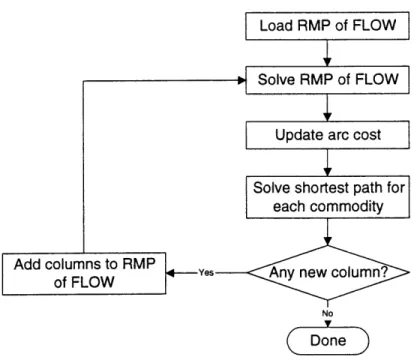
Typically, the number of blocks is large as is the number of potential block se-quences (or blocking paths) for the commodities. However, most of the blocking paths will not be used in the solution. These observations motivate the use of column generation (Barnhart, et al. [1995]) in solving the flow subproblem. The implementa-tion details of column generaimplementa-tion is summarized in Figure 2-1. Also, notice that the multicommodity flow problem becomes a set of III separable shortest path problems if there are no car volume constraints (2.36).

Block Subproblem

The block subproblem is

(BLOCK) min - (ZAk )ya (2.38)

No

Done)

Figure 2-1: Column Generation Procedure for FLOW

s.t. E ya j _ B(i), Vi E A( (2.39)

aEA

ya E {0, 1}, Va E A. (2.40)

The solution to the block subproblem will be a set of blocks that satisfy the block building capacity constraints at each node. This problem can be solved easily by simply sorting the blocks that originate at each node in non-increasing order of A' and choosing the first B(i) blocks originating at each node i. However, for any choice of Lagrangian multipliers, this solution coupled with the optimal solution of the flow subproblem will not provide a lower bound any tighter than the bound from the linear programming (LP) relaxation of the original model. This follows from the fact that the block subproblem has the integrality property, i.e., all the extreme points of the LP relaxation of BLOCK are integral. We improve the value of the lower bound by adding a set of valid inequalities to the block subproblem.

Enhanced Block Subproblem

In the block subproblem, there are no constraints imposed on the connectivity of the network. However, the blocks in any feasible solution to the original problem (BPATH) will not only meet the maximum block number constraints (2.39), they will also provide at least one origin-destination path for each commodity. The con-nectivity constraint is implied in the original path-based formulation by the forcing constraints (2.20), which were relaxed when we formed the Lagrangian relaxation. Therefore, the solution to the above block subproblem will not necessarily provide a path for each commodity. This results in a weak lower bound and causes difficulty in generating feasible solutions. To remedy this, we add the following connectivity constraints to the block subproblem.

y

y>a 1, Vcut(k) E [O(k), D(k)], Vk E IC,

aEcut(k)

where cut(k) is an element in [O(k), D(k)], the set of all possible cuts in the blocking network between the origin and destination of commodity k.

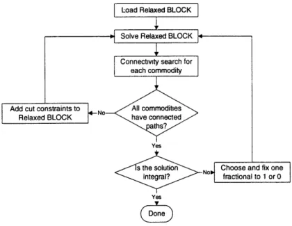
In general, there is a large number of cuts for each commodity, which is expo-nential with respect to network size. Hence, the inclusion of all these constraints is impractical, especially when the problem size is large. On the other hand, many of these constraints will be satisfied by a given solution to BLOCK. So, we use row generation, summarized in Figure 2-2, to add only the constraints that are violated by the current solution.

2.3.2

Solution Algorithms

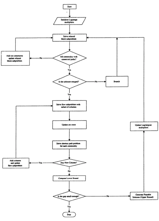
The overall solution procedure for B-PATH is summarized in the flowchart of Fig-ure 2-3. The algorithm can be divided into two parts-an Inner Loop and an Outer Loop. Given a set of Lagrangian multipliers, the two subproblems are solved sequen-tially in the inner loop, giving a lower bound to the original problem B.PATH. We also attempt to generate a feasible solution in the inner loop. Based on the solutions

Figure 2-2: Branch-and-Cut Procedure for BLOCK

to the subproblems (ft, ye), the Lagrangian multipliers are updated in the outer loop. The goal of the overall solution procedure is to search for the sharpest lower bound to the original problem (BIPATH), i.e., to solve the Lagrangian Dual (2.33). The algorithm terminates when the gap between the lower bound and feasible solution is less than a user specified tolerance.

Outer Loop

The Lagrangian Dual problem is solved by using subgradient optimization. In each iteration t, the Lagrangian multipliers are updated as follows:

kt (,t-1 + 0( Ya, (2.41)

qEQ(k)

where the notation [x]+ denotes the positive part of the vector x. To guarantee convergence (Ahuja [1993]), we choose the step size (Ot = c/t) where c is a constant and t is the iteration index to satisfy the following conditions:

lim t -+O

Yes

C±D

Figure 2-3: Lagrangian Relaxation Approach for Blocking Problem

t

limZ0, 00..

t--oo

Inner Loop

Given the Lagrangian multipliers from the outer loop, we solve the two subproblems at each iteration. The combined solutions from the two subproblems provide a valid lower bound on the optimal solution value.

Flow Subproblem

As discussed earlier, the flow subproblem is a multicommodity flow problem. Because of the exponentially large number of potential blocking paths, column generation is used to solve this subproblem. Instead of enumerating all possible blocking paths, we first solve the flow subproblem FLOW over a subset of the possible path variables. We refer to the multicommodity flow problem with only a subset of path variables as the Restricted Master Problem (RMP) of the flow subproblem FLOW. RMPs are solved repeatedly, with successive RMPs constructed by adding new path variables with negative reduced costs. The reduced cost calculations are based on the optimal solution to the current RMP. Let a and 7r be the dual variables associated with

the convexity constraints (2.35) and volume capacity constraints (2.36), respectively. Then, the reduced cost of path q can be expressed as

Cq' r = (CaVk + k k ri a) - k (2.42)

aEA iEh

The RMP solution will be optimal if Cq'" is nonnegative for all paths q E Q(k) and all commodities k; otherwise, there will exist at least one path, the addition of which might improve the RMP solution. To efficiently determine potential paths, we can solve a shortest path problem with modified arc costs (CaVk + )A + vk EiA 7r ia) for each arc a and commodity k, and compare the minimum path cost with the value of the dual variable ak.

Block Subproblem

In the enhanced block subproblem BLOCK, a set of connectivity constraints are added to make the solution to the subproblem contain at least one path for each commodity. These constraints are redundant in the original problem (B.PATH) because of the presence of the forcing constraints. However, they might be violated by solutions of the subproblem (BLOCK). Addition of these constraints will enhance the quality of the lower bound generated by the Lagrangian Relaxation. Also, as discussed later, they will improve our ability to generate feasible solutions.

Because of the large number of connectivity constraints, we use a dynamic row generation approach, called branch-and-cut, in solving this subproblem. That is, we solve it using branch-and-bound, with connectivity cuts (potentially) generated at each node of the branch-and-bound tree. We generate only the constraints that are violated by the current solution to the block subproblem and continue adding con-nectivity constraints until each commodity has at least one OD path in the BLOCK solution.

With the addition of the connectivity constraints, an integral solution is not guar-anteed in solving the LP relaxation of BLOCK. We branch on the largest fractional variables, setting them to 1, and we search the nodes of the tree in depth-first or-der. This helps to generate good feasible solutions quickly. If the original problem is feasible, we will obtain a blocking plan that contains at least one OD path for each commodity.

2.3.3

Lower Bound

Since the BLOCK and FLOW subproblems are independent, the solutions to these subproblems also solve the Lagrangian Relaxation problem £(A ). In particular, the sum of the objectives from the two subproblems provides a lower bound to the original problem B.PATH according to the Lagrangian lower bound theorem in Fisher (1981).

original problem BPATH. Due to addition of the connectivity constraints, which are implied in the original formulation (BPATH), and are valid in the Lagrangian relaxation, the Lagrangian relaxation with added connectivity constraints potentially attains a lower bound at least as large as the bound obtained by the linear program-ming relaxation of BPATH.

2.3.4

Upper Bound

Besides providing tight lower bounds, the Lagrangian relaxation approach can also generate high quality feasible solutions. Unlike existing dual-based approaches that rely on some external feasible solution generation procedure (mainly add-and-drop heuristic or branch-and-bound), Lagrangian relaxation can generate feasible solutions directly for blocking problems in which the car volume constraints are absent. A feasi-ble solution to the original profeasi-blem can be generated by solving the two subprofeasi-blems sequentially: First, the block subproblem is solved to generate a set of blocks ({ Ya})

and second, the flow subproblem is solved given the blocks selected in the first step. The solution generated is feasible if car volume constraints are not present since the blocking subproblem selects at least one OD path for each commodity.

In the general railroad blocking problem, however, the above procedure might not always find a feasible solution because the car volume constraints could be violated. We propose two methods of resolving this issue. One simple approach is to discard solutions that violate the car volume constraints. As the Lagrangian multiplier values get close to the optimal dual solution, it is more likely that the sequential procedure will find a feasible solution. This heuristic is most effective when the car volume constraints are not particularly tight. Another approach is to introduce feasibility cuts by solving a feasibility problem based on the network configuration obtained in

BLOCK:

(FEAS) min w = (2.43)

s. t. f>k6 ~ - -r k a, Vk E C,Va E A (2.44) qEQ(k) E f = 1, Vk E K: (2.45) qCQ(k) vCk k a V(i), Vi E i (2.46)

kEGK qEQ(k) aEA

f q 0, Vq E Q(k),Vk E K. (2.47)

rak > 0 Vk E 1C,Va E A (2.48)

If the optimal objective value w = 0, then the flow subproblem is feasible. Oth-erwise, at least one of the flow budget constraints is violated, forcing some flows to be sent on the arcs not selected in the solution {a} to the block subproblem. Then, a feasibility cut can be identified by the following theorem.

Proposition 2.1 When the above feasibility problem has non-zero objective (w > 0)

for a given blocking plan (ya), then, a feasibility cut of the form Zae ya > 1 can be

identified if the problem is feasible, where F is a set of blocks not selected in the block subproblem (that is, Va = 0) with associated positive dual values.

Proof Suppose that (-01), Uk, and (-7rs) are the duals associated with constraints 2.44, 2.45 and 2.46, respectively. The dual of the above feasibility problem is:

(DUALFEAS) maxzdual = E

>3

3

3

aEA kEK: kEKC iECJ

s.t.

-3 6

+

ak

-<-

Vq e

Q(k), Vk

e

K:

(2.50)

aEA iENr aEA

Ok < 1 Va E A, Vk E (2.51)

, w7ri 0, Vi E Kn, Va E A, Vk E K. (2.52)

We can interpret the O 's as commodity specific non-negative tolls associated with using block a and w7r as non-commodity specific non-negative tolls associated with