Limits of slow sound propagation and transparency in lossy, locally resonant periodic structures Limits of slow sound propagation and transparency in lossy, locally resonant periodic structures

HAL Id: hal-02406563

https://hal.archives-ouvertes.fr/hal-02406563

HAL is a multi-disciplinary open access archive for the deposit and dissemination of sci-entific research documents, whether they are pub-lished or not. The documents may come from teaching and research institutions in France or abroad, or from public or private research centers.

L’archive ouverte pluridisciplinaire HAL, est destinée au dépôt et à la diffusion de documents scientifiques de niveau recherche, publiés ou non, émanant des établissements d’enseignement et de recherche français ou étrangers, des laboratoires publics ou privés.

lossy, locally resonant periodic structures Limits of slow

sound propagation and transparency in lossy, locally

resonant periodic structures

Georgios Theocharis, Olivier Richoux, V Romero García, Aurélien Merkel, V.

Tournat

To cite this version:

Georgios Theocharis, Olivier Richoux, V Romero García, Aurélien Merkel, V. Tournat. Limits of slow sound propagation and transparency in lossy, locally resonant periodic structures Limits of slow sound propagation and transparency in lossy, locally resonant periodic structures. New Journal of Physics, Institute of Physics: Open Access Journals, 2014, 16, �10.1088/1367-2630/16/9/093017�. �hal-02406563�

This content has been downloaded from IOPscience. Please scroll down to see the full text.

Download details:

IP Address: 195.221.243.134

This content was downloaded on 12/11/2014 at 08:34

Please note that terms and conditions apply.

Limits of slow sound propagation and transparency in lossy, locally resonant periodic structures

lossy, locally resonant periodic structures

G Theocharis, O Richoux, V Romero García, A Merkel and V Tournat

LUNAM Université, Université du Maine, CNRS, LAUM UMR 6613, Avenue O. Messiaen, 72085 Le Mans, France

E-mail:georgiostheocharis@gmail.com

Received 15 May 2014, revised 7 July 2014 Accepted for publication 24 July 2014 Published 15 September 2014

New Journal of Physics 16 (2014) 093017 doi:10.1088/1367-2630/16/9/093017 Abstract

We investigate sound propagation in lossy, locally resonant periodic structures by studying an air-filled tube periodically loaded with Helmholtz resonators and taking into account the intrinsic viscothermal losses. In particular, by tuning the resonator with the Bragg gap in this prototypical locally resonant structure, we study the limits and various characteristics of slow sound propagation. While in the lossless case the overlapping of the gaps results in slow-sound-induced transparency of a narrow frequency band surrounded by a strong and broadband gap, the inclusion of the unavoidable losses imposes limits to the slowdown factor and the maximum transmission. Experiments, theory, and finite element simulations have been used for the characterization of acoustic wave propaga-tion by tuning the Helmholtz/Bragg frequencies and the total amount of loss both for infinite and finite lattices. This study contributes to the field of locally resonant acoustic metamaterials and slow sound applications.

Keywords: slow sound, acoustic metamaterials, lossy periodic structures

1. Introduction

Locally resonant periodic structures exhibit two types of band gaps in their dispersion relation: the resonator and Bragg gaps. These stem from the two available interference mechanisms in this kind of structure: the Fano-type and the Bragg-type constructive interference of reflections.

Content from this work may be used under the terms of theCreative Commons Attribution 3.0 licence. Any further distribution of this work must maintain attribution to the author(s) and the title of the work, journal citation and DOI.

The configuration at which these two gaps are tuned to each other and overlap is particularly interesting (see [1] for an example in acoustics and [2] in optics). In the case of the exact overlap, the lossless theory predicts a strong and broadband gap. This phenomenon has been studied in different branches of physics, including elastic waves [3], split-ring microwave propagation [4], and duct acoustics [5], among others. It is even more interesting when these two different types of gaps do not exactly overlap, but are detuned to be very close to each other. In this case, ignoring again the losses, the theory predicts an almost-flat propagating band which is very attractive for slow wave applications.

In acoustic waveguides, these configurations were first studied by Sugimoto [5] and Bradley [6]. In recent years, they have reignited interest due to their importance in sound isolation [7,8] and slow sound propagation [9,10]. However, in these studies, there is either no systematic characterization of the slow sound propagation [5, 6] or the role of losses is underestimated [9, 10]. The latter could lead to misleading conclusions because, as has been shown in relevant works [11–14], flat propagating bands corresponding to slow wave propagation acquire an enhanced damping when compared to bands with larger group velocities. Thus, in the case of slightly detuned gaps (i.e., once the Bragg and resonator gaps are slightly different), the presence of losses could totally destroy the almost-flat band that the lossless case predicts. The aim of this work is to fill this gap by studying in detail the slow sound propagation in periodic locally resonant structures while considering loss and finite-size effects. For that reason, we chose a prototypical locally resonant acoustic structure—a tube periodically loaded with Helmholtz resonators (HRs)—considering the viscothermal losses [15] imposed by the waveguide and resonator boundary walls.

Our study contributes to the field of locally resonant acoustic metamaterials [16] which derive their unique properties, such as negative effective mass density [17] and negative bulk modulus [18,19], from local resonators contained within each unit cell of engineered structures. Due to these effective parameters, a plethora of fascinating phenomena have been proposed in recent years, including negative refraction, super-absorbing sound materials, acoustic focusing, and cloaking (see [20] and references therein). Although the inclusion of losses in locally resonant structures is very important, their role in some studies has been totally ignored. Loss is not only an unavoidable feature, but it may also have deleterious consequences on some of the novel features of metamaterials [21], including double negativity and cloaking.

In addition, this work contributes to other applications of the field of slow sound, such as acoustic transparency [10, 22–25] and the acoustic rainbow effect [26]—fields that have experienced an increase in interest recently, following the trend in their optical and plasmonic counterparts (see, for example, [27, 28] for slow light in optical structures and [29] for rainbow trapping effects in plasmonics). In optics, the study of slow light phenomena has increased due to potential applications in areas such as signal processing, sensing, and enhanced nonlinear effects (see [27, 28] and references therein). In acoustics, slow sound propagation is relevant to the design of narrow-band transmission filters, delay lines, and switches. Moreover, slow sound propagation opens perspectives in ways to enhance nonlinear effects at local resonances [30]. This is of great importance and could increase the functionality of acoustic metamaterials, leading to novel nonlinear acoustic devices for sound control at low frequencies.

In this paper, after presenting the theory and the experimental setup, we continue with results and discussion. In particular, (i) we experimentally and theoretically study the coupling of Bragg and resonator band gaps, (ii) we present the limits of slowness at the band edges, imposed by losses in the waveguide and in the resonators, (iii) we describe and calculate

important features of slow, dispersion-free sound propagation, and (iv) we explore the finite-size effects in lossy structures. Finally, we present our conclusions.

2. Theory

The propagation of linear, time-harmonic acoustic waves in a waveguide periodically loaded by side branches was first studied in [6]. Using Bloch theory and the transfer matrix method, one can derive the following dispersion relation (see also [5, 31]):

= + qL kL j Z Z kL cos ( ) cos ( ) 2 sin ( ), (1) c b

where q is the Bloch wave number, k is the wave number in air, L the lattice constant, Zbthe

input impedance of the branch (see [31] for the case of HR branch), and Zc= ρ0 0c S is the

characteristic acoustic impedance of the waveguide where S is its cross-sectional area.ρ c₀, 0 are

the density and the speed of sound in the air, respectively, and j = −1 . The dispersion relation exhibits two types of band gaps: the resonator gap and the Bragg gap. These band gaps stem from the two different reflection mechanisms in periodic structures with side branches. The first is related to Fano resonances/interference while the latter comes from Bragg-type constructive interference of reflections.

The transmission coefficient through a finite lattice can be derived using the transmission matrix method. For the case of N side branches, the total transmission matrix can be expressed as follows [8, 22, 32]: ⎛ ⎝ ⎜_UP ⎞_⎠⎟=

(

)

represent the transmission matrices for the propagation through a length, L, in the waveguide and through a resonant branch, respectively. Pin (Uin) and Pout (Uout) are the pressure (and

respective volume velocity) at the input and output of the structure. Considering the previous equations, the pressure complex transmission and reflection coefficients can then be calculated [8] as = + + + t T T Z T Z T 2 , (5) 11 12 0 21 0 22 = +₊ −₊ −₊ r T T Z T Z T T T Z T Z T . (6) 11 12 0 21 0 22 11 12 0 21 0 22

The sound waves are always subjected to viscothermal losses on the wall. Viscothermal losses are taken into account by considering a complex expression for the wave number. In our case, we used the model of losses from [15]; namely, we replace the wave number and the impedances by the expressions

⎜ ⎟ ⎛ ⎝ ⎞⎠ ω β _{γ χ} = + + − k c0 1 s(1 ( 1) ) , (7) ⎜ ⎟ ⎛ ⎝ ⎞⎠ ρ _β γ χ = + − − Z c S 1 s (1 ( 1) ) , (8) 0 0

by settings = Ri δ where Riis the radius of the considered tube (i = t for the waveguide, i = n

for the neck, and i = c for the cavity of the HRs) and_{δ =} μ

ρ ω

2

0 is the viscous boundary layer

thickness, with μ being the viscosity of air. χ = Pr with Pr, the Prandtl number at atmospheric

pressure; and β = (1 − j) 2 andγ = 1.4, the heat capacity ratio of air.

3. Experimental setup

The experimental setup, sketched in figure1, is composed of an impedance sensor within which there are two microphones and a piezoelectric source (see appendix A), the sample (a cylindrical tube, side loaded with HRs), a third microphone after the last loaded HR (BK 4136 microphone, carefully calibrated), and a termination end which can be considered as anechoic (see appendixCfor further details). The sample is composed of a cylindrical waveguide with an inner radius, Rt= 2.5 cm, and a wall thickness of 0.5 cm. Its characteristic impedance is Zc. The

first cutoff frequency of nonplanar acoustic propagation in the waveguide is around 4 kHz, which is well above the highest frequency of measurement, 1 kHz. Thus, only plane waves can propagate, and the propagation can be considered one-dimensional. The HRs are side loaded to the waveguide and composed of a cylindrical neck, with an inner radius, Rn = 1 cm, and a

length, ln = 2 cm, and a cylindrical cavity with an inner radius, Rc = 2.15 cm, and a variable

length, lc. The length correction of the neck due to radiation was experimentally measured at

1.04 cm by comparing the input impedances (experimentally and theoretically) for different volumes of the HR cavity. This is in very good agreement with the theory (see appendixB).

The distance between two consecutive resonators is L = 30 cm, which is therefore the length of a unit cell. Considering the termination as anechoic, we assume thatP U3 3₌ Zcat the position

of the third microphone. To calculate the transmission matrix of one cell, we take into account the reciprocity and symmetry of one cell. To satisfy the symmetry condition, we consider the pressure, P˜out, at the position x˜out, which is located at L 2 after the last resonator, and we

calculate the impedance,Z˜ ₌ P U˜in ˜in, at the position x˜in, which is located atL 2 = 15 cm before

the first resonator. This is calculated by transferring the measured input impedance,Z = P Uin in,

at the position x˜in. From Z˜ and H˜inout = P˜out P˜in, the transfer Mcellmatrix of a cell is then found;

that is, ⎛ ⎝ ⎜⎜P ⎞_⎠⎟⎟ = ⎛_⎝⎜⎜ ⎞_⎠⎟⎟ =

( )

The Bloch wavenumber, q, and the dispersion relation can be found using

= +

q acos[(A D) 2] (ncellL) [33, 34], where ncell is the number of cells. The exact shape of

the dispersion curve is obtained by phase unwrapping and by restoring the phase origin [34].

4. Results and discussion

4.1. Coupling of the Bragg and resonator gaps

We start by studying the coupling between the Bragg and resonator gaps, taking into account viscothermal losses. In figure2(a)–(d), one can see both the experimental (red solid line) and theoretical (black dashed line) complex dispersion relations for two different resonance frequencies of the HRs, in comparison with the theoretical lossless case (green dotted line). For the fixed lattice distance of L = 30 cm, the first Bragg resonance appears atk LB = π, and thus at

= ≈

f_{B 2}c_L0 571_{Hz. The resonance frequency, f}

0, of the HRs is in general unknown. One can use

the traditional lumped-parameter model [32] to obtain an analytical expression. However, this is valid only at very small frequencies and it requires the exact knowledge of the length corrections. Therefore, we tune the resonant frequency with the Bragg frequency by experimentally calculating the dependence of the imaginary part of the complex dispersion relation on the length of the cavity, lc, of the HR (see figure2(e)). We define a detuning length

parameter, Δ = −l lc l0, where l0corresponds to the cavity length at which f0 = fB. Thus, Δl

measures how far we are from the complete overlap between the Bragg and HR resonances. As shown in figure2(e), if Δ <l 0 (Δ >l 0), the HR resonance approaches the Braggʼs resonance from higher (lower) frequencies. According to [5], for the special case of Δ =l 0, a wide band gap appears in the region f_B(1 − ( 2) )κ 1 2 < <f f_B(1 + ( 2) )κ 1 2 _{, where κ =} S l

SL

c c _(with

π

=

Sc Rc2) measures the smallness of the cavityʼs volume relative to the unit cellʼs volume.

For our case, the above expression predicts a band gap of416.5 < <f 727.7 Hz, which is in very good agreement with the experiments. In practice, though, it is very difficult to find the case of_{Δ =}l 0 because one needs to control either the length of the cavity or the lattice constant with high precision. When _{Δ ≃}l 0, as seen in figures 2(a) and (b), one can observe that the lossless theory (green dotted line in figure 2(a)) predicts an almost-flat branch inside the band gap. As we mentioned before, this is of particular interest for slow sound propagation.

However, this branch is drastically reduced once losses are introduced. In contrast, for

Δ =l 0.4 cm (figures2(c) and (d)) the branch inside the band gap is more robust to losses. Thus, we conclude that the slowness of sound propagation depends crucially on the detuning parameter, _{Δl, but the intrinsic losses impose a limit on it.}

4.2. Limits of slow sound

In periodic structures, the group velocity vanishes at the band gap edges. However, the inclusion of losses results in the group velocity acquiring a finite value above zero [11]. In this section, we study the limits of slow sound at the band edges, originating both from Bragg and resonant reflections, due to lossy HRs and/or lossy waveguides. We introduce the group index as a slowdown factor from the speed of sound, c, defined asng ≡ c υg where υ =g (_{∂Re q}∂ω_{( )})is

the group velocity. In lossy periodic structures, the real and imaginary parts of the group velocity correspond to propagation velocity and pulse reshaping, respectively (see [12] and references within). Negative values of ngcorrespond to negative group velocity induced by the

losses. This implies no loss of causality, but is rather due to strong reshaping of the pulse [35]. In figure 3, we present the group index for a periodic structure with Δ =l 0.4 cm. In the absence of losses (solid lines in figures3(a) and (c)), one can see the singularities near the band gap edges, which result in a vanishing group velocity. The first singularity (lower frequency peak) is connected with the resonator gap while the second with the Bragg gap (higher frequency peak). However, this picture changes considering the losses. In locally periodic structures, there are two kinds of losses: (a) distributed, through the propagation at the waveguide, and (b) lumped, which occur only at the discrete locations of the lossy resonators.

Figure 2. (a)–(d) Representation of the complex dispersion relation for the case of

Δ ≃l 0 cm (a)–(b), and Δ =l 0.4 cm (c)–(d). Black dashed line shows the analytical lossy case. Green dotted line represents the analytical lossless case. Red solid line shows the experimental result. (e) Experimental values of Im(qL) as a function of the detuning parameter, Δl.

In figure3(a), we present the group index of the structure taking into account only the lumped losses due to the HRs and in figure 3(c), considering only distributed propagation losses. The conclusion is that the first maximum of the group index is mostly affected in the losses in the HRs, while the second maximum in the losses in the waveguide. Here, we have to mention that the tuning of the losses in experiments can be obtained by different ways, see equation (8). For example, by using different media to fill in the structure (air, water, etc), by changing the environmental conditions (for example the temperature), or by changing the geometrical characteristics of the sample (radius of the tube, radius and length of the neck of the HRs, volume cavity of the HRs). By changing only the geometrical characteristics of the HRs, one can tune the resonator losses, keeping the same propagation losses.

Figure 3.(a) Group index as a function of frequency for a lossless waveguide and lossy resonators with Q0 ₌836 (dashed line) and Q0= 83 (dotted line). Solid line

corresponds to the lossless case. (b) Maximum of group index around the lower edge as a function of the Q0of the HRs. (c) Group index as a function of frequency for the

case of lossless resonators and lossy waveguide with a loss factor of 0.0015 (dashed line) and 0.0152 per unit length. (d) Maximum of group index around the upper edge as a function of the losses per unit length. All the cases correspond to Δ =l 0.4 cm.

In figure 3(b), we plot the maximum of the group index around the lower band edge (due to the resonators) as a function of the quality factor Q0, of the resonators, considering a lossless

waveguide. Increasing the losses into the HRs (decreasing the Q0) the maximum group index

around this edge decreases. The Q0 of the HRs was calculated as [32]:

ω =

_{( )}

where M is the mass of the air in the neck of the HRs (taking into account also the length corrections) andRe ( )Zb is the real part of the branch impedance that describes the losses of the

HRs due to viscothermal losses on the wall of both the neck and the cavity. In figure3(d), we consider lossless HRs and we plot the maximum of the group index around the upper band edge (due to the Bragg reflection) as a function of a loss factor that characterizes the loss per unit length through the propagation in the waveguide. This factor is defined as the absolute value of the imaginary part of the wavenumber, given by equation (7), at the frequency of the maximum group index. The presence of the losses into the waveguide (viscothermal losses at the wall of the waveguide) puts a limit on the maximum slowness due to periodicity.

In figure 4(a), we show the theoretical (black dashed line) and experimental (orange solid line) group index for the case of Δ =l 0.8 cm, considering the whole amount of viscothermal losses in both the waveguide and resonators that the theory (see equations (7)–(8)) predicts. We considered the sample to be filled with air, at atmospheric pressure and temperature of 20 °C. There is very good agreement between our lossy theory and the experimental results. The disagreement around the first maximum of the group index could be explained by imperfections in the geometrical characteristics of the HRs and underestimation of the resonator losses. In figure 4(b), we show the experimental group index for different values of the detuning

Figure 4.(a) Experimental (orange line) and theoretical (black solid line) group index with _{Δ =}l 0.8 cm. (b) Experimental group index as a function of the detuning parameter, _Δl.

parameter, Δl. The maximum group index always appears around the lower band edge, indicating that in our locally resonant acoustic structure, the slowest sound propagation appears near the edge of the resonator gap.

4.3. Slow, dispersion-free sound propagation

In the previous section, we focused on the minimum value of group velocity (maximum value of slowness), which appears at the band edges. However, in slow wave propagation, there are two additional important properties that need to be characterized. The first one is the frequency bandwidth of the phenomenon, which needs to be as wide as possible but this comes with the price of small group index. The second one is the effect of higher-order dispersion. Configurations like the one in [25] lead to narrow-band transmission and strong dispersion. Here, we focus on configurations where both the group index is high enough and the dispersion-induced pulse distortion is at a minimum. The distortion of the pulse can be analyzed by means of the group velocity dispersion (GVD)1, which needs to be at a minimum to produce low distortion. In optics, the higher-order dispersion can be suppressed by periodic coupled resonator structures such as coupled-resonator optical waveguides (CROWs) and side-coupled integrated sequence of spaced optical resonators (SCISSORs) (see, for example, [27]). The structure we analyze here can be considered an acoustical analog of the SCISSORs. A more useful regime for slow sound propagation is not around the band edges, but around the flat intermediate band that results when the Bragg and resonator gaps are tuned close to each other. This is because this intermediate regime can support small group velocities and, at the same time, a very small GVD. In particular, the GVD becomes zero at a frequency between the two band edges, where the group index takes the minimum value. To avoid the higher dispersion distortion, the propagating pulse should be centered around this frequency, while its usable bandwidth for a dispersion-free and slow pulse propagation can be defined as half of the bandwidth between the two maxima.

In figure5(a), we plot the group index for three different values of the detuning parameter,

Δl, considering two different lossy cases: a weak lossy case (dashed line) and the lossy case that

corresponds to the experimental conditions. As one can see, the bandwidth and the value of the group index where GVD is zero depend crucially on the detuning parameter,Δl. Comparing the two lossy cases, one can conclude that the value of the group index where GVD is zero is influenced by the total amount of losses only whenΔ →l 0. In figure5(b), we plot the value of the group index where GVD is zero and in figure 5(c), we plot the usable bandwidth as a function ofΔl for the lossy, experimentally relevant case. As Δl increases, the usable bandwidth increases, but at the same time the group index significantly decreases. For large enough values of the detuning parameter, _{Δl, the group velocity of the sound pulse approaches the speed of} sound. Experiments (circles) are in good agreement with lossy theory.

1 _{Once the group velocity depends on frequency in a medium, one can introduce the Group Velocity Dispersion}

(GVD), GVD =_{∂ ∂}2k _ω2_{. This parameter is for example used in optics for the analysis of the dispersive temporal}

4.4. Finite lossy structures

Up to now, we have studied the basic properties of slow sound propagation in infinite periodic structures. In reality, however, systems are finite. In this section, we address the finite-size effects.

As is known, the transmission spectrum in finite size structures is not flat, but has ripples. The peaks correspond to Fabry–Perot-like modes, and they can cause distortion to a propagating pulse and limit the bandwidths of the device. For the case of acoustic pulse propagation in finite, locally resonant periodic structures with HRs, one can refer to [25]. In that study, the authors consider the slow sound propagation of a narrow-band signal in a finite periodic structure composed of four detuned HRs. The signal at the end of the structure seems not to be distorted much by finite-size effects. We believe that this is because of the presence of losses which, as we show in this section, can smooth the transmission amplitude of the peaks, creating a broadband of the transmitted frequencies with similar values of the transmission coefficient. In the next part of this section, we focus on another very interesting study, which is the effect of losses on the transmission peaks that correspond to slow sound modes. In particular, we investigate the connection between the slowness (inverse bandwidth) of the modes and the effect of resonator losses. We start our analysis with a lossless, locally resonant structure composed of N HRs. Numerical simulations using the finite element method (FEM) have been

Figure 5.(a) Group index for three different values of Δ =l 0.2, 0.8, 1.4 cm. The loss per unit length within the waveguide is around 0.003 (dashed line) and 0.03 (solid line), while the quality factor of the HRs is aroundQ0 ₌800(dashed line) andQ0 =80(solid

line). (b) The value of the group index at the frequency where the GVD is zero as a function of the detuning parameter,_{Δl. (c) The bandwidth, defined as half the frequency} regime between the two maxima as a function of _{Δl. In both (b) and (c), the solid line} corresponds to the fully lossy theory, while circles correspond to experiments.

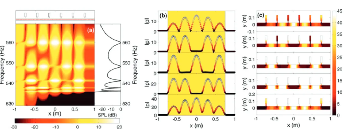
performed to highlight the transmission and field distribution inside the waveguide loaded with N = 6 HRs for the case ofΔ =l 0.8 cm. A plane wave, traveling from left to right, is considered. The ends of the tube in the numerical domain are surrounded by perfectly matched layers in order to numerically approximate the Sommerfeld radiation condition. Figure 6(a) shows frequency-position maps of the sound pressure level (SPL) for the frequency range of 530–570 Hz. This frequency range is around the propagating band, which is formed by the detuning of the Bragg and resonator gaps. Due to the finite length of the structure, instead of a continuous propagating band, one can observe the presence of peaks in the transmission spectrum (see the right part of figure6(a)) that correspond to transparency resonances. For the case of N = 6 resonators, there are N − =1 5 discrete transmission peaks with unity transmission (T= | |t 2 = 0 _{dB)). In general, the stronger the dispersion is, the narrower the} bandwidth of the modes. Consequently, because dispersion is stronger at the edges than in the rest of the propagating band, transparent modes close to the edges exhibit narrower bandwidth compared to the others. For the case of N = 6 and _{Δ =}l 0.8 cm, as shown in the inset of figure 6(a), the higher transparent modes (at 548, 560 Hz) are not located close enough to the upper edge to exhibit narrow bandwidth, while the lower modes (at 536, 538 Hz—close enough to the lower edge) are characterized by a very small bandwidth (ultra-slow sound transparent modes).

In figures6(b) and (c), one can see the profiles of these transparent modes along the axis of propagation, as well as their complete distribution of the sound pressure level. The profile of the first mode at 536 Hz is similar to the profile of the fifth mode at 560 Hz. Also, the profile of the second mode at 538 Hz is similar to the fourth mode at 548 Hz. The amplitude of these modes is inversely analog to their bandwidth. Thus, the first transparent mode, which is characterized by a very small bandwidth, is also characterized by a large pressure amplitude. Looking at the complete sound pressure level (figure6(c)), one can also see the role of the HRs in these modes. Thus, the HRs are highly excited for the first three transparent modes, and not so much for the last two. Although in the lossless case at these resonant frequencies there is total transmission,

Figure 6.(a) Numerical sound pressure level,20 log (| |), obtained using FEM, for thep

range of frequencies between 530 Hz and 570 Hz inside the tube loaded with six HRs along the line shown in the upper insets (red dashed line) for the lossless case with

Δ =l 0.8 cm. Right inset shows the frequency dependence of the sound pressure level at the end of the structure. (b) Profiles and (c) complete distribution of sound pressure levels for the five peaks shown in (a). From top to bottom in (b) and (c): 560 Hz, 548 Hz, 541 Hz, 538 Hz, and 536 Hz.

in the presence of losses the behavior is dramatically modified. In order to compare with the lossless case, we start the analysis by considering only the lumped resonator losses. Namely, we study the case where the propagation into the waveguide is lossless, while the side-loaded resonators are lossy. Then, we increase the losses in the resonators (decrease their quality factor, Q0) and we look at the transmission (T = | |t 2) and absorption (A = −1 | |t 2− | |r 2) as a

function of the frequency, as shown in figure7. The presence of the viscothermal losses into the HRs results in a significant degradation of the transmission (see the left panels of figure 7). Ultra-slow sound transparent modes, located very close to the edges and characterized by very small bandwidth, disappear even with the inclusion of weak losses. For an example, see figure 7(b), where the transmission through a structure with very weakly lossy resonators (quality factor of HRs around 8000) is presented. On the other hand, transparent modes with a moderate bandwidth are more robust to losses, as, for example, the fourth and fifth resonant modes, as seen in figure7(a).

In order to answer the question of what happens to the energy that is not transmitted around the transparent modes, we also plot the absorption as a function of the frequency, increasing the losses in the HRs (decreasing the Q0), as shown in figures 7(c) and (d). For a

given value of Q0, one can see that the absorption coefficient is different for each transparent

mode. For high values of Q0(low HR losses, see figure7(d)), the small bandwidth modes (ultra

slow sound transparent modes) show larger absorption compared to the others. In general,

Figure 7.(a), (b) Transmission as a function of the frequency and the quality factor of HRs, Q0. (c), (d) Absorption as a function of the frequency and the Q0. All the diagrams

are for a lattice of six HRs loaded in a lossless waveguide, with_{Δ =}l 0.8 cm. Panels (b) and (d) correspond to high values of Q0and they are plotted in linear scale, while panels

increasing the losses in the HRs, the absorption coefficient for each transparent mode reaches a maximum value of 0.5–0.6 and then decreases. The value of Q0at which the absorption reaches

its maximum value is different for each transparent mode. This can be explained by taking into account the interplay of the bandwidth of each mode (which depends on the coupling between the resonator and the waveguide) and the energy decay rate due to the lumped losses (lossy resonators) [2].

Up to now, we have studied the case of Δ =l 0.8 cm. However, as we showed, the dispersion, and thus the bandwidth of the modes, depends crucially on the detuning parameter,

Δl. Therefore, we study in more detail the role of the detuning parameter, Δl in finite structures.

We consider the total amount of viscothermal losses (both distributed and lumped) for the experimentally relevant conditions: air-filled structure, atmospheric pressure, and temperature of 20 °C. From systematic studies, we found that the above-mentioned phenomenology regarding the transmission and absorption coefficients does not qualitatively change with the inclusion of distributed losses. In figure8, we plot the transmission, reflection, and absorption coefficient for the case of six HRs with (a)Δ =l 0.2 cm, (b) _{Δ =}l 0.8 cm, and (c) _{Δ =}l 1.4 cm. For very small values of the detuning (for example, _{Δ =}l 0.2 cm), we see that almost all the energy is reflected. In this case, the lossless theory gives five ultra-slow sound transparent modes. All these transparent modes disappear due to losses. For larger values of_{Δl, part of the} energy is reflected and part is absorbed. In particular, for Δ =l 0.8 cm, only two peaks are evident in the transmission diagram, and three in the absorption diagram. The first two transparent resonances, which are characterized by a very small bandwidth, disappear and the energy around these two frequencies is mostly reflected. In conclusion, the acoustic response of the structure around the propagating band formed from the detuning of the Bragg and resonator gaps depends crucially on the presence of losses—mostly the losses in the resonators—and the detuning parameter,Δl. For a very small detuning, with Δl close to 0, the finite structure leads to ultra-slow sound resonant modes and the losses have a deleterious effect, leading to reflection of the acoustic energy around these frequencies.

Figure 8. Transmission, reflection, and absorption of a periodic structure of six HRs with (a) _{Δ =}l 0.2 cm, (b) _{Δ =}l 0.8 cm, and (c) Δ =l 1.4 cm, taking into account all viscothermal losses.

5. Conclusions

In conclusion, we have studied slow sound propagation in locally resonant acoustic structures, taking into account the inevitable existence of viscothermal losses and finite-size effects. First, we characterized experimentally the dispersion relation of a structure, where we tuned the two kinds of band gaps that these structures exhibit. Perfect agreement was found by direct comparison with lossy theory. Second, we investigated the maximum slowness of the sound propagation, which happens at the edges of the propagating band, considering the cases of lossy HR-lossless waveguides and lossless HR-lossy waveguides. Losses are responsible for the existence of a maximum value of slowness; the theoretically predicted near-zero group velocity disappears due to losses. Then, we characterized two important features of the slow sound pulse propagation: the dispersion-free propagation and its relevant bandwidth. A trade-off among the relevant parameters (group index, bandwidth, and detuning) has been presented. Finally, we considered the finite-size effects. A detailed analysis revealed that the acoustic response of locally resonant periodic structures around the propagating band, formed from the detuning of the Bragg and the resonator gaps, depends crucially on the presence of losses—mostly the losses in the resonators—and the detuning parameter, _Δl.

The idea of slow sound propagation can be extended in quasi two-dimensional structures [36], two-dimensional resonant sonic crystals [1, 37], and three-dimensional arrays of resonant spheres [38] by coupling the Bragg and the resonator band gaps. This could result in some interesting phenomena like slow sound filtering, broadband attenuation, and the enhancement of nonlinear processes in two- and three-dimensional structures. We believe that this experimental and theoretical study shows the great importance of losses in acoustic wave propagation through periodic locally resonant structures, and it contributes to very promising research in the field of acoustic metamaterials and slow wave applications.

Acknowledgments

We acknowledge V Pagneux, J P Dalmont, and A Maurel for useful discussions. This work has been funded by the Metaudible project ANR-13-BS09-0003, co-funded by ANR and FRAE. G T acknowledges financial support from the FP7-People-2013-CIG grant, Project 618322

ComGranSol. VRG acknowledges financial support from the ‘Pays-de-la-Loire’ through the post-doctoral program.

Appendix A. Impedance sensor

The impedance sensor [39] has been developed jointly by CTTM2 and LAUM3. The input impedance of the tested tube, Z = P Uin in, at the position xin is measured with a precision of

±1% in amplitude, ± °0.5 in phase, and ±0.5% in frequency. The impedance sensor is composed of a closed-back cylindrical cavity separated by a piezoelectric buzzer, which is the acoustic source to an opened, front cylindrical cavity. As shown in figureA.1, the lengths L1

and L2are the lengths of the back cavity and the front cavity, respectively. The lengths L1″and

″

L2 are the distances between the microphone 1 and the back wall of the sensor and between the

microphone 2 and the reference plane, respectively. D1andD2are the diameters of the back and

front cavities, respectively. From the diameters, the characteristic impedances of the cavities,

ZIS

1 for the back cavity, andZ2IS for the front cavity are derived using equation (8). Microphone

1 measures the pressure in the back cavity PIS

1 . Microphone 2 measures the acoustic pressure in

the front cavity P₂IS.

The input impedance at the reference plane Z is derived from [40]

= − − Z H B K H C (A.1) 12 12

with the transfer function H = P sIS (P sIS )

12 2 2 1 1 , where s1 and s2 are the sensitivities of

microphones 1 and 2, B = iZIS tan (kL″)

2 2 , C= itan (kL2) Z2IS, and K depends on the

dimensions of the sensor and the sensitivities of the microphones. K is determined through a calibration measurement using a rigid wall at the reference plane. Thus, considering that

→ ∞

Z , H₁₂cal = K C. A third carefully calibrated microphone is placed close to the anechoic termination of the setup in order to measure the acoustic pressure P3 and to determine the

transfer matrix from the transfer function, H13 = P P3 1IS.

Appendix B. Length corrections of the HRs

The correction on the lengthlcorr_{of the neck is deduced from the sum of two correction lengths,}

= +

lcorr l l

1corr 2corr, which are estimated using the two following expressions:

⎡ ⎣ ⎤⎦ = − +

(

)

(

)

(

)

(

)

The correction given by equation (B.1) is due to the discontinuity from the neck to the cavity of the Helmholtz resonator [41]. The correction given by equation (B.2) is due to the discontinuity from the neck to the principal waveguide [40]. From equations (B.1) and (B.2), the correction 2 _{Centre de Transfert de Technologie du Mans, 20, rue Thalès de Milet, 72000 Le Mans, France}

length is lcorr = 0.96 _{cm. Experimentally, we calculated l}corr _{= 1.04 cm. The disagreement}

between theory and experiments is less than 8%and it could be explained by imperfections in the geometry of the HRs.

Appendix C. End termination

The end termination is a structure composed of a purely resistive metal tissue and a tunable coupling adaptor (discontinuity of section) [42]. By calculating the reflection coefficient of the tube without the HRs, (as seen in figureC.1) we found that this is below 5% for the frequency range of 100–900 Hz. Thus, we consider this structure as an anechoic termination for our further analysis.

References

[1] Croënne C, Lee E J S, Hu H and Page J H 2011 AIP Adv.1 041401

[2] Xu Y, Li Y, Lee R K and Yariv A 2000 Phys. Rev. E62 7389

[3] Xiao Y, Mace B R, Wen J and Wen X 2011 Phys. Lett. A375 1485

[4] Kaina N, Fink M and Lerosey G 2013 Sci. Rep.3 3240

[5] Sugimoto N and Horioka T 1995 J. Acoust. Soc. Am.97 1446

[6] Bradley C E 1994 J. Acoust. Soc. Am.96 1844

[7] Weng X and Mak C 2011 J. Acoust. Soc. Am.131 1172

[8] Seo S-H and Kim Y-H 2005 J. Acoust. Soc. Am. 118 2332

[9] el Boudouti E H et al 2008 J. Phys. Condens.: Matter20 255212

[10] Yu G and Wang X 2014 J. Appl. Phys.115 044913

[11] Pedersen J G, Xiao S and Mortensen N A 2008 Phys. Rev. B78 153101

[12] Chen P Y et al 2010 Phys. Rev. A82 053825

[13] Moiseyenko R P and Laude V 2011 Phys. Rev. B83 064301

[14] Andreassen E and Jensen J S 2013 J. Sound. Vib.135 041015

[15] Zwikker C and Kosten C W 1949 Sound Absorbing Materials (Amsterdam: Elsevier) [16] Lu M-H, Feng L and Chen Y-F 2009 Mater. Today12 34

[17] Zhengyou L, Xixiang Z, Yiwei M, Zhu Y Y, Zhiyu Y, Chan C T and Ping S 2000 Science289 1734

[18] Fang N, Xi D J, Xu J Y, Ambati M, Srituravanich W, Sun C and Zhang X 2006 Nat. Mater.5 452

[19] Lee et al 2012 Phys. Rev. B86 184302

[20] Deymier P A 2013 Acoustic Metamaterials and Phononic Crystals (Heidelberg: Springer)

Craster R V and Guenneau S 2013 Acoustic Metamaterials: Negative Refraction, Imaging, Lensing and Cloaking (Heidelberg: Springer)

[21] Solymar L and Shamonina E 2009 Waves in Metamaterials (New York: Oxford University Press) [22] Santillán A and Bozhevolnyi S I 2011 Phys. Rev. B84 064304

[23] Sánchez-Dehesa J, Torrent D and Cai L W 2009 New J. Phys.11 013039

[24] Liu F et al 2010 Phys. Rev. E82 026601

[25] Santillán A and Bozhevolnyi S I 2014 Phys. Rev. B89 184301

[26] Zhu J et al 2013 Sci. Rep.3 1

Romero-García V, Picó R, Cebrecos A, Sánchez-Morcillo V J and Staliunas K 2013 Appl. Phys. Lett.102 091906

[27] Khurgin J B and Tucker R S 2009 Slow Light: Science and Applications (Boca Raton, FL: CRC Press) [28] Baba T 2008 Nature Photon.2 465

[29] Tsakmakidis K L, Boardman A D and Hess O 2007 Nature450 397401

Jang M S and Atwater H 2011 Phys. Rev. Lett.107 207401

[30] Richoux O, Tournat V and le van Suu T 2007 Phys. Rev. E75 026615

[31] Richoux O and Pagneux V 2002 Europhys. Lett.59 34

[32] Pierce A D 1989 Acoustics: An Introduction to its Physical Principles and Applications (Woodbury, NY: Acoustical Society of America)

[33] Bongard F, Lissek H and Mosig J R 2010 Phys. Rev. B82 094306

[34] Caloz C and Itoh T 2006 Electromagnetic Metamaterials: Transmission Line Theory and Microwave Applications (Hoboken, NJ: Wiley-Interscience and IEEE Press)

[35] Büttiker M and Washburn S 2003 Nature422 271

[36] Garcia-Chocano et al 2012 Phys. Rev. B85 184102

[37] Lagarrigue C, Groby J P and Tournat V 2013 J. Acoust. Soc. Am.133 247

[38] Leroy V et al 2009 Appl. Phys. Lett.95 17

[39] Macaluso C A and Dalmont J-P 2011 J. Acoust. Soc. Am.129 404

[40] Dubos V, Kergomard J, Keefe D, Dalmont J P, Khettabi A and Nederveen K 1999 Acta Acust. United Ac. 85 153–69

[41] Kergomard J and Garcia A 1987 J. Sound Vib.143 465–79