Alternating current voltammetry of high temperature electrolysis reactions

(1)

Alternating Current Voltammetry of High

Temperature Electrolysis Reactions

by

Andrew Harvey Caldwell

Submitted to the Department of Materials Science and Engineering

in partial fulfillment of the requirements for the degree of

Doctor of Philosophy

at the

MASSACHUSETTS INSTITUTE OF TECHNOLOGY

February 2020

c

○ Massachusetts Institute of Technology 2020. All rights reserved.

Author . . . .

Department of Materials Science and Engineering

January 6, 2020

Certified by . . . .

Antoine Allanore

Associate Professor of Metallurgy

Thesis Supervisor

Accepted by . . . .

Donald R. Sadoway

John F. Elliott Professor of Materials Chemistry

Chairman, Departmental Committee for Graduate Studies

(2)

(3)

Alternating Current Voltammetry of High Temperature

Electrolysis Reactions

by

Andrew Harvey Caldwell

Submitted to the Department of Materials Science and Engineering on January 6, 2020, in partial fulfillment of the

requirements for the degree of Doctor of Philosophy

Abstract

A theory of the alternating current voltammetry (ACV) of electrolysis reactions in high temperature ionic melts is developed, providing a rigorous connection to the solution properties of electroactive components in molten electrolytes. The method presented herein addresses key issues in the rational design of electrolytes for extrac-tive metallurgy and other electrolytic processes.

The application of ACV for quantitative study of electrode reactions in high tem-perature molten electrolytes is validated by investigations of the Eu3+/2+ couple in molten Al2O3-CaO-Eu2O3and of the Ir oxidation reaction in molten CaO-MgO-SiO2.

Analytic solutions are derived for the ACV harmonic waveforms of electrodeposi-tion and gas evoluelectrodeposi-tion reacelectrodeposi-tions of the form O + 𝑛e−↔ R, where the surface activity of the reduced species R is constant. Reversible and quasi-reversible charge transfer kinetics are considered, as well as the effects of ohmic drop and double layer charging. It is shown that ohmic drop produces a characteristic distortion of the waveforms, resulting in the emergence of current-potential extrema in the higher harmonics that are distinct from those of the conventional ACV theory of soluble reduction-oxidation couples. An equation linking the peak potential of the second harmonic current am-plitude and the activity coefficient of the solution species O is presented, establishing a voltammetric approach for the study of thermodynamic activities. Confirmation of the validity of the analytic solutions is found by close agreement with measurements of the fundamental, second, and third harmonic waveforms of Pb electrodeposition on liquid Pb and of Cl2 evolution on graphite in molten PbCl2-NaCl-KCl at 700∘C.

Thesis Supervisor: Antoine Allanore Title: Associate Professor of Metallurgy

(4)

(5)

Acknowledgments

Special recognition is given to the following individuals, without whom this work would not have been possible.

I would like to thank my thesis advisor, Professor Antoine Allanore, who has been a source of unwavering support and mentorship. I remain truly grateful for your willingness to tolerate my more tangential inquiries into the properties of high temperature materials. You have been, and will continue to be, a steady captain to us all in the Allanore Group, as we navigate our paths through graduate research.

To the other members of my thesis committee, Professor Harry Tuller and Profes-sor Donald Sadoway, thank you for your valuable perspectives and probing questions. To Ms. Hilary Sheldon, thank you for the patience and support you have shown me over the course of this thesis. I could always rely on you for assistance with the administrative and logistical work that was integral to my daily efforts.

I would like to acknowledge the pioneering work of Dr. Bradley Nakanishi in the field of alternating current voltammetry as applied to molten systems. You are very much the giant on whose shoulders I have stood in order to make much of this thesis possible.

A special thanks as well to Dr. Brian Chmielowiec, for his expertise in all things electrochemical and his unflinching willingness to assist others in their endeavors.

To the members of the Allanore Group: it was your support and friendship that made this experience so valuable. I was once told that “we rise to the level of our peers.” I will be forever indebted to you all in setting that bar so high, and hope that during my time with you I have helped to raise it just a little bit higher.

I would like to thank my collaborators: Dr. Guillaume Lambotte for his work on the study of molten rare-earth oxide electrochemistry, Ms. Erica Lai and Dr. Andrew Gmitter for their work on oxygen evolution in molten silicates, and Mr. Bitong Wang and Professor Douglas Kelley for their work on gas solubility in liquid metals.

I would like to acknowledge the funding sources that made this thesis possible: the American Iron and Steel Institute, the Office of Naval Research (contract no.

(6)

N00014-11-1-0657), the National Science Foundation (grant no. 1562545), and the Department of Energy Advanced Manufacturing Office (DE-EE0008316).

Lastly, I would like to thank my friends and family for their support and for the occasional reminder that one’s life can also exist outside the laboratory.

(7)

List of Figures

1-1 KCl-MgCl₂ phase diagram . . . 32 1-2 Activity vs. composition curves for KCl and MgCl₂ in molten

KCl-MgCl₂ at 800 ∘C . . . 33 1-3 Diagrammatic representation of an alternating current voltammetry

measurement . . . 50 1-4 Fourier analysis of the total current response . . . 51

2-1 Schematic concentration profiles of the species O and R for electrode-position and gas evolution reactions . . . 78

3-1 To-scale schematic of the furnace assembly and electrochemical cell for the investigation of the Eu3+/2+ redox couple in molten Al2O3

-CaO-Eu2O3 . . . 90

3-2 Fundamental harmonic amplitude as a function of potential vs. Ir quasi-reference for the reaction Eu3++ e− ↔ Eu2+ _{in molten Al}

2O3

-CaO-Eu2O3 at 1520 ∘C . . . 93

3-3 Fundamental harmonic amplitude of Al reduction on Ir and of Eu3+/2+ as a function of potential vs. Ir quasi-reference in molten Al2O3

-CaO-Eu2O3 at 1520 ∘C . . . 94

4-1 Polythermal liquidus projection of the CaO-MgO-SiO2 pseudo-ternary

(12)

4-2 To-scale schematic of the furnace assembly and electrochemical cell for the investigation of Ir oxidation and oxygen evolution in molten CaO-MgO-SiO2 . . . 104

4-3 Background-corrected fundamental harmonic current amplitude vs. the Mo quasi-reference potential for excitation frequencies from 35 Hz to 10 kHz . . . 106 4-4 Peak fundamental harmonic current amplitude for Ir oxidation vs. the

square-root of the excitation frequency . . . 107 4-5 Concentration of free oxygen anions vs. optical basicity . . . 108

5-1 Theoretical sampled current voltammogram of the DC component . . 121 5-2 Dimensionless fundamental (𝑘 = 1), second (𝑘 = 2), and third (𝑘 = 3)

harmonics as functions of the dimensionless potential . . . 123 5-3 Variation of 𝐻 with 𝜆 . . . 127 5-4 Theoretical sampled current voltammograms of the DC component for

four values of the standard heterogeneous rate constant 𝑘0_{, as well as}

for the reversible case . . . 128 5-5 Calculated fundamental harmonic current amplitudes as functions of

dimensionless potential for four values of the standard heterogeneous rate constant 𝑘0_{, as well as for the reversible case . . . .} ₁₃₁

5-6 Contours in 𝑇 -Δ𝐸 space of the ratio of the first-order current compo-nent to the total current amplitude for the fundamental harmonic . . 133 6-1 Equivalent circuit model of the electrochemical cell . . . 139 6-2 Calculated fundamental, second, and third harmonic current

ampli-tudes as functions of dimensionless potential, incorporating ohmic drop and double-layer charging . . . 145 7-1 To-scale schematic of the PbCl2 electrolysis apparatus . . . 152

(13)

7-3 Cyclic voltammograms of the Pb electrodeposition reaction and of the Cl2 evolution reaction at various scan rates . . . 156

7-4 Comparison of the measured and calculated fundamental, second, and third harmonic waveforms for PbCl2 electrolysis . . . 159

7-5 Comparison of the calculated and measured fundamental harmonic of the Pb electrodeposition reaction for several values of 𝐶_PbCl* ₂ . . . 160 8-1 Dimensionless second harmonic current amplitude vs. dimensionless

potential 𝜖 for three values of 𝜉 . . . 169 8-2 Calculated second harmonic current amplitude as a function of

nondi-mensionalized potential for a range of nondinondi-mensionalized perturbation amplitudes 𝜉 = 𝑛𝐹 Δ𝐸/𝑅𝑇 . . . . 171 8-3 Percent error in the activity coefficient of the electroactive solution

species O as a function of the error in the measured peak potential of the second harmonic . . . 174 9-1 Steady-state DC 𝑖-𝐸 relation of Eqs. 9.5 and 9.6 . . . . 186 B-1 Picture of the cell used in the Ag electrodeposition study . . . 202 B-2 Cyclic voltammograms of the Ag electrodeposition reaction at various

scan rates . . . 203 B-3 Comparison of the measured and calculated fundamental and second

(14)

(15)

List of Tables

5.1 Terms in the Fourier Series Expansion for the Reversible Case . . . . 119 5.2 Terms in the Fourier Series Expansion for the Quasi-Reversible Case . 125 5.3 Relation between 𝑝 and 𝑘 . . . 131

(16)

(17)

List of Symbols

𝑎O Activity of species O

𝐴 Surface area (m2₎

𝐶dl Double layer capacitance (F m−2)

𝐶O(0, 𝑡) Concentration of species O at the electrode surface (mol m−3)

𝐶_O0 Concentration of species O in the reference state (mol m−3)

𝐶_O* Concentration of species O in the bulk solution (mol m−3)

𝐷O Diffusivity of species O (m2 s−1)

𝐸 Potential at the WE surface (V)

𝐸0 Standard state potential of the electrode reaction (V)

𝐸0′ _{Formal potential of the electrode reaction (V)}

𝐸1/2 Half-wave potential (V)

𝐸𝜏 /4 Quarter-wave potential (V)

𝐸eq Equilibrium potential at open circuit (V)

Δ𝐸 AC perturbation amplitude at the WE surface (V)

𝐹 Faraday constant (96485 C mol−1)

𝑔 𝑘0_𝐶0 R𝑒𝛽𝜖/𝐷 1/2 O 𝐶 * O (see Eq. 5.31) 𝐺 Gibbs energy (J) ℎ 𝑘0_𝑒−𝛼𝜖_/𝐷1/2 O (see Eq. 5.32)

𝐻(𝜆) 𝜋1/2𝜆 exp(𝜆2)erfc(𝜆) (see Eq. 5.41)

𝑖 Total current (A)

Δ𝑖 Total AC current (A)

(18)

Continued from previous page 𝑖d Diffusion-limited (Cottrell) current (A)

𝐼𝑘 Modified Bessel functions of the first kind

𝐽 Nonlinear 𝑖-𝑉 relation of the faradaic circuit element (see Eq. 6.1)

𝑘 Harmonic index

𝑘𝑏 Backward reaction rate constant (m s−1)

𝑘𝑓 Forward reaction rate constant (m s−1)

𝑘0 Standard heterogeneous rate constant (m s−1)

𝐾 Nonlinear 𝑖-𝑉 relation of the capacitive circuit element (see Eq. 6.1)

𝑛 Moles of electrons per mole of species O in the electrode reaction

𝑅 Gas constant (8.314 J mol−1 K−1)

𝑅u Uncompensated resistance of the cell (Ω)

𝑆 Entropy (J K−1)

𝑡 Time (s)

𝑡O Transference number of species O

𝑇 Temperature (K)

𝑈 Total cell voltage (V)

𝑉 Potential measured at the potentiostat (V)

Δ𝑉 AC perturbation amplitude at the potentiostat (V)

𝑥O Mole fraction of species O

𝑦O Equivalent fraction of species O (see Section 1.1.2)

𝑧O Charge number of ion O

𝑍 Coordination number

𝑍far Total faradaic impedance (Ω) Greek

(19)

Continued from previous page

𝛼 Charge transfer coefficient

𝛽 1 − 𝛼

𝛾O Activity coefficient of species O

𝜖 Dimensionless potential 𝑛𝐹 (𝐸 − 𝐸0_)/𝑅𝑇

𝜖𝑎 (1 − 𝛼)𝑛𝐹 (𝐸 − 𝐸0)/𝑅𝑇

𝜖𝑐 𝛼𝑛𝐹 (𝐸 − 𝐸0)/𝑅𝑇

𝜂act Activation overpotential (V)

𝜂mt Mass transfer overpotential (V)

Θ Semiintegral of the dimensionless current (see Eq. 5.28)

𝜅 𝑛2_𝐹2_{𝐴(𝜔𝐷}

O)1/2𝐶O0/𝛾O𝑅𝑇 (see Eq. 8.2)

𝜆 ℎ𝐼0(𝜉𝑐)𝑡1/2 (see Eq. 5.41)

Λ Optical basicity

𝜇O Chemical potential of species O (J mol−1)

𝜇ex

O Excess chemical potential of species O (J mol −1

)

𝜇id_O Ideal mixing component of 𝜇O (J mol−1)

𝜈 Potential scan rate (V s−1)

𝜏 Specific time at 𝑡 > 0 (s)

𝜉 Dimensionless perturbation amplitude 𝑛𝐹 Δ𝐸/𝑅𝑇

𝜑(𝑡) 𝑖(𝑡)/𝑛𝐹 𝐴𝐷_O1/2𝐶_O* (s−1/2) Δ𝜑junction Liquid junction potential (V)

(20)

(21)

Chapter 1 Introduction

Electrolytic decomposition refers to an important class of electrochemical reactions in which species in solution are oxidized or reduced to higher energy constituent phases of the electrolyte or one of its components. These components are typically metal-nonmetal compounds that exist in solution with a liquid supporting electrolyte. The products of electrolysis are therefore commonly a metal at the negative electrode (cathode) and a gas of an oxidized nonmetal anion at the positive electrode (anode), both of which are generally of low solubility in the electrolyte. Electrolysis reactions involving the formation of pure metals and gases were among the first electrochemical phenomena to be studied and were integral in the development of electrochemistry as a scientific discipline [1]. Today, in terms of tonnage of reaction product, electrolytic decomposition is the most important electrochemical process. Metals such as Al, Cu, Mg, Na, and Li are commercially made by electrolysis [2], as well as chlorine via the chlor-alkali process [3]. Research in this field has sought to extend the range of metals that may be industrially produced in order to improve the sustainability [4–6], selectivity [7], and cost [8] of the extraction process. These investigations have focused on the use of molten electrolytes, e.g., halide salts, oxides, and sulfides, in which a high solubility of the feedstock is necessary to be cost-competitive with traditional processing technologies.

A properly designed molten electrolyte allows for electrodeposition of the target metal or alloy in the absence of side reactions while satisfying a host of other

(22)

con-straints on, for example, vapor pressure, liquidus temperature, viscosity, etc. [9]. This is the materials challenge for electrolytic processes: the rational design of elec-trolytes. The challenge of identifying such an electrolyte is particularly acute for high temperature systems, for which comparatively little thermochemical and transport data exist.

The design of these electrolytes must be “rational,” i.e., predicated on a quanti-tative connection between composition and properties. Of the various properties of the electrolyte relevant for electrolytic decomposition, arguably the most important is the mixing thermodynamics, or solution behavior, as described by the Gibbs energy of mixing. Knowledge of the Gibbs energy of the electrolyte addresses a number of unknowns related to electrolyte design, e.g., the equilibrium decomposition voltage, liquidus temperature, and limiting solubility, which ultimately inform key operating parameters of the electrolytic decomposition reaction, such as current density and cell voltage. The composition space for candidate electrolytes is too large to survey with-out the aid of models of the Gibbs energy. These models rely on component activity data. The rational design of molten electrolytes therefore depends on the ability to access thermodynamic activities, and such access remains empirically-driven.

1.1 Background on Molten Electrolytes

It is illustrative to first consider the ways in which molten electrolytes, i.e., ionic melts, differ from aqueous electrolytes. Unlike in aqueous solutions where ionic species are solvated by the dipole forces of water, ionic melts are the result of a thermally induced destruction of a lattice held together primarily by coulombic interaction. The chemistry is dictated not by solvation shells and large intermolecular distances but by the coordination of nearest neighbor cations and anions. In aqueous systems, solution properties such as concentration and transport number are defined with respect to the reference frame of water; these notions rely on a clear distinction between solvent and solute. This becomes far more subtle in molten salts, where mixtures of salt species can be realized in much greater proportion than what is physically achievable

(23)

in aqueous solutions. Concentration loses meaning in, for example, a unary molten salt. These differences, in terms of the structure of the solution, have ramifications for how the thermodynamics of mixing are defined in molten electrolytes.

1.1.1 Structure of Molten Electrolytes

An inherent tension exists between descriptions of the thermodynamic mixing prop-erties of molten electrolytes and the true structure of the ionic entities present in the melt. The structure of an ionic melt can range from the very simple, as with a unary monovalent salt, to the very complex, e.g., composition-dependent speciation in molten silicates. But, in any chemical thermodynamic system, molten or otherwise, knowledge of the true nature of the species that constitute the system is not required for a self-consistent model of the solution thermodynamics, one that is sufficient for predictive utility. What, then, is the need to consider the structure of molten elec-trolytes if our principal concern is a formulation of the solution thermodynamics? A number of points come to mind here. It may be shown that even basic understanding of the structure of molten electrolytes can greatly enhance the utility of solution mod-els. By emphasizing chemical reality over numerical representation, the extrapolation of such models may be improved. This is particularly important for molten systems where extrapolations in temperature are often required. In addition, ionic melts are, fundamentally, electrochemical systems. Accurate description of the electrode reac-tions during electrolysis requires knowing the real identities of the species involved. Prediction of reaction potentials therefore requires an understanding of how composi-tion affects melt structure, i.e., speciacomposi-tion. An electrochemical approach to studying the solution thermodynamics of molten electrolytes is advantageous, in part, for its reliance on working with the true ionic species that exist in the melt. Clearly, it is not the focus of this work to investigate the structure of molten electrolytes. However, it is useful to consider the structure of ionic melts as a framework for understanding how the mixing thermodynamics may be modeled.

The solid-to-liquid transition of an ionic (salt) system is often depicted as a ther-mal “loosening” of the lattice. One may still expect the coordination of cations and

(24)

anions in the liquid state to be very similar to that in the solid state in order to satisfy electroneutrality locally. This conception has largely been borne out by X-ray and neutron diffraction studies of molten salts [10–15]. Radial distribution functions— the probability distributions for an ion occupying some position away from another ion—derived from such measurements show that molten salts exhibit a strong ten-dency for short range ordering. As an example, the ion A+ in a pure molten salt AX will exhibit a high probability of having X− ions as its first nearest-neighbors, and vice versa. For a binary molten electrolyte AX-BX, short range ordering results in a marked decrease in the entropy of mixing at the 50-50 mol. % composition. Other minima in the entropy of mixing as a function of composition may exist for systems with multivalent components [16]. Short range ordering therefore reflects highly non-ideal mixing. It has been shown that solution models that best describe ionic melts are those that are, in fact, models of short range order (Section 1.1.2).

An ordering phenomenon that is integral to understanding the structure of molten electrolytes is complex ion formation. Examples of complex ions include: CdCl−₃ in KCl-CdCl2 [17] and AlF−4 in NaF-AlF3 (cryolite) [18]. Complex ions manifest in the

thermodynamic properties of the solution via the following: minima in the electrical conductivity as a function of concentration [19], minima in the component activities as a function of concentration [20], and negative deviations from ideal-solution surface tension values [21], among others [22]. A complex ion in a molten salt is defined by an average lifetime of the association. This lifetime must be much longer than the average association time of the “free” ionic species that make up the complex ion. Values of the lifetime of complex ions may be calculated from galvanostatic potential transients, following the method of Inman and Bockris [23]. The existence of complex ions has ramifications for electrolysis reactions beyond non-ideal solution behavior. The transference numbers—the proportion of the ionic current carried by that ion—of ionic species bound in complexes may be very small. A well known example is the small transference numbers of Al3+and F− in molten cryolite [18]. In addition, it can be shown that the reduction potential of a complexed metal cation is dependent on the concentration of the complexing anion [24]. The electrodeposition of that metal

(25)

cation therefore may have a dependence on the amount of a supporting ionic species beyond what might be expected of non-ideality due to composition variation.

In molten salts, concentration-dependent speciation is a defining attribute. A special case of this phenomenon is the polyanions that arise in the breakup of network forming oxide melts, specifically silicates. An extensive body of literature has been devoted to investigating the structure of molten silicates (see, for example, [25–30]), as they form the basis of most metallurgical slag chemistries. From this, a relatively clear picture of speciation in molten silicates has emerged. Group I and II metal oxides function as oxygen donors that break up the polymeric silica network into discrete anions, the smallest being SiO4−₄ . The chemical equilibria between these various entities may be described by the concentration of double-bonded, single-bonded, and free oxygen species.

1.1.2 Solution Models of Molten Electrolytes

The equilibrium solution properties of a system are defined by the chemical potentials (the partial molar Gibbs energies) 𝜇𝑖 of the constituent components. The non-ideality

of a solution is reflected in the partial molar excess Gibbs energies [31], 𝜇ex

𝑖 = 𝜇𝑖 −

𝜇id_𝑖 . The partial molar excess Gibbs energy of component 𝑖 is related to the activity coefficient following Eq. 1.1:

𝜇ex_𝑖 = 𝑅𝑇 ln 𝛾𝑖. (1.1)

The activity coefficient 𝛾𝑖 is a macroscopic thermodynamic parameter that reflects

the various atomic-level interactions between the chemical entities in the system, and as such is the parameter of interest in solution modeling.

In the following is presented, at a high level, the solution models of molten ionic systems. Before discussing the models, it is important to identify what such models attempt to accomplish: this is the calculation of the chemical potentials (activity coefficients) of the solution components. The problem is generally treated from a combined empirical and modeling perspective. A model of the molten salt solutions is proposed that captures, to varying degrees of complexity, the various bonding

(26)

in-teractions and configurational states of the ions. From this model, an expression for the excess free energy of the system may be defined in terms of measurable or assumed quantities, from which the activity coefficients can be determined. While for certain models calculation of the activity coefficients may be done a priori, i.e., without recourse to empirical data, most models lack sufficient complexity to accu-rately predict activity coefficients over a wide range of compositions, and comparison between model and experimental parameters serves more to give insight into the va-lidity of the model assumptions than it does to provide a general predictive framework that can be extrapolated. Instead, it is of greater utility to rely on a semi-empirical approach in which models are invoked to predict the thermodynamic properties of multicomponent solutions (ternary and higher) from excess free energy functions that have been optimized by fitting to measured properties of the binary subsystems. This is done because the number of measurements required to properly characterize ternary and higher systems quickly becomes very large. In this approach, the excess free energy of a binary system may be represented by a model-dependent expression. The expression employs polynomial expansions of key quantities, with respect to some unit of concentration of the binary members, in order to fit composition-dependent data. One example is a polynomial expansion of the enthalpy of mixing and excess entropy in terms of the mole fraction of AX and BX in a binary electrolyte AX-BX. The Bragg-Williams model of mixing may be seen as a special case of this, in which only the first-order term in the expansion of the mixing enthalpy, Ω𝑥AX𝑥BX, is the

excess Gibbs energy. A more sophisticated example may be found in the modified quasi-chemical model of Pelton and Blander [32]. Regardless of the model, the coef-ficients of the terms in the expansions are chosen to best-fit the phase diagrams and other thermodynamic measurements. The binary parameters then become inputs for models of the ternary and higher order solutions. This is the CALPHAD (“calcu-lation of phase diagrams”) approach [33, 34], and it has become the predominant thermodynamic framework for assessing the solution properties of condensed matter, including ionic melts. As discussed in Section 1.1.1, ionic melts possess a high degree of short range order. Solution models that best capture the effects of short range

(27)

or-der include those that are based on a “quasilattice” formalism, where the solution is described by ionic entities occupying sites on a lattice (or two sublattices) with some designated coordination. Assumptions regarding the coordination of a given ion and the energetics of the ion-ion interactions are model-specific. An overview of these quasilattice models for the excess free energy (activity coefficients) of ionic melts is provided below.

Associative Model

The associative model [35–38] is an approach to describing nonrandom mixing in a molten electrolyte. In the case of random mixing [39], a two-sublattice model is proposed, cationic and anionic. It is assumed that the cation interactions are energetically equivalent on the cation lattice and the same for anions on the anion lattice, such that the mixing enthalpy is zero. All ions are assumed to have the same coordination number. The activity of component A𝑖X𝑗 in an ideal mixture of salts

of the same charge is given by: 𝑎A𝑖X𝑗 = 𝑥

𝑖

A𝑥

𝑗

X, where 𝑥A is the mole fraction of

cation A on the cation sublattice, and accordingly for the anions. The associative model introduces nonideality by assuming the existence of “associated” species, i.e., complex ions. An example is a dilute solution of AX in BY, in which one may define association reactions of the form: AX2−𝑖_𝑖−1+ X− ↔ AX1−𝑖_𝑖 for 1 ≤ 𝑖 ≤ 𝑍 where 𝑍 is the coordination number. Δ𝐴𝑖 is the Helmholtz free energy change of the association

reaction. From the partition function of the A+, B+, X−, Y− assembly, the chemical potential of the component AX can be calculated. The activity coefficient 𝛾AX may

then be defined as a series expansion in the ion fraction of the ionic species, where the coefficients are functions of the Δ𝐴𝑖. The associative model has been validated

by comparison with experimental measurements of the activity coefficients of dilute salt solutions [36, 40–42], and reasonable agreement may be found for appropriate values of Δ𝐴𝑖 (see Table XVI in [43]).

(28)

Quasichemical Model

The quasichemical model [43, 44] treats nearest neighbor ion triplets, these being [A+ X− A+], [B+ X− B+], and [A+ X− B+] for the binary salt system AX-BX, with potential energies 𝑈11, 𝑈22, and 𝑈12, respectively. The 𝑈𝑖𝑖 are assumed to be

inde-pendent of the surrounding bonding environment. The excess free energy may be written as a series expansion in 𝑥1𝑥2, where 𝑥𝑖 are the mole fractions of the

compo-nents 1 and 2, and the coefficients of the series terms are functions of the quantity 2𝑈12− 𝑈11− 𝑈22. This is the energy change for the formation of two [A+ X− B+]

triplets. Fitting to experimental data is accomplished by finding the values of the expansion coefficients that best reproduce the data. In its original formulation, the quasichemical model enforces that the composition of maximum order occurs at 50-50 mole percent AX-BX. In addition, the excess free energy is always symmetric about the composition of maximum ordering. For a general binary salt solution, it is unlikely that these features exist. For example, a solution of AX-BX2 might

have a composition of maximum ordering at A2BX4 (66-33 mole percent AX-BX2).

The “modified” quasichemical model (MQM) was developed to address these short-comings [32]. Continuing with the binary AX-BX example, the MQM makes use of the following: (1) the energy parameter defined by 2𝑈12− 𝑈11− 𝑈22 is a function of

concentration and may be represented by a polynomial expansion in some concen-tration coordinate of the components; (2) a concenconcen-tration unit called the “equivalent fraction” 𝑦𝑖 = 𝑏𝑖𝑥𝑖/(𝑏1𝑥1+ 𝑏2𝑥2), 𝑖 = 1, 2 is introduced, where 𝑏1 and 𝑏2 are chosen so

that 𝑦1 = 𝑦2 = 1/2 at the composition of maximum ordering. This permits the

qua-sichemical formalism to be used. The MQM is not intended to reflect true chemical associations in the solution, and so these modifications, while unsatisfactory from the perspective of chemical understanding, enable expressions for the excess free energy that match experimental phase diagrams well with relatively few fitting parameters. Further modifications by Pelton and coworkers [45–48] have enabled extrapolation to multicomponent systems and have sought to improve the fidelity of the model to experimental phase diagram data while reducing the number of fitting parameters

(29)

and computation time.

Conformal Ionic Solution Theory

Conformal ionic solution theory (CIS) is a statistical mechanical perturbation ap-proach first derived by Longuet-Higgins [49] and extended to ionic solutions by Reiss et al. [50]. A “conformal solution” is a term coined by Longuet-Higgins. In the case of ionic melts, it refers to a solution in which the potential energy between ions is represented by both a repulsive term, which is a function of the interionic distance and an ion-dependent geometric scale factor (such as the sum of the ionic radii of A+ and X−), and an ion-independent term capturing the various interaction potentials (coulombic, dipole-dipole, etc.) [51]. One first considers the classical configuration integral of some hypothetical “test salt” MX. The potential energy 𝑈0 of the

con-figuration is perturbed to produce a salt AX and a salt BX with a potential energy of the binary mixture 𝑈𝑚 that expresses the pair potential interactions. From the

configuration integral of the mixture, an expression for the excess free energy can be derived. In addition to monovalent binary mixtures, the CIS theory has been devel-oped for monovalent ternary reciprocal systems [52] and monovalent ternary additive systems [53], and it has been extended to multicomponent, multivalent systems via empirical correlations [54]. Similar to the quasichemical model, ab inito calculation of ternary and higher order systems can be done using parameters of the constituent binary systems that have been optimized with experimental data. Calculation of the excess free energy may be done without recourse to phase diagram fitting if analytic solutions of the pair potentials are used in conjunction with a molecular dynamics simulation of the melt. Reported pair potentials [55, 56] have been used for models of alkali-halides [57]. CIS is limited to molten systems that do not exhibit miscibil-ity gaps [58]. In practice, the sensitivmiscibil-ity of the expressions to the form of the pair potentials and the difficulty in accurately generating analytic pair potentials for salt systems limits the utility of CIS for ab initio modeling of activity coefficients.

(30)

Cell Model

The cell model was first formulated by Kapoor and Frohberg [59] for binary and tenary silicate melts. The basis for the model stems from the equilibria between doubly-bonded oxygen, singly-bonded oxygen, and free oxygen proposed by Fincham and Richardson [60]. The mixing of a metal oxide with a silicate may be generalized as a change in the oxidation state of the oxygen atoms involved. For example, the breakup of a silicate network (-Si-O-Si-) via the reaction with CaO yields a Ca+ ion and two singly-bonded (terminal) oxygen groups, i.e., O0+ O2− → 2O−. In the cell model, for the case of a binary MO-SiO2 system, every oxygen atom is specified as

occupying a cell of the type [M O M], [M O Si], or [Si O Si], corresponding to the O2−, O−, and O0 states, respectively. Mixing in the cell model is defined by the equilibria between these cell types, with each cell having a specific formation energy and an interaction energy with each other cell type. It is assumed that the cells are randomly distributed. The configurational integral for this assembly is defined using these energy terms, from which the free energy of mixing may be calculated. The cell model was extended by Gaye and Welfringer [61] to multicomponent melts using the optimized parameters of the constituent binary systems. Subsequent work has incorporated the central atom model of Lupis and Elliott [62] in order to capture the effects of ternary interactions by introducing short range ordering. This has yielded the “generalized central atoms” model of Lehman et al. [63].

1.1.3 Limitations of Phase Boundary Fitting for Activity

Cal-culations in Molten Electrolytes

From Section 1.1.2, it is clear that the utility of solution models rests in the ability to provide ab initio calculations of the excess free energy for multicomponent sys-tems across large composition ranges. This predictive capability remains very much tied to the availability of empirical data on the constituent subsystems. The models discussed herein all rely on parameters that are optimized by fitting to measured ther-modynamic data, from which extrapolations may be made to estimate the properties

(31)

of more complex systems. The CALPHAD method has proven to be very powerful, as evidenced by the success of thermodynamic modeling software, such as FactSage [64] and Thermo-Calc [65]. However, it is an important point of caution to recog-nize that this formalism relies heavily on phase boundary fitting. The temperature dependence of the excess free energy, in large part represented by the excess entropy, cannot be rigorously determined from this type of parameter optimization, and often the entropic components are assumed to be ideal, placing the entirety of the non-ideality with the mixing enthalpies [34]. Considerable uncertainty can arise from this practice, and this is particularly acute for molten systems where extrapolations in temperature are often required.

To illustrate the limitations of phase boundary fitting for activity calculations at temperatures above 𝑇liquidus, comparison can be made between activity-composition

curves derived from the fitting of phase boundaries and those incorporating experi-mental activity measurements in the molten electrolyte at the temperature of interest. The system KCl-MgCl₂ at 800∘C serves as a suitable case study, showing appreciable non-ideality in the liquid phase [45]. Fig. 1-1 shows the KCl-MgCl₂ phase diagram.

The experimentally-measured phase boundary points from Klemm et al. [66], Gr-jotheim et al. [67], and Perry and Fletcher [68], as well as the enthalpy of mixing (at 800 ∘C) versus composition data of Kleppa and McCarty [69] were used as the measured input parameters for the optimization of the Gibbs energy of molten KCl-MgCl₂. The modified quasichemical model (see Section 1.1.2) was employed [45]:

𝐺 = (𝑛KCl𝑔KCl0 + 𝑛MgCl2𝑔 0 MgCl2) − 𝑇 Δ𝑆 config + 𝑛AB 2 Δ𝑔AB (1.2)

where 𝐺 is the Gibbs energy of the KCl-MgCl₂ solution, 𝑔0

KCl and 𝑔MgCl0 2 are the

molar Gibbs energies of pure KCl and MgCl₂, respectively, 𝑛 denotes the number of moles, and the subscript AB denotes KCl-MgCl₂ pairs. Δ𝑔AB is the Gibbs energy of

(32)

Figure 1-1: KCl-MgCl₂ phase diagram, showing the optimized phase boundaries and experimental data points [66–68]. The phase boundaries were calculated using the Phase Diagram module of FactSage 7.3.

pair and is the key parameter of the quasichemical model:

Δ𝑔AB= 𝐿(0)+ 𝐿(1,0)𝑋AA+ 𝐿(0,1)𝑋BB. (1.3)

𝑋AAand 𝑋BBare the pair fractions of KCl-KCl and MgCl2-MgCl2 pairs, respectively.

The 𝐿 coefficient are of the form1 _𝐿(𝑖,𝑗) _{= 𝜔}(𝑖,𝑗) _{− 𝜂}(𝑖,𝑗)_{𝑇 , where 𝜔}(𝑖,𝑗) _{and 𝜂}(𝑖,𝑗) _are

fitting parameters.

The OptiSage module of FactSage 7.3 was used to carry out the optimization of the fitting parameters with respect to the phase boundary points in Fig. 1-1. The

1_{Linear temperature dependence of the 𝐿 coefficients was chosen for this exercise and was}

suffi-cient for convergence of the optimization routine. Higher-order terms in 𝑇 may be used, but it is recommended to seek solutions with the fewest number of fitting parameters.

(33)

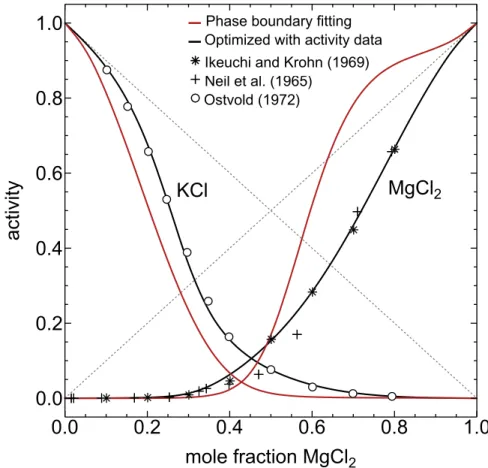
resulting activity vs. composition curves for KCl and MgCl₂ in molten KCl-MgCl₂ at 800 ∘C are shown in Fig 1-2 (in red). We may compare these activity curves with those calculated via fitting to both phase boundary points and emf measurements of the activities (in black) [70–72]; the emf data sets are denoted by their respective symbols. There is a clear discrepancy between the two calculations, with the results of the phase boundary optimization yielding poor agreement with the experimental activity data, particularly for MgCl₂.

KCl

MgCl

₂

Phase boundary fitting Optimized with activity data Ikeuchi and Krohn (1969) Neil et al. (1965) Ostvold (1972)

0.0

0.2

0.4

0.6

0.8

1.0 activity

0.0

0.2

0.4

0.6

0.8

1.0 mole fraction MgCl

₂

Figure 1-2: Activity vs. composition curves for KCl and MgCl₂ in molten KCl-MgCl₂ at 800 ∘C. The activity curves calculated via fitting of the phase boundary points in Fig. 1-1 are in red. In black are the activity curves calculated via fitting to both phase boundary points and emf measurements of the activities [70–72]; the emf data are denoted by their respective symbols.

It is not unreasonable to claim, therefore, that empirically-determined activity coefficients remain critical for thermodynamic modeling of ionic melts. The absence of these data is arguably the greatest bottleneck for the study of molten state materials, particularly for electrolysis reactions. As such, experimental methods for accessing

(34)

component activity coefficients are key for the rational design of molten electrolytes.

1.1.4 Experimental Methods for Measuring Solution

Ther-modynamics of Molten Electrolytes

Vapor Pressure and Cryoscopy

If the vapor pressure (assumed to be equal to the fugacity) at temperature 𝑇 of a component AX over pure (liquid) AX is known, then the activity coefficient 𝛾AX may

be calculated from the measured partial pressure of AX over the solution following:

𝑝AX/(𝑝0AX𝑥AX) = 𝛾AX. Various techniques have been employed to measure the vapor

pressure of molten salt species (see [43, 73, 74] for overview), and these are generally categorized as: direct pressure measurements via a gauge (and also of the boiling point) [20, 75–77]; transpiration measurements, in which a known amount of an inert carrier gas is passed over the liquid, and the mass of condensed vapor that was carried by the inert gas is related to its partial pressure [78, 79]; and effusion measurements, in which the rate of evaporation (via mass loss) of a vapor under ballistic transport conditions is related to its partial pressure [80, 81]. Measurement of thermodynamic activities is made difficult by the presence of associated species in the gas phase, such as dimers or trimers of salt compounds. For this method to be successful, the speci-ation in the vapor must be well known. For multicomponent systems, measurement accuracy suffers due the number of vapor species.

Cryoscopy refers to a type of measurement that relies on the equilibrium between a pure solid component AX and a molten salt solution [43, 73, 82]. It is termed “cryoscopic” by the fact that the addition of AX (insoluble in the solid state) to a solution at an invariant equilibrium for a given temperature will decrease the equi-librium temperature of that system, e.g., the addition of AX to a eutectic mixture at the eutectic temperature. However, this definition is somewhat relaxed when applied to the measurement of thermodynamic activities, as it does not strictly require the solution to be at an invariant point. By equating the chemical potentials of AX in the solid and liquid phases, one may show that 𝑑 ln 𝛾AX/𝑑(1/𝑇 ) = −Δℎfus,AX/𝑅, where

(35)

Δℎfus,AXis the enthalpy of fusion of pure AX. The cryoscopic determination of

activ-ity coefficients therefore requires calorimetric measurements of enthalpies of fusion. They also require that the composition of interest be saturated with respect to a component AX, limiting the concentration range over which 𝛾AX may be calculated.

Electrochemical Methods

Before discussing the electrochemical methods that have been employed to measure activity coefficients, it is important to define the relation between the relevant measur-able quantity, i.e., voltage, and the activities of the species in the electrolyte. Unlike vapor pressure and cryoscopic techniques, electrochemical methods directly probe the interaction of ions at the interface between a conductor and a dielectric. The equilib-ria (or non-equilibequilib-ria) at these interfaces are defined by these charged entities. This perspective must be reconciled with the understanding that chemical potentials can be measured only for electroneutral species2 and that it is the convention of thermo-chemical data to define the activity of solution components with respect to neutral compounds.

The point here may best be addressed through an example. One can consider a reaction of the type O + 𝑛e− → R, where O is a cation in solution and R is the reduced state of that cation, e.g.,

Pb2++ 2e− → Pb (1.4)

in a hypothetical system PbCl2-ACl, where ACl is a supporting electrolyte. However,

in defining values of the cell potential that invoke the activity of the electroneutral

2_{This is due to the constraint of electroneutrality. Cations and anions cannot be added}

indepen-dently of one another to a molten electrolyte, therefore the per atom Gibbs energy change of adding an ion cannot be determined. Though activity coefficients and chemical potentials of ionic entities may be defined mathematically, such quantities can only be measured for neutral components. It is a point of some subtlety which has led to confusion in the literature. A particularly revealing instance is a set of published exchanges in the 1970s between Elliott [83] and Grjotheim (and his supporters) [84, 85] regarding the solution thermodynamics of metallurgical slags. Grjotheim, in rigorously observing an electroneutral definition of the activity coefficient, came out ahead in this disagreement.

(36)

species PbCl2, one might turn instead to a different formulation of the reaction:

PbCl2+ 2𝑒− → Pb(𝑙)+ 2Cl−. (1.5)

This reaction does not follow the convention O + 𝑛e− → R, which has consequences, for example, in how one might mathematically describe the current-potential relation for that reaction. Furthermore, it seems to suggest that PbCl2 is an entity distinct

from Cl−, when in truth PbCl2 may be entirely dissociated. An equivalence must be

formally established between these two forms of the reaction, the former (Eq. 1.4) ex-pressing the electrode reaction as it exists in reality, and the latter (Eq. 1.5) exex-pressing the electrode reaction as we wish to model it with regards to solution thermodynam-ics.

Establishing this equivalence requires introducing a reference potential, such as that formed by the reaction

Ag++ e− → Ag. (1.6)

For simplicity, it is assumed that the reference electrolyte is AgCl-BCl, where BCl is a supporting salt. The net reaction is then

Pb2++ 2Ag → Pb + 2Ag+. (1.7)

At equilibrium, the cell voltage 𝐸cell is equal to the difference in the electrochemical

potential of the electrons in Pb and Ag [86]:

𝐸cell = 1 𝐹 (︁ 𝜇Ag_e− − 𝜇Pb_e− )︁ . (1.8)

The 𝜇e− are related to the electrochemical potential of the metal electrodes Pb and

Ag by: 𝜇Pb= 𝜇AClPb2++ 2𝜇Pb_e− 𝜇Ag= 𝜇BClAg+ + 𝜇 Ag e− (1.9)

(37)

where the superscripts ACl and BCl denote the “working” and “reference” elec-trolytes, respectively. The chemical potentials of the components PbCl2 and AgCl

may be written as [87]: 𝜇PbCl2 = 𝜇 0 PbCl2 + 𝑅𝑇 ln 𝑎PbCl2 = 𝜇 ACl Pb2++ 2𝜇 ACl Cl−

𝜇AgCl= 𝜇0AgCl+ 𝑅𝑇 ln 𝑎AgCl = 𝜇BCl_Ag+ + 𝜇BCl_Cl−.

(1.10)

Combining Eqs. 1.8, 1.9, and 1.10 yields:

𝐸cell = 1 𝐹 (︁ 𝜇Ag− 𝜇0AgCl )︁ − 1 2𝐹 (︁ 𝜇Pb− 𝜇0PbCl2 )︁ −𝑅𝑇 𝐹 ln 𝑎AgCl 𝑎1/2_PbCl₂ − 1 𝐹 (︁ 𝜇ACl_Cl−− 𝜇BCl_Cl− )︁ = 𝐸_cell0 −𝑅𝑇 2𝐹 ln 𝑎2 AgCl 𝑎PbCl2 − 1 𝐹 ∫︁ ACl BCl 𝑑𝜇_Cl− (1.11) where 𝐸0

cell is the standard state cell voltage for the reaction in Eq. 1.7. The integral

term is the junction potential, and it is the contribution to the cell voltage due to the variation in the chemical potential of the chloride ion between solutions PbCl2-ACl

and AgCl-BCl. If the cell is without transference of species between the working and reference electrolytes, then the junction potential is zero and 𝐸cell is directly a

function of the activities of the electroneutral compounds PbCl2 and AgCl. If the

junction potential is non-zero, it may be calculated for known concentration profiles of the electroneutral compounds [87]. The derivation leading to Eq. 1.11 provides a rigorous justification for how measured voltages are connected to the thermodynamic activities of electroneutral solution components in molten electrolytes.

Electrochemical methods are arguably the most direct means of studying the activity coefficients of ionic melts, as they may be done in situ and over a wide range of compositions and temperatures, provided suitable electrodes can be used. These methods may be classified into two groups: those which rely on a measurement of the electromotive force between two electrodes in a cell and are done under conditions of zero current, and those which are voltammetric, i.e., rely on the passage of current between two electrodes in the cell to generate current-potential curves. An overview

(38)

of each is provide below.

The electromotive force (emf) is the difference in the electric potential of two electrochemical interfaces, the electrons of which are in equilibrium with the charged species in their respective electrolytes. A number of electrochemical cell types suitable for emf measurements may be defined. These generally fall into two categories: cells with and without transference, defined as the “transfer” of electrolyte species between the two subsystems that comprise the cell [43, 87]. A typical cell without transference is a formation cell, in which the two electrodes are immersed in the same electrolyte and the formation potential 𝐸cell = Δ𝐺rxn/𝑛𝐹 of some component of the electrolyte

is measured. An example is Na|NaCl|Cl2. The majority of cells relevant for the study

of multicomponent molten electrolytes are those with transference. An example is an electrochemical cell of the type

A|AX𝑛, BX‖CX𝑚, BX|C. (1.12)

The emf is given by

𝐸cell = 𝐸cell0 − 𝑅𝑇 𝐹 ln 𝑎1/𝑚_CX 𝑚 𝑎1/𝑛_AX_𝑛 + Δ𝜑junction (1.13)

Calculation of the activity coefficient of CX𝑚 requires knowing 𝐸cell0 , Δ𝜑junction, and

𝑎AX𝑛. In general, the junction potential between two electrolyte solutions S

(1)

and S(2) containing 𝑛 ionic species is given by

Δ𝜑junction= 𝑅𝑇 𝐹 ∫︁ S(2) S(1) 𝑛 ∑︁ 𝑖=1 𝑡𝑖 𝑧𝑖 𝑑 ln 𝑎𝑖 (1.14)

where 𝑡𝑖 is the transference number3 of the 𝑖th ion and 𝑧𝑖 is the charge.

Numerous studies of emf measurements in molten electrolytes have been published

3_{The transference number 𝑡}

𝑖of an ion is the fraction of the current carried by that species between the working and reference electrolytes. It is a measure of the velocity of that ion relative to a reference velocity. In aqueous electrolytes, the solvent itself, water, is an obvious choice of a reference frame. However, for molten systems, in which the notion of a solvent is largely concentration-dependent or ill-defined, it is more appropriate to specify one of the ions as a reference, e.g., Cl− in a molten chloride [87].

(39)

(see [43], [87], [88], [89] and references therein). Emf investigations of thermodynamic activities are advantageous for the precision with which electrode potentials may be measured (on the order of microvolts). In addition, the magnitude of the emf increases with the ratio of the activities in Eq. 1.13, favoring the study of dilute solution com-ponents, where, for example, 𝑎CX𝑚 ≪ 𝑎AX𝑛. A limiting feature of emf measurements,

however, is the availability of stable reference potentials in high temperature molten electrolytes. Outside of select halide melts, comparatively few reference electrodes have been evaluated. In addition, the use of ion selective membranes may also be problematic, particularly in molten oxides and sulfides, due to the reactivity of the electrolyte.

Voltammetric methods of measuring thermodynamic activities rely on the gen-eration and interpretation of characteristic current-potential (𝑖-𝐸) curves. These measurements are inherently non-equilibrium in nature due to the generation of net current in the cell. In order to establish a quantitative connection to the activity coefficient of a solution component, the non-equilibrium contributions to the mea-sured voltage must be known or made negligible. Under conditions of net current, the measured cell voltage 𝑈 is given by:

𝑈 = 𝐸cell+ 𝑖𝑅u+ 𝜂mt+ 𝜂act (1.15)

where 𝐸cell is the equilibrium cell voltage (e.g., Eq. 1.11) under zero-current

condi-tions, 𝑖 is the current, 𝑅u is the uncompensated resistance of the cell, 𝜂mt is the mass

transport overpotential, and 𝜂act is the activation overpotential of the cell. For a

two-electrode configuration (anode and cathode), the overpotential terms in Eq. 1.15 rep-resent non-equilibrium processes at both the anode and cathode. If a three-electrode cell is employed, consisting of a working electrode (WE), a reference electrode (RE), and a counter electrode (CE), and the potential of the WE is measured against that of the RE, the overpotential contributions in Eq. 1.15 are due to the WE reaction alone. Both 𝜂mtand 𝜂actare functions of 𝑖. Eq. 1.15 is therefore a generalized representation

(40)

how-ever, to define 𝑖 with respect to 𝐸. A number of formulations of 𝑖 ≡ 𝑓 (𝐸) have been derived, depending on the mass transfer conditions and the electron transfer kinetics at the WE electrode surface. The expressions implicitly account for the overpotential contributions in Eq. 1.15. General commonalities about 𝑖-𝐸 relations in voltammetry include the following. Transport of electroactive species to the WE surface is pro-portional to the current, and it is often assumed to be diffusion-controlled, whereby Fick’s 2nd law may be used to model the concentration as a function of time and position. The boundary conditions are geometry-dependent, with planar, cylindrical, and spherical diffusion profiles being common. Where appropriate, electron transfer kinetics are typically described by elementary rate theory (e.g., the Butler-Volmer equation). Mathematical models of the 𝑖-𝐸 relation are compared with measured data to calculate reaction parameters such as active surface area, diffusivity, and con-centration, as well as characteristic electrode potentials (e.g., the half-wave potential

𝐸1/2) from which activity coefficient data may be determined. The comparison

re-lies on correlating specific features of the 𝑖-𝐸 curve, or waveform, such as extrema points, inflection points, and asymptotic regions, to the corresponding mathematical expression of that waveform feature.

The functional form of the 𝑖-𝐸 relation is specific to the potential or current program applied to the working electrode. These may be categorized as being either steady-state or transient.

Steady-state techniques include polarography (at a dropping liquid metal elec-trode, e.g., Hg) [90] and sampled-current voltammetry [91]. For an electrochemically-reversible reaction O + 𝑛e−↔ R (O and R soluble) under conditions of semi-infinite linear diffusion, the 𝑖-𝐸 relation is given by the Heyrovsky-Ilkovic equation [92]:

𝐸 = 𝐸1/2− 𝑅𝑇 𝑛𝐹 ln 𝑖 − 𝑖d,ox 𝑖d,red− 𝑖 (1.16)

where 𝐸_1/2 is the half-wave potential and 𝑖d,ox, 𝑖d,red are the diffusion-limited currents

(Cottrell currents) for the oxidation and reduction reactions, respectively. When

(41)

coefficients of O and R by: 𝐸1/2 = 𝐸0′− 𝑅𝑇 𝑛𝐹 ln 𝐷_O1/2 𝐷_R1/2 = 𝐸 0₋ 𝑅𝑇 𝑛𝐹 ln 𝛾R𝐷O1/2 𝛾O𝐷 1/2 R (1.17)

where 𝐸0′_{is the formal potential of the reaction and 𝐸}0 _{is the standard state reaction}

potential. Though Eq. 1.16 is applicable to steady-state voltammetry in certain elec-trolysis reactions, it is more common to encounter molten systems where the reduced species R is insoluble in the electrolyte. In such cases, the 𝑖-𝐸 relation is described by the Kolthoff-Lingane equation [93]:

𝐸 = 𝐸1/2− 𝑅𝑇 𝑛𝐹 ln 1 𝑖 − 𝑖d,red . (1.18)

Eqs. 1.16 and 1.18 have been applied to calculate half-wave potentials and standard state potentials of reduction reactions in a variety of molten electrolytes [88, 89, 94– 97].

For the reaction O + 𝑛e− ↔ R, if the concentration of electroactive species is high or there is convection at the electrode surface minimizing mass transfer overpotential (concentration polarization), the 𝑖-𝐸 relation at potentials far from the half-wave po-tential tends to be linear with a slope of 𝑅−1_u . The reduction or oxidation potential is then estimated by extrapolation of the linear portion of the 𝑖-𝐸 curve to the potential at zero current [88, 98, 99].

Chronopotentiometry [100] is a transient electroanalytical technique that has been used to measure the reaction potentials of decomposition reactions in molten elec-trolytes [95, 97, 101, 102]. In this method, constant current (galvanostatic) electroly-sis is applied at 𝑡 = 0 in the absence of convection, and the time 𝜏 required to reach complete concentration polarization (𝜂mt → ∞) is recorded. For an

electrochemically-reversible reaction, one may show that the measured potential is related to 𝜏 by the following: 𝐸 = 𝐸𝜏 /4− 𝑅𝑇 𝑛𝐹 ln 𝑡1/2 𝜏1/2_{− 𝑡}1/2 (1.19)

(42)

where 𝐸𝜏 /4 = 𝐸0− 𝑅𝑇 𝑛𝐹 ln 𝛾R𝐷 1/2 O 𝛾O𝐷 1/2 R . (1.20)

The quarter-wave potential 𝐸𝜏 /4 is analogous to the half-wave potential of

steady-state voltammograms (Eq. 1.17). For reactions where the product R is insoluble, the

𝑖-𝐸 relation is instead given by [103]: 𝐸 = 𝐸0′+ 𝑅𝑇 𝑛𝐹 ln (︁ 𝜏1/2− 𝑡1/2)︁ +𝑅𝑇 𝑛𝐹 ln (︃ 2𝑖0 𝑛𝐹 𝐴(𝜋𝐷O)1/2 )︃ . (1.21)

where 𝑖0is the applied current and 𝐴 is the active surface area of the WE. As a means

of measuring reaction parameters, chronopotentiometry is more accurate than steady-state voltammetry. However, for the purpose of identifying thermodynamic activities from reaction potentials, it has not found much favor in the literature. This is a result of the fact that measurements of 𝜏 require a relatively large potential window in order to avoid activating additional redox reactions, and this is often unavoidable in multicomponent electrolytes.

Transient voltammetry techniques include linear sweep voltammetry (LSV), cyclic voltammetry (CV), square-wave voltammetry (SWV), and alternating current voltam-metry (ACV). Correlations between waveform peaks and the reaction potential have been used to calculate standard state Gibbs energies and component activities for a number of electrolyte systems [104–113]. Details on the 𝑖-𝐸 relations for each tech-nique may be found in the relevant references [24, 91, 114]. It is outside the scope of this writing to provide a detailed description of these methods. However, it is valuable here to bring attention to those studies that have specifically considered re-actions involving insoluble reaction products, this being the class of rere-actions that best describes electrolytic decomposition in molten systems. Berzins and Delahay [115] first derived the 𝑖-𝐸 relation for reversible metal deposition under the condi-tions of a linear DC potential sweep starting at the open circuit potential. It may be shown the potential of the reduction peak current is expressed as

𝐸peak= 𝐸0− 𝑅𝑇 𝑛𝐹 ln (︃ 1 𝛾O𝐶O* )︃ − 0.834𝑅𝑇 𝑛𝐹 (1.22)

(43)

thereby providing a connection between the peak potential and the activity coefficient of the solution component O. The extension of the theory of Berzins and Delahay to arbitrary switching potentials, i.e., for the full cyclic voltammogram, was later made by Lantelme and Cherrat [116]. Berghoute et al. [105] applied this theory to measure the standard reduction potentials of Cl2/Cl−, Pt2+/Pt0, and Ni2+/Ni0 in equimolar

NaCl-KCl, under the assumption that the salt component being reduced behaves ideally (𝛾O = 1). Nakanishi and Allanore were the first to show that ACV can be

used calculate decomposition potentials in molten electrolytes. Empirical correlations were made between the peak potentials of the ACV harmonic waveforms and the cell voltage to estimate the partial Gibbs energies of molten alumina [117] and of La2O3

-Y2O3 [118].

1.2 The Argument for a Voltammetric Approach

to Measuring Thermodynamic Activity

Coef-ficients

The rational design of molten electrolytes for electrolytic processes requires knowl-edge of the mixing thermodynamics, as captured by the activity coefficients of the solution components, in order to predict decomposition potentials, liquidus temper-atures, phase stability, etc. The thermodynamic models (Section 1.1.2) that afford predictive capability for designing such electrolytes remain reliant upon empirically-determined activity measurements. The activities of solution components in ionic melts have been studied by several methods (Section 1.1.4). The most widespread of these are electrochemical in nature. An electrochemical approach to measuring thermodynamic activities has the advantage of requiring fidelity to the actual ionic speciation present in the electrolyte, of being executable in situ, of being relatively simple to perform, and of being generally applicable over a wide range of compositions and temperatures.

(44)

most prevalent method of measuring activity coefficients in electrochemical systems. However, in high temperature ionic melts, emf measurements become less attractive due to the limited availability of known reference electrodes and the reactivity of the electrolyte, which may preclude the use of ion-selective membranes or porous separa-tors. In addition, emf measurements commonly require that the equilibrium reactions defining the cell voltage be present for the duration of the experiment. Though elec-trolytic generation of the required products may be done in situ, immediately prior to the emf measurement, to establish the appropriate electrode potentials, this puts additional constraints on the design of the cell (see the “commutator” method in [88]). A voltammetric approach to the measurement of thermodynamic activities has its own challenges. Foremost among them is the fact that it is a non-equilibrium technique, requiring an accounting of the overpotential contributions to the 𝑖-𝐸 re-lation (see Eq. 1.15). The data analysis is inherently more complicated than for an emf measurement and introduces the possibility of greater uncertainty. However, voltammetry is advantageous in that it may be done in the absence of junction po-tentials arising from the use of membranes, separators, etc., if a “dynamic” reference electrode is employed in the same electrolyte making use of a gas-evolving anodic reaction [117, 119]. An example is O2/O2− in a molten oxide. The generation of

the electroactive species that establish the WE potential may also be done during the measurement itself, simplifying its execution. In addition, it is well established that voltammetry, particularly transient techniques such as CV and ACV, excels at providing diagnostic insight into the electrode reactions. Though not the primary focus of this work, reaction mechanisms and transport properties are accessible with such measurements, and lends them a degree of analytical utility not shared by emf measurements. The above capabilities make voltammetry, as a method for quanti-tative determination of activity coefficients in molten electrolytes, worth pursuing as an alternative approach to emf measurements.

Of the various voltammetry methods (see Section 1.1.4), only DC cyclic voltamme-try has been applied to modeling electrolysis reactions in molten systems, specifically via the theoretical work of Berzins and Delahay [115], and Lantelme and Cherrat

(45)

[116]. It is known, however, that reproducible DC cyclic voltammograms that may be readily interpreted by analytic solutions to the current-potential relation are diffi-cult to capture in high temperature molten systems [5, 117, 120]. This may be due to convection or the absence of significant mass transport overpotential, giving rise to anodic and cathodic currents that lack well-defined 𝑖-𝐸 extrema. Determination of reaction potentials from these waveforms relies on a questionable extrapolation to the potential at null-current. In comparison, AC voltammetry of electrolysis reactions has been shown to yield well-defined 𝑖-𝐸 extrema that may be correlated with electrode reaction potentials [117]. The development of an ACV theory of electrolysis reactions that maintains the same analytical capability demonstrated for soluble reduction-oxidation couples in aqueous systems would provide the electrochemist with a novel approach to measuring the thermodynamic properties of molten electrolytes.

It is the focus of the present work to motivate a voltammetric approach to investi-gating the solution thermodynamics of molten electrolytes. Specifically, the qualities of ACV that afford it such utility as an electroanalytical technique (superior dis-crimination against double layer charging current, increased sensitivity to reaction kinetics, Fourier analysis, etc.) warrant its extension to the study of high temper-ature molten systems. As such, this work explores the use of ACV for measuring activity coefficients in high temperature ionic melts.

1.3 Background on Alternating Current

Voltam-metry

1.3.1 Prior Art

Alternating current voltammetry became an active area of research in the 1940s through the efforts of Breyer and Gutmann [121–123], Grahame [124], Ershler [125], and Randles [126] to provide theoretical treatments of the response of an electrochem-ical reaction to an alternating potential perturbation. There emerged two approaches to measuring and describing the response of an electrochemical cell to an alternating

Alternating current voltammetry of high temperature electrolysis reactions

Alternating Current Voltammetry of High

Temperature Electrolysis Reactions

by

Andrew Harvey Caldwell

Submitted to the Department of Materials Science and Engineering

in partial fulfillment of the requirements for the degree of

Doctor of Philosophy

at the

MASSACHUSETTS INSTITUTE OF TECHNOLOGY

February 2020

c

○ Massachusetts Institute of Technology 2020. All rights reserved.

Author . . . .

Department of Materials Science and Engineering

January 6, 2020

Certified by . . . .

Antoine Allanore

Associate Professor of Metallurgy

Thesis Supervisor

Accepted by . . . .

Donald R. Sadoway

John F. Elliott Professor of Materials Chemistry

Chairman, Departmental Committee for Graduate Studies

Alternating Current Voltammetry of High Temperature

Electrolysis Reactions

by

Andrew Harvey Caldwell

Abstract

Acknowledgments

Contents

List of Figures

List of Tables

List of Symbols

Chapter 1

Introduction

1.1

Background on Molten Electrolytes

1.1.1

Structure of Molten Electrolytes

1.1.2

Solution Models of Molten Electrolytes

1.1.3

Limitations of Phase Boundary Fitting for Activity

Cal-culations in Molten Electrolytes

KCl

MgCl

0.0

0.2

0.4

0.6

0.8

1.0

activity

0.0

0.2

0.4

0.6

0.8

1.0

mole fraction MgCl

1.1.4

Experimental Methods for Measuring Solution

Ther-modynamics of Molten Electrolytes

1.2

The Argument for a Voltammetric Approach

to Measuring Thermodynamic Activity

Coef-ficients

1.3

Background on Alternating Current

Voltam-metry

1.3.1

Prior Art