Analysis of electron beam-plasma systems.

1,14

ANALYSIS OF ELECTRON BEAM-PLASMA SYSTEMS

TECHNICAL REPORT 423

JULY 31, 1964

MASSACHUSETTS INSTITUTE OF TECHNOLOGY

CAMBRIDGE, MASSACHUSETTS DOCUIi * W V)FiCE 2 3 27

E, S - G -, : .E. - . ' V ,;:,', Oi F ELECTRON!CS

CM' SS"i"' E i-it 02139, U.SNOLOGYA.

*et_

The Research Laboratory of Electronics is an interdepartmental laboratory in which faculty members and graduate students from numerous academic departments conduct research.

The research reported in this document was made possible in part by support extended the Massachusetts Institute of Technology, Research Laboratory of Electronics, jointly by the U.S. Army (Electronics Materiel Agency), the U.S. Navy (Office of Naval Research), and the U.S. Air Force (Office of Scientific Research) under Contract DA36-039-AMC-03200 (E); and in part by Grant DA-SIG-36-039-61-G14; additional support was received from the National Science Foundation (Grant G-24073).

Reproduction in whole or in part is permitted for any purpose of the United States Government.

MASSACHUSETTS INSTITUTE OF TECHNOLOGY

RESEARCH LABORATORY OF ELECTRONICS

Technical Report 423 July 31, 1964

ANALYSIS OF ELECTRON BEAM-PLASMA SYSTEMS

Philip E. Serafim

This report is based on a thesis submitted to the Department of Electrical Engineering, M. I. T., October 14, 1963, in partial ful-fillment of the requirements for the degree of Doctor of Science.

(Manuscript received February 3, 1964)

Abstract

The interaction between an electron beam and a plasma in metallic waveguides and in the presence of an external longitudinal magnetostatic field is analyzed. Plasma ions and electrons are considered. The treatment refers to a temperate plasma. By use of a multispecies theory, the treatment may be extended to warm plasmas. The electron beam is rectilinear and has a well-defined unperturbed velocity. This velocity is assumed to be uniform over the waveguide cross section. Modifications for nonuniform velocity are also presented. The treatment is valid for slow and fast waves and for rel-ativistic beam velocities.

In the first part an exact analysis is made of the beam-plasma waveguide based on the linearized Maxwell equations and the Lorentz force equation. The "operator" die-lectric tensor description of the beam-plasma medium is introduced. The properties of this tensor are examined and the boundary conditions are formulated in terms of the ele-ments of this tensor. The field analysis for the beam-plasma system is made, and the dispersion equation and the determinantal equations are derived from the satisfaction of the boundary conditions. Cutoffs, resonances, slow waves, and the quasi-static approx-imation are studied. Conservation principles for our specific beam-plasma system are formulated, and Chorney's bidirectional theorem is extended to our medium. Some var-iational theorems for this system are also studied.

In the second part a solution of the plasma waveguide problem by a coupling-of-modes theory is given. The theory of coupling of empty-waveguide coupling-of-modes and quasi-static modes for the approximate description of a general gyrotropic medium is formulated. The results are specialized for plasma waveguides, and the case of a completely filled circular plasma waveguide is examined in detail.

TABLE OF CONTENTS

I. INTRODUCTION 1

1. 1 History of the Problem 1

1.2 Analysis of the Beam-Plasma System 3

1.3 Outline of the Analysis 5

II. DIELECTRIC TENSOR 7

2. 1 Introduction ₇

2.2 Operator Mobility Tensor ₇

2.3 Operator Dielectric Tensor 10

2. 4 Transverse Variation of DC Velocity and Charge Density 14

2. 5 Properties of the Dielectric Tensor 16

2. 6 Boundary Conditions 17

2. 7 Warm Plasmas ₂₀

2. 8 Special Cases ₂₂

III. FIELD ANALYSIS AND CONSERVATION PRINCIPLES 26

3. 1 Introduction 26

3. 2 Relation between the Longitudinal Fields 28

3.3 Transverse Fields 30

3.4 Field Solution and Dispersion Relation 32

3. 5 Critical Frequencies and Slow Waves 34

3. 6 Quasi-static Approximation 37

3. 7 Conservation Principles for the Operator Tensor Medium

Description of the System 41

3.8 Variational Theorems ₄₆

IV. COUPLING OF EMPTY-WAVEGUIDE MODES AND QUASI-STATIC

MODES IN WAVEGUIDES LOADED WITH GYROTROPIC MEDIA 50

4. 1 Introduction 50

4. 2 Coupled-Mode Theory ₅₁

4. 3 Uncoupled Modes ₅₃

4. 4 Coupling Coefficients 56

4. 5 Dependent Coupling Equations 59

4.6 Dispersion Relation 61

4. 7 Plasma Waveguides 63

4. 8 Circular Cylindrical Geometry 64

4. 9 Example 70

V. CONCLUSIONS 78

CONTENTS

Appendix A Single Electron Beam 80

Appendix B Special Geometries 83

Appendix C Properties of Empty-Waveguide Modes 87

Appendix D Modified Bessel Functions 89

Appendix E Completely Filled Plasma Waveguide 92

Acknowledgment 93

References 94

I. INTRODUCTION

1. 1 HISTORY OF THE PROBLEM

The theory of beam-type microwave tubes is concerned with the interaction of a beam of drifting electrons either with stationary electric fields (gap systems) or traveling electromagnetic waves (traveling-wave tubes, and so forth). In the latter case the waves are supported by metallic circuits. Such traveling waves could just as well be supported by a system consisting of a plasma and a metallic waveguide. In such devices we are then confronted with the problem of beam-plasma interaction. Recently there has been extensive research, both theoretical and experimental, on the interaction of a beam-plasma system, for the purpose of amplifying microwave power and of heating the plasma at the expense of the DC energy of the electron beam. The heating of plasma ions is of great importance for the achievement of controlled thermonuclear reaction.1 Although the interest in the beam-plasma interaction is rather recent, the problem itself is old. A beam-plasma interaction was originally suggested by Langmuir, in 1925. Very few papers on this subject were published between 1925 and 1948, after which a series of papers appeared that excited the interest of engineers and physicists.

The most important prediction resulting from this work was that in an infinite beam-plasma system a growing wave may arise which propagates for frequencies below the plasma resonance frequency, and it has maximum amplification near the plasma resonance.

The contributions to this research by Pierce and Bailey were very important. They predicted traveling-wave amplification for a system consisting of an electron beam drifting through an ion cloud.3 The research on the double-stream amplifier was also significant in this regard because the double-stream amplifier mechanism occurs quite frequently in beam-plasma interaction.4

About the same time, Bohm and Gross in a series of papers gave the most suc-cessful treatment of plasma oscillations. They considered electrons with thermal velocities in the plasma interacting with the electrons of a beam of well-defined velocity. They worked out this problem by using Maxwell's equations and the Lorentz force equation. They clarified the physical processes of the interaction and predicted that plasma oscillations must be excited by an electron beam sent through a homogeneous plasma. Several unsuccessful attempts were made to excite the growing wave by beam-plasma interaction.8 It has been suggested that the failure of these experiments was due to the amplification, which was too small for amplification of noise oscillations to an observable level.9 Finally, Boyd, Field, and Gould1 0 and Kharchenko and his co-workers 1 succeeded in exciting oscillations at the plasma resonance frequency.

The effects of boundaries had already been studied by Bohm and Gross. The effects of nonzero plasma electron temperature were first studied by Vlasov, 12 Landau,1 3 B;ohm and Gross,6 and Allis.1 4

1

The most detailed analysis of beam-plasma interaction was published by Allen and Kino 5 for a cylindrical system in a finite, axial magnetostatic field. A detailed

anal-ysis has also been made by Fainberg,1 6 who again made use of linearized equations. It has been suggested recently that we cannot always linearize the equations that describe

the system. Klimontovich and Silin1 7 in a recent chapter point out that the known

treatments of this problem are based, in essence, on the assumption that the particles entering the plasma do not change the properties of the plasma. The presence of the

Langmuir effect17 indicates that such an approach is not always sufficient. In such

cases a system of nonlinear equations for the electrons of the beam and of the plasma

must be solved simultaneously. Since the energy transfer from the beam to the wave

takes place in the region where the wave grows, the process of establishment of a wave must be examined.

Even when the linearized equations are used, the whole analysis becomes cumber-some, because of the complicated equations involved in the solution of the problem, and

the answers, once obtained, are numerical and cannot be generalized. Therefore we

need approximate approaches that would be simpler mathematically. A very powerful

approach is coupling-of-modes, which was introduced by Pierce.l8 This approach not only made general results available but also, when properly used, provided physical

insight to the problem. Its main drawback was that the approximation involved was

satisfactory only for weak coupling at various systems. This drawback was removed

by Haus. 19 By variational methods, he obtained a valid formalism for tightly coupled systems which reduces to Pierce's formalism for weakly coupled systems.

Another approximation technique was the quasi-static approach introduced by Smullin

and Chorney,2 0 and by Gould and Trivelpiece.2 1 Under the approximation V X E 0

an electric potential may be used. The solution of the problem and the results become

significantly simpler. A very important prediction in Smullin and Chorney's analysis

was the interaction between a backward wave above the plasma frequency in the finite plasma column and the electron beam by use of quasi statics and coupling of modes. They also point out that interactions predicted by the beam-plasma theory are analogous

to interactions that occur in various microwave tubes. The usefulness of the

quasi-static approximation is limited, because of the question about the region of its validity. Initially, it was thought to be valid for slow waves in general. Bers has proved2 2 that a rigorous analysis establishes additional restrictions.

We conclude this historical sketch by mentioning some of the experiments related to our problem. Boyd, Field, and Gould1 0 revealed a strong interaction of a modulated

beam with the plasma of a mercury arc discharge. Their results agreed with their

analysis based on the method of Bohm and Gross. Other successful experiments have

been performed by Tchernov, 3 and by Allen and Kino. 5 Experiments have been

24

reported in which an urimodulated electron beam stimulates ion oscillations, both ion

and electron oscillations,2 5 and electron oscillations in a system normally used for ion oscillations.26 Experiments by Smullin and Getty with a low-pressure gas-arc device

in the Research Laboratory of Electronics, M.I.T., have indicated interaction of an electron beam with plasma produced by the beam.27 This interaction produces large-signal oscillations. These experiments are being continued by Smullin, Getty, Hartenbaum, and Hsieh, with higher power input to the beam.

1.2 ANALYSIS OF THE BEAM-PLASMA SYSTEM

We now turn to a few of the problems in the broad field of beam-plasma systems to which we shall devote attention.

There are many approaches to the field analysis in an anisotropic medium. One of them is similar to the normal-mode expansion in isotropic waveguides. Very important

contributions to the development of this method have been made by Suhl and Walker,2 8 Kales,2 9 Gamo,30 and Van Trier31 who worked with gyromagnetic media. The first complete analysis for guided waves in anisotropic media was given by Van Trier.32 A thorough analysis for guided waves in gyroelectric media has been given by Bers.3 3

The most general approach to the problem of field analysis in anisotropic and inhomo-geneous media was given by Schelkunoff,3 4 by use of an approach quite different from that introduced by Kales.

For a linearized description of a system, which we shall examine, a powerful technique for the study of the exchange of energy between beam and plasma is the small-signal conservation principle introduced by L. J. Chu for an electron beam under the assumption of infinite magnetostatic field.35 This principle has been extended to a filamentary beam in finite magnetostatic fields by Bobroff and Haus.36 A power theorem for an electron beam and plasma by use of electromagnetic potentials was given

by Sturrock.37 Bers and Penfield formulated the conservation principle for a finite irrotational relativistic beam.38 Recently, Bobroff, Haus, and Kliiver generalized their principle for finite nonrelativistic beams in terms of polarization variables.3 9 Kliiver has also given the conservation theorem in terms of electromagnetic potentials.4 0

a. Theory and Models

We use a macroscopic treatment in which the basic equations describing the beam-plasma system are Maxwell's equations, the Lorentz force equation, and the conser-vation of charges. Because of their nonlinear character, we linearize them by using the small-signal theory. In this theory we assume that the total fields and mechanical variables are expressible as a superposition of a large unperturbed quantity (denoted by subscript o) and a very small perturbation (without subscript). Under this assump-tion, we may neglect quantities of second order in perturbed variables.

In general we shall not make the quasi-static assumption. That is, we consider the effect of the AC magnetic flux density on the curl of the AC electric field. Therefore our treatment is valid for slow as well as for fast waves. Since the quasi-static approach provides a useful tool in the region of its validity, we formulate the

quasi-static approximation to our problem and investigate this region.

In Section II and part of Section III the beam velocity is assumed to be relativistic for generality, although for most cases it is safe to assume that the beam velocity is much smaller than the velocity of light. That is the reason for giving the resulting simplifications (section 2. 8). The conservation principles in Section III are formulated for nonrelativistic beam velocities.

There is a uniform, finite, axial, magnetostatic field along the axis of uniformity of the waveguide. It is assumed to be much larger than the DC magnetic flux density resulting from the DC current of the beam.

The model that has been chosen for the plasma contains electrons neutralized in the unperturbed state by ions of finite mass. In some cases the effect of the ions may be neglected (section 2. 8). In general we assume uniform DC charge density for the plasma ions and electrons. Only in sections 2. 4-2. 6 do we examine cases with transverse variation of the DC charge density. In order to take into consideration the temperature of plasma electrons and ions we use a multispecies theory. In section 2. 7 we show how this multispecies theory may be used in the examination of initial temperature.

For the beam we assume electrons drifting along the axis of uniformity of the waveguide. The DC beam velocity is assumed in general to be uniform (except in sections 2. 4-2. 6 where transverse variation of the DC velocity is allowed). The beam electrons are neutralized by nondrifting ions of finite mass. The simplification for infinite ionic mass is given in section 2. 8. The DC charge density of the beam electrons is assumed in general to be uniform (except in sections 2.4-2. 6).

We neglect collisions of any kind throughout the whole treatment; we assume a loss-less beam-plasma system. The consideration of collisions would modify the elements of the dielectric tensor. The modified dielectric tensor may be used in Section III for the field analysis in the case of collisions.

The waveguide is assumed to be metallic, lossless, uniform with the z-axis taken along the axis of the waveguide. In general, the cross section of the wave-guide is arbitrary; thus we use a generalized system of transverse orthogonal coordinates. The waveguide is not necessarily filled by the plasma or the beam, nor does the plasma need to have the same cross section as the beam. For the extension of our theory in such cases we consider an abrupt change of the corresponding charge densities at such boundaries and the introduction of surface charges and currents (section 2. 6). In the actual system there is not, of course, such an abrupt change in charge densities; instead unneutralized sheaths are formed. The problem of guided-wave propagation in the presence of sheaths has not yet been solved.

Finally, we assume the various small signal quantities to be Fourier-analyzed in space and time. The z-dependence is taken as exp(-yz), where y = a + jp, and the time-dependence exp(jct), where w is always taken real. Hence our entire analysis

will be restricted to beam-plasma systems that are free of nonconvective (absolute) instabilities.

1.3 OUTLINE OF THE ANALYSIS

There are two basic ways of analyzing beam-plasma systems. One method is to follow a direct approach to the solution of the beam-plasma system considered as an entity; this is followed in Sections II and III. The second approach is the use of the coupled-mode theory. We consider the plasma as one entity and the beam as another and study their weak coupling. This has already been done by use of a quasi-static model for the plasma. The non quasi-static treatment of the plasma is known but mathematically complicated; therefore, in Section IV we give an approximate approach to the non quasi-static solution of the plasma alone by coupling of empty-waveguide and quasi-static modes.

In Section II we derive the tensor-medium description of the system that is used for the field analysis and the formulation of the characteristic equations of the system.

First, we derive the operator tensor relation between the velocities and the electric field. By use of this relation we derive the dielectric tensor, which contains operator elements. Thus we call it "operator" dielectric tensor. This tensor is slightly mod-ified when we allow transverse variation of charge densities and of the velocity of the beam. The newly formulated operator dielectric tensor is shown to be Hermitian for a lossless passive medium surrounded by lossless walls. Next, we deal with the proper boundary conditions derived from the tensor description of the medium, which must be used for the field analysis.

We demonstrate how the multispecies theory, which is used throughout this report, may be used for the adoption of our theory for the study of cases with finite electron and ion temperatures (some special cases are examined).

In Section III we give the field analysis, the characteristic equations of the beam-plasma system, and we deal with conservation principles for the beam-beam-plasma system.

We derive a set of second-order partial differential coupled equations for the lon-gitudinal fields, which may be transformed to a set of uncoupled fourth-order equations. Then the transverse fields can be found by use of their relations with the longitudinal fields. Because of the similarity (although the coefficients are modified) between the field analyses for a beam-plasma system and for plasma alone, we extend the tech-niques for the field solution and the derivation of the dispersion and determinantal equations from the latter system to the former system. (For a better physical under-standing of the resulting equations (field solution and dispersion equation in section 3.4; determinantal equation in Appendix B) we examine the simple case of a single electron beam (Appendix A).)

We give the simplifications that may be made for the critical frequencies of the system and for the important region of slow waves. We also give the simplifications that result under the quasi-static approximation and we examine the region of its validity.

5

-Then we give the logical extension to our system of Chorney's theorem for bidirec-tional waveguides in terms of the dielectric tensor and the electrical variables only. Finally, we give variational theorems for the beam-plasma system. We treat also a few examples.

It has been observed that the non quasi-static plasma modes behave as quasi-static modes near resonances and as empty-waveguide modes near cutoffs. This suggests an approximate approach to the non quasi-static solution of the plasma based upon the coupling of empty-waveguide modes and quasi-static modes. This is accomplished in Section IV.

For generality we deal with a gyrotropic medium and examine the coupling of empty-waveguide modes to quasi-static modes. In section 4.3 and Appendix C we review the

properties of the empty-waveguide modes and derive the orthogonality conditions and the normalization for the quasi-static modes. Then we derive the coupling coefficients for a gyrotropic medium, whose dielectric tensor and magnetic permeability are functions of space. Next, we discuss the dispersion relation.

After the formulation of the general theory we specialize the results of sections 4.4 and 4. 5 for a plasma that may not fill the waveguide completely. We apply our suggested procedure for a circular cylindrical geometry (section 4. 8, Appendix D). Then we pre-sent an example of a completely filled waveguide, and compare the results obtained by use of the coupled-mode theory with the results found by direct solution of the problem of a plasma waveguide (Appendix E).

II. DIELECTRIC TENSOR

2. 1 INTRODUCTION

Our purpose here is to show how the whole system (electron beam and plasma) can be described as an anisotropic dielectric medium. First, we examine the general non quasi-static and relativistic case, and then we give the simpler forms reduced under certain assumptions.

In section 2. 2 we derive the mobility tensor for each species according to our multi-species theory. The mobility tensor for the mth multi-species relates the AC velocityVm to

the AC effective electric field E + v X B. We wish to find the mobility tensor relating om

Vm and E only. We must eliminate B; since B is related to E through differential operators, the final mobility tensor will contain differential operators.

In section 2. 3 we derive the dielectric tensor under the assumption of homogeneous DC charge density and velocity. The case of transverse variation of the DC charge density and velocity is examined in section 2. 4. The time derivative of the dielectric displacement vector is equal to the time derivative of EoE plus the convection current of each species (which is a function of the AC charge density and velocity). Both of these quantities are related to E through differential operators. Therefore the dielectric displacement vector is related to E through differential relations. Since the dielectric displacement vector is equal to E premultiplied by the dielectric tensor, this tensor must contain differential operators. In section 2. 5 we examine the properties of the dielectric tensor.

In section 2. 6 we study the boundary conditions necessary for the solution of the problem of wave propagation in the system. We show how the boundary conditions are satisfied because of the operational character of the dielectric tensor. For a waveguide partially filled by plasma and/or beam, the sheath around the column of plasma and/or beam must be taken into consideration in a rigorous solution. In this treatment we neglect the effect of sheaths.

Throughout we make use of the multispecies theory because our theory may be adopted for the study of cases with nonzero electron and ion temperatures. Without elaborating on this subject we show how it may be accomplished in section 2.7.

In section 2. 8 we examine some special cases: the cases of plane waves, infinite ion mass, infinite magnetostatic field, temperate plasma and beam, and nonrelativistic beam velocity. (The term "temperate" was introduced by Allis.4 1 )

The model which will be used in the analysis has already been described in section 1.2.

2.2 OPERATOR MOBILITY TENSOR

The Lorentz force equation for the mth species is written

7

-d

dt (mV)m = e(E+ VX B) . (1)

We have assumed that there is a DC magnetic field Bo along the z-axis. The DC

velocity VoM of each species is also z-directed. By use of the small-signal theory under

the above-mentioned assumptions we find3 8 that

(m)m = mTmVTm + mzmvzm. (2)

Here, mTm and mzm denote the unperturbed "transverse" and "longitudinal" masses.42

mTm _mTm mm Rm _momRom (3) m _Zm = m _{om om'}Rm3 (4) where 1 2 -1/2 Rom = We find also (E+ vX B)m = E + Vom X BT + VTm X B (5) Let us define e o m B (6) cm m o0

We assume that all AC quantities vary as f(ul,u 2) exp(jwt-yz), where f(u1,u2) is a function of the transverse coordinates. We also assume that the DC velocity of each species has no transverse variation.

We introduce Eqs. 2, 5, and 6 into Eq. 1 and separate (1) into transverse and lon-gitudinal components. Finally, we get

mTm(jw-yvom+ocmizX) VTm = em(ET+Vom X BT ) (7)

m _{mzm(j-Om) zm} (j~- =e E. _emEZ (8)₍₈₎

The solution of Eqs. 7 and 8 is

V = jm (E+VomX BT), (9)

where M -jM 0 M1 m Jxm m M xm m ° . (10) 0 0 MII m Let us define X _rm =( + jyv _om (11) e m 'm=m (12) om

The elements of the mobility tensor4 3 Mm are given by

MIm rTm R (13)

m2 ) Om (2c -)m

cm rmcm rm

cm tm cm

xm _{nxm (co2}

TOm

-Cm rm cm -orm

1 m 1 (15)

= - (15).

im -zm rm R3 rm

om

The same solution can be found if we examine each species in a frame moving with the DC velocity of the species and then return to the laboratory frame through a relativistic transformation.

In the rest frame the relation between vm and E only can be found if we use the

relation between B and E, as it is derived from Maxwell's equations.4 4 - 4 6

(V X E)T [TEz+y ET]

BT = j j (16)

Therefore

om T

In (17)T is the 2 X 2 identity matrix, and VTis... E. (17)

In (17) IT is the 2 X 2 identity matrix, and VT is the 2 X 1 matrix

9

1

a

hi au₁

a au2

The differential operators in this matrix operate on E as may be seen from the partition of the matrix (17).

The relation between velocity and electric field is now written

V =jM m jMop,m where M =M M op,m m 'rm= _{IT J O VT}vom 0 1 (18) rm -M Tm V om J MTm 0 T M Im

The symbol MTm denotes the 2 X 2 matrix

M

jMxm

K:

that is the transverse part of the Mm tensor. mobility tensor."

We call the tensor M_op,m

2.3 OPERATOR DIELECTRIC TENSOR

Maxwell's equations are

V X E = -jwc o H VXH = joE + J. 10 1 h2 (19) "operator (20) (21) _jM xm M Im

In our multispecies theory

J E Jrm = (Pom Vm+Pmom). (22)

m m

In order to define an equivalent anisotropic dielectric medium we use the relation

+JO K _JwE E. (23)

0 op

Here we have used the symbol Kop for the "operator dielectric tensor."

In order to obtain the form of Kop we must express J as a function of E. For this

purpose it is sufficient (according to Eq. 22) to express Vm and Pm in terms of E.

Equation 18 provides the relation between V and E. Therefore we must find the m

relation between Pm and E. This is provided by the law of conservation of charges

for the mth species:

V Jm + jPp = 0. (24)

We assume that in addition to the DC velocity Vom, the charge density Pom is uniform over the cross section of the waveguide. Then, introducing Eq. 22 into Eq. 24, we find

PM J V.V .(25)

rm

For the current of the mth species we find, by use of Eqs. 22, 25, and 18,

Jm = jPom j V .+ pm

j

m eom Eqrm opm 3op m f

By use of Eqs. 19, 22, 23, and 6 we get for the K tensor

1 Por K= I+ m == I+rmI + 1m M

mE

j-q-v

T

.

.

T

VT

I

To simplify the notation, we shall omit the subscript "op" in Kop in the rest of our treatment.

In (27) IT is the 2 X 2 identity matrix, [VT] is the 2 X 1 matrix

1 a

El7

au

1 a

h2 au2

and [VT ] is the 1 X 2 matrix

lh2 a h2

lh2au 1 . hh 2 au2

When we carry out the tensor operations indicated in Eq. 27, we find for the K tensor the form

K

i

LK

is the 1 X 2 tensor K 4 1 a k hlh2 au h2 Finally, is e 1 th 1 tensor is the 1 X 1 tensor K5 1 a ko hlh2 a2 8u h2 a h1 au1 * K4 1 a Jk hlh2 au2 K K5 1

a

The result of the premultiplication of E by K is

K ' E = KET + jKx(iz X ET) + KIIEz

K + j VTEz K5 k (iZX VTEZ) + iz ko 0 (VT ET) + K k iz (VTX ET)

K6

2 Pom

Opm =lm E

Pomem E om

2 1 Pom Pomem

'opTm = m Rom E EomTm

2 I Pom POMem

pzm = m R3o ° omzm om

Then the elements of the K tensor are written as follows:

2 2 X + 12 PopTmWr _m K_= 1 + Xm= 1+2 2 Z m m cm rm 2 1 ~

z

_

1_1_1

_____11__

·___ _

K11 = + m K4 1 k k o o m

K5

1

Z

2.4 TRANSVERSE VARIATION OF DC VELOCITY AND CHARGE DENSITY

If we want to examine the boundary conditions of a partially filled waveguide, we are confronted by a problem when om and/or Pom have a transverse variation. This does not violate the DC condition V (pomv _{om om} ) = 0, since v _om is z-directed. Let us examine the modifications resulting from VTVom and VTPom.

Equation 7 remains the same, but Eq. 8 becomes

m [(jw-yv m) Vzm +VTm (VTvom] em E

with the solution

1

zm VTm (VTvom)

Vzm= -j- E +j (39)

rm rm

The law of conservation of charge (Eq. 24) yields for the AC charge density

V (Pomm)

Pm =j (40)

rm

The convection current of the mth species is written by use of Eqs. 39 and 40:

VTm

-E+j

(P

Lz

= ipom(Mop,m

VTom VomVT (PomVTm) PomVom Tm rm rm JYVom 'E rm M mEZ

ll

z

Therefore Eq. 27 is modified as follows:

= 1 Xm =I+Ew_m = 0 PomIT jV PomVom rm 0 o rm

with the explicit form

KI jK Ix K: I KVT JT k 0 + iz VT X K : 5 k O K4 0 kO K Kl[ - VT . k2 VT O K5 VT k - iz 0 + jiz

The K's with subscript I, x, 11, 4, 5, 6 are given by Eqs. 33-38. given by X7m =- 1 2 CA) 2 WpTmncm The element K7 is 2 vr ₍₄₄₎ 12 2 om "rm (Vcmo rm

The result of the premultiplication of E by K is given in the following relation:

K E = KIET + jKx(izX ET) + K 1Ez + ji VTEz

0 +1 z VTX ET) K5 k 0 (iz X VTEZ) VT( k2 k VTEz) + ji VT X V, z TX ka V (45) rE z)

I

-Y

=

!-MI

2.5 PROPERTIES OF THE DIELECTRIC TENSOR

Maxwell's equations are written as follows in terms of the dielectric tensor.

VX E = -jwc, H (46)

VX H= jE oK ·E. (47)

Dot-multiplying the first one by H , the complex conjugate of the second one by -E, and adding the resulting equations, we obtain

2 V (EXH*) = -j2zc(IoJH12 - 41 E K *E ). (48)

2 4 o

For propagating waves in a lossless, stable system, that is, for y = j and o real,

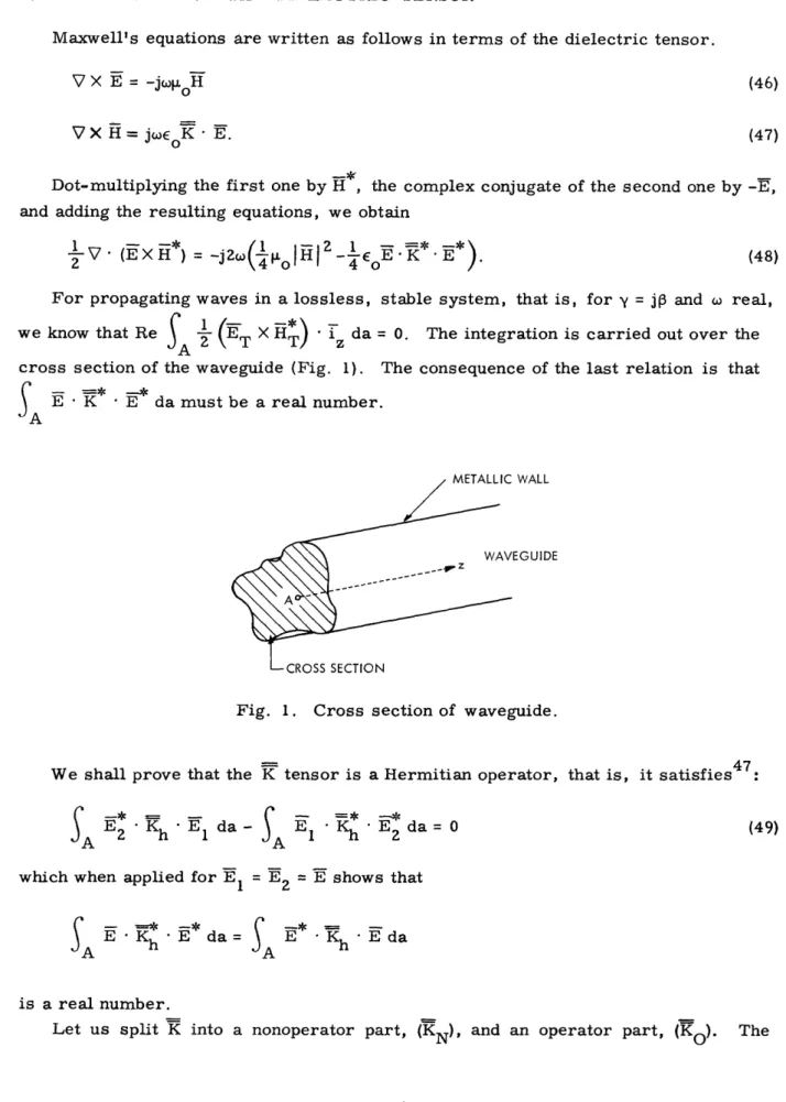
we know that Re A (ET X H) iz da = 0. The integration is carried out over the

cross section of the waveguide (Fig. 1). The consequence of the last relation is that

A

VWALL

EGUIDE

Fig. 1. Cross section of waveguide.

We shall prove that the K tensor is a Hermitian operator, that is, it satisfies4 7:

SA2

S

which when applied for E1 = E2 = E shows that

KE * E da= EKh

Ah A

is a real number.

Let us split K into a nonoperator part, (KN), and an operator part, (Ko). The

16

tensor KN contains the elements KI, Kx, K. The tensor KO contains the differential operators. The coefficients of these operators are K4, K5, K6, and K7.

For a propagating wave, y = jp, all K are real, since w r is real. Therefore the

nonoperator part of the K tensor is obviously Hermitian. For KO, we get

E-* E da- *K O E2 da = j VT (EZ1 E +E*

-A

EZ V _~O - VEl

daE--+ V * k 6 (ElVT z2-EzZ Tzl/j

S TL V K7 VT (EzlEZz) da

When the wall of the waveguide is lossless, Ezl = Ez = 0 on the wall. Applying Gauss' theorem and using the above-mentioned boundary conditions, we find that the right-hand side of the equation above is zero. Therefore Eq. 49 has been proved.

For complex waves y = a + j, in a system which may be described by the tensor (43), this dielectric tensor has both Hermitian and anti-Hermitian parts:

K = Kh + K. The definition for K is

CA

S

In the proof for the Hermitian character of K we used the property that the K are real for y = jp. Therefore when y = a + jp, the tensor Kh will be found when we

consider the real part of K, and the tensor Ka when we consider the imaginary part of K.

2.6 BOUNDARY CONDITIONS

For the derivation of the boundary conditions let us assume a circular cylindrical waveguide of radius a. At radius b (b < a) there is a discontinuity for some species

(vom1 # vom2 and/or Poml * Pom2) We know that the tangential E field and the

normal H field must be continuous at r = b. According to a technique suggested by Hahn,48 we replace the first-order ripple perturbation of the boundary by an equivalent first-order surface charge density (m) and a first-order current density (Czm).

For a rigorous solution the method may be applied only when there is no variation of the electric field in the boundary layer. When the forces on the electrons vary

17

rapidly within the layer, then a scrambling of the electrons takes place, because of the nonsynchronous motions of electrons.3 9 For an unneutralized beam it has been shown that the variation of the electric field in the boundary layer is zero within a first-order

approximation of the transverse displacement vector FT. In a neutral plasma column a sheath is formed around the column. The sheath, of course, is not neutral. For a rigorous solution this sheath must be examined. In the present treatment we assume that the variation of the total electric field at the perturbed position is small.4 9

From the equation

EoV E = p = . Pm (51)

m

we derive the boundary condition

Eo(ErlEr2) =

k

m

From Eq. 21 we derive the second boundary condition:

HO1 - H02 = Czm.(53)

m

In order to derive the boundary conditions with our K-tensor formulation, we need the following equations, as well as (46) and (47),

V' (EoK- E) = 0 (54)

and

V' H = 0. (55)

Equations 46 and 55 yield again the results that the tangential E field and the normal H field are continuous.

For the derivation of the other boundary conditions, we consider a boundary layer of width Ar, which separates part 2 (r < b) of the waveguide from part 1 (b < r). The medium in part 2 is described by a tensor K2 of the form given by (43). The tensor

K1 of the same form, but with different values for its K, describes the medium in part 1. In the boundary layer we assume that each K has a smooth transition from its value at 2 to its value at 1. We do not assume any specific form for this transition,

as long as it is smooth.

If we integrate (47) over the frame bAO, Ar (Fig. 2), we obtain

18

(H01-H0 2) bA = WE0o r r[rj K4 K E + 5E

I

fo

e

Fig. 2. Boundary layer.

As it may be seen from Fig. 2 the "Z" in (56) denotes b - Ar

2' and "1" denotes b + As Ar - 0 the boundary layer degenerates into a sharp boundary and "2" denotes b and "1" denotes b+. Equation 56 yields /W K H _0H1 - H = oE _{EO [(k} K _Er jEoo E 0 i k E o o = WE oX i m

[

_(m

·

where

Wm

The definition of Xm is given by Eqs. 33-38 and Eq. 44. We have property:

used the following

v om X4m o Xlm' rm v om X5m = om Xxm rm v X6m - o X4m' rm v om X7m = X 5m rm 19 ___I_

From Eq. 49 we get by integration over the pillbox Ar, bAO, Az shown in Fig. 2:

K KK

Eo [(K E)rl -(K E)r2] b r rL (Jko E + o

K6 . 7 x

k2 r Ez j k2 r E r

0 0

or

E (E rl-E 2) + (Xm E) r] 0 (58)

Comparing Eqs. 58 and 52, we get

Em

E)rl

= WE 0 [ ](59) rm

From (57) and (53), we find

CZm = WEo _rmm (Xm E)r 1 (60)

As a check we calculate

acr aC V 2

m + zm _ om = -)

az jOEolrm (Xm' E)r + jY orm ( E)

at

z

rm

= Joo[(Xm E) r]1 rm2 rml'

as is expected from the law of conservation of charge applied to the pillbox at the bound-ary.

2.7 WARM PLASMAS

Thus far we have treated cases of temperate plasma. We have used a multispecies theory without any restriction on the number of species and without any restriction on the number of species with initial DC velocity, in order to be able to formulate a theory that may be extended to warm plasmas. We have not elaborated on this extension. Our purpose now is to show how the extension of the theory to warm plasmas may be accom-plished.

We consider the model of a plasma as derived from the Boltzmann transport theory without collisions.5 0 Let f (v ) be the unperturbed one-dimensional velocity

distri-mth ci (Fig. 3). 51

bution function for the m species (Fig. 3).

fom

V_om

Vom,

Fig. 3. Velocity distribution.

A charge p omV = p f(v om) v OmAV, where AV is a volume element, is moving

with velocity vom. We may consider that the m species has been built up of subspecies

of charge density Pom = Om(v Om ) = Pomfom(vom, )6vom. Their plasma

frequen-2 2

cies will be wp =2 f (v )vm In the limit 6v - 0 the summation of the

pm, pm om om, [)om

various subspecies will become an integration over the entire velocity range.

Let us consider a stationary plasma, with a Maxwellian distribution of velocities.

Taking as an example K1 e' where e stands for plasma electrons, we find approximately,

by expansion into series,

2 K z 2 + foe(voe) dvoe pe (61) ,e -Cpe =_0 +v - 2 2 _{2 '} -o yo CO~j + ¥ Vte where 3 ee [Toe (6) v = (62) te i/ me

is the rms thermal velocity, and Toe is the temperature of the plasma electrons in elec-tron volts.

The integration in (61) has been carried out by expansion into series. The result 14

is valid when y vte is much larger or smaller than w. In order to avoid the heavy computational work required for a Maxwellian distribution of velocities we may use a resonant type of curve.52

Analogous procedures can be followed for the rest of the elements of the dielectric

21

tensor. (This is beyond the scope of the present work.) Our intention is to show how our multispecies theory may be extended to study warm plasmas.

2.8 SPECIAL CASES

We have treated a general relativistic case with transverse variation of v and p

om om

(Eq. 43), or without these transverse variations (Eq. 28). Now we shall study the sim-plifications of the dielectric tensor in some special cases.

a. Plane Waves

If we assume a plane wave of the form exp[j(wt-k r)], with k in the x-z plane, the dielectric tensor becomes

k K1 -jKx K4 k O ... k k k x jK * K jK5 kx 0 J5 k .. °... k: k : k K x -jK K l+ 6 kx __ ' o~~~~~~~ (63)

Relation (63) has already been used for the investigation of various waves.53

We notice that in the case of plane waves, when no boundaries are assumed, kx must be a real number for the K tensor to be Hermitian.

b. Infinite Ionic Mass

The ions of the plasma are much heavier than the electrons. Therefore for large 2

frequencies (>>wpiw>>ci) we may assume mi - ° and therefore pi- 0. In this case we omit from the dielectric tensor the influence of a whole species (Xi0).

c. Infinite Magnetostatic Field

The cyclotron frequency of each species becomes extremely large ( cm-oo). Because of the large magnetostatic field we have actually a one-dimensional case (Tm-0). Then

2

o

pzm

K= 1 and K = 1 - 2 The other elements of the dielectric tensor vanish.

m rm

d. Temperate Plasma and Beam

The term "temperate" was introduced by Allis4 1 for the case in which the electron and ion temperatures may be neglected, and a linearization of the Boltzmann equation

is possible. The term "cold" plasma was used for the case of negligible temperatures

22

__ __

l

(vt=O). In this case a linearization of the Boltzmann equation is not possible, since the condition for that is vt >> vin, where vin is the induced velocity of the average particle.

In a rigorous way a temperate plasma is defined as a plasma satisfying the condition Vph >> Vt >> vin' where vph is the phase velocity.

When we neglect the effects of temperature only the beam electrons have DC velocity. We use the subscript b for beam electrons, e for plasma electrons, and i for plasma ions. There are only three species: m = b, e,i. We note that X4m = X5m = X6m = X7m = 0 for the plasma ions and electrons. The elements of the dielectric tensor are

2 pe K = 1 + - Z - W ce 2 pi +2 2 ci -2 2 ( ( ( . pe ce pi ci x =2 e 2 ) + (22) 2 2 2 'pe pi pzb K1 =1 -2 - 2 2 C W W-1 2 K4 WpTbrb k- ₂ 2 r 2 ob 2 k 0 W( cb-rb) Vb K 5 WpTbcb k° Wr (wcb rb bb) 2 K6 WpTb 2 2 2 2 ko Xcub rb 2 K7 'pTb~cb 7_ 2 2- b2 ( 2 o2 \ Vob' ko 0 Wrb" (' cb- Orb ) 2 We note that wcb = ce and wpb

cb wee pb + ~3 + 2 2 °pTb~°rb 2/(oo2 _o2 Z (wcb Srb ) 2 'pTb'cbWrb 2(2 2 a 'cb-~rb) (64) (65) (66) (67) (68) (69) (70) nb 2

=b 2, where nb and n are the densities of beam

ne pe b e

and plasma electrons.

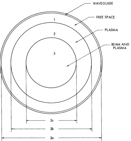
The boundary conditions for a configuration shown in Fig. 4 are

tangential Hnormal = 0.

23

(71)

M AND ,SMA

Fig. 4. Circular waveguide partially filled by beam and plasma.

At r = b (boundary between plasma and free space),

Eo(Erl-Er2) = ( e+u ir=b o[ (X+i) · E]r, 2

HHr, Hz, E, E are continuous.

At r = c (boundary between plasma and beam + plasma), E0 (Er2-Er3) = (b+ e+ i) lr= c

where

0 (X- E)

Wrb b )r,3

blr=c

(e+i) r= c o {t(Xe+Xi) Er,3

(77) HO2 - H0 3 = vb'b r= 24 (72) (73) and (74) (75) (76) ___ ~AIA/Cr-lln x Xi Ke+=)'TE1rzI

e. Nonrelativistic DC Velocity

~ 2 2 2

Assuming that v << c, we get R 1 and therefore = 2 = cm =

om om pTm pzm pm cm

e

m Tm = 1zm M

m

Other simplifications can be applied for the extremely important case of slow waves (vph<<c). The quasi-static approximation (VXEO0) is also very important. These cases will be examined in Section III.

25

III. FIELD ANALYSIS AND CONSERVATION PRINCIPLES

3. 1 INTRODUCTION

a. Field Analysis

We know that for a linear system with uniformity in the z-direction the solutions of the electromagnetic fields have a z-dependence of the form exp(-yz). The time depend-ence is given by exp(jwt), where o is the radian frequency which is assumed to be real. The longitudinal wave number y is independent of position, but it does depend on the fre-quency, the density of each species, and the magnetostatic field. The relation between y and (dispersion relation) may be found from Maxwell's equations and the Lorentz force equation. Since we are interested in the dispersion relation and the electromag-netic fields, we shall use the following procedure. We shall first complete the study of the fields, and then by use of these results we shall obtain the dispersion relation.

There are many approaches to the field analysis. We shall choose an analysis

sim-28

ilar to the normal-mode expansion in isotropic waveguides. Suhl and Walker were the first to show that for a circular waveguide filled by ferrite both electric and magnetic longitudinal fields are nonzero. Kales considered waveguides of arbitrary cross section containing gyromagnetic media, and he derived results concerning wave propagation in these waveguides. 9 The same results as those of Suhl and Walker were obtained by Gamo,3 0 who gave a detailed analysis of the circular waveguide filled by ferrite. Van Trier examined the corresponding problem for a rectangular waveguide.31 He also gave the first complete analysis of guided waves in anisotropic media.32 A very thorough analysis of guided waves in plasma has been given by Bers.3 3

We use the following procedure here. We separate the field vectors into transverse (T) and longitudinal (z) components. We make use of the Maxwell's equations written in terms of the K tensor. We have already used the Lorentz force equation for the der-ivation of the K tensor. By manipulations of Maxwell's equations we find the partial differential equations governing the longitudinal electric and magnetic fields. We derive the dispersion relations relating the transverse fields to the longitudinal fields. Then we proceed to the field solution and derive the dispersion relation by use of the partial

dif-ferential equations for the longitudinal fields.

In Appendix A we examine the case of an electron beam as an example of the general theory given in sections 3. 2-3.4. By use of this theory we may find the field solution and the dispersion equation.

The expression for the longitudinal wave number is extremely complicated. Simpler equations can be found for the critical frequencies, that is, cutoffs (y-0) and resonances in propagation (¥-coo). These resonances in propagation are extreme cases of the more general and very useful range of slow waves (vph<<C). The simplifications that can be made for the special cases will be examined.

A very important approximation for the analysis of guided waves in anisotropic media is the quasi-static approximation introduced by Smullin and Chorney2 0 and Gould and

Trivelpiece. 1 We extend this approximative method to the beam-plasma system and we examine the region of its validity.

Finally, by use of the fields already found we must satisfy the boundary conditions. This procedure yields the so-called determinantal equations. The derivation of the determinantal equations for the specific geometries of a waveguide consisting of two parallel plates and of a circular waveguide is given in Appendix B. The simultaneous solution of the dispersion and determinantal equations yields the longitudinal number as a function of the frequency and the parameters of the system.

b. Conservation Principles

We have analyzed the beam-plasma system by use of the small-signal theory. That is, we have used a linearized system of equations. In analogy with the procedure intro-duced by L. J. Chu3 5 we may derive conservation principles for this linearized sys-tem.54 The quantities introduced in these theorems are products of first-order quantities of the system, and are conveniently interpreted as small-signal power and energy. Although their instantaneous expressions are not unique, the time average of the small-signal power (for real frequency) integrated over the cross section of the

wave-guide and the time average of the small-signal energy per unit length (for real frequency and propagating waves y = j) integrated over the cross section of the waveguide are unique. 19,9 The usefulness of these quantities is well established.19

Since we have used two kinds of descriptions for the beam-plasma system, that is, one by use of mechanical and electrical variables and another by use of the K tensor and

electrical variables only, we may classify the conservation principles into two corre-sponding types.

Among the conservation principles making use of the mechanical and electrical vari-ables, the first one was formulated by L. J. Chu,35 in 1951, for the case of a nonrela-tivistic electron beam in an infinite magnetostatic field. Later Haus and Bobroff3 6

derived the power terms for a nonrelativistic filamentary beam in a finite magnetostatic field. Then Sturrock formulated a variational principle and an energy theorem for non-relativistic beams and plasmas by use of electromagnetic potentials. 37 Bers and Penfield derived the power and energy terms for an irrotational relativistic beam. 8 Bers also formulated a conservation principle for warm plasmas. 55Bobroff, Haus, and Kliiver3 9 have generalized their previous theorem to nonrelativistic beam in arbitrary field.

Kliiver has also given a formulation of the same based on electromagnetic potentials.4 0 A bidirectional waveguide theorem that is due to Chorney56 relates the real and imag-inary parts of the longitudinal wave number to the energy and power terms of the system. This theorem was derived by Chorney for bidirectional waveguides from a consideration of standing waves. Bers and Penfield,5 7 by means of a new technique that does not require standing waves, derived the logical extension for nonbidirectional systems with the restriction that each species of the system be irrotational. This is the same restric-tion that was applied for the derivarestric-tion of their power theorem.38 A generalizarestric-tion for

27

the case of a rotational, unidirectional, and rectilinear beam has been accomplished.54 For the conservation principles that make use of the K tensor and electrical variables only the first theorems were introduced by Chorney56 for a bidirectional plasma system. Bers and Penfield generalized these results by a new approach for a unidirectional but irrotational beam,56 and unidirectional plasma.57 In this report we generalize for the case of a rotational unidirectional and rectilinear beam.

Finally, we include variational theorems and applications for the beam-plasma sys-tem. Bers has given the variational theorems and principles for plasma.5 8

Throughout Section III we assume that the system is homogeneous.

3.2 RELATIONS BETWEEN THE LONGITUDINAL FIELDS

From the divergence equation for the electric field,

V ( K.E) = 0,

we get explicitly

K k )VT T x o ) z (VTX T)

+ j 26VTE z- YK E = 0.

Introducing the following equation derived from Maxwell's equations

iz (VT X ET) = -jCtoHz,

we find

J=YK4 _{( k T + k} jYK6E - H yKEz 0.

2 x z K - E

(78) In order to get the relation between the longitudinal fields, we must express VT ET in Eq. 78 in terms of the longitudinal fields. For this purpose we split Eqs. 46 and 47 into their transverse and longitudinal components::

z V T X ET = -jcoHz (79)

iz X (V X E) = VTE + yE T -j Z X H (80)

iz VT X HT = jCEo(K E)z (81)

i X (VXH) = VTH + YHT = jEoiZ X (K E)T. (82)

Taking the transverse divergence of both sides of (80) and solving for VT ET,

28

VT 'ET =

(K6-1) V2 E - kKIIE + jko K 5 Z

y + jkoK4

An analogous procedure with the use of (82) gives

V H + (kKI+ y2) H VT' ET = k5 o w K x

Substitution of VT · ET as given by Eq. 83

VTEz + aE = bH , where in Eq. 78 yields (85) Kj(Kjk+Y2 ) 2yK4 K1- k o (86) ¥ZK 2 + K4 K k2 6 0 YKs k 2 + ko(KK5-KxK+ 4) 2yK4 K1-j k (87) K6 +__{K -K} 0

Substitution of VT ET as given by Eq. 84 in Eq. 78 and elimination of VTEZ by use of Eq. 85 yields 2 VTHZ + cH = dE, (88) where

/'

I 4

-~~~~~~~~~~~~~~~~~~~~~~~~~~~~~----where b is given by (87).

For plasma alone K4 = K = K6 = 0. Then the coefficients a, b, c, d reduce to the expressions given for plasma by Bers.

For a single electron beam K4, K5 and K6 are, of course, nonzero. Several sim-plifications can be made in the expressions for a, b, c, d. The final expression obtained in this can also be found by examination of the beam in a frame moving with the DC veloc-ity of the beam and by transformation back into the rest frame. The example of the single electron beam is carried out in Appendix A.

The solution of the partial differential equations (85) and (88) gives the expression for Ez and H . For the completion of the field analysis we must find the relation of the transverse fields to the longitudinal fields.

3.3 TRANSVERSE FIELDS

Following the corresponding procedure for plasma by Bers,3 3 _{we get from Eqs. 80} and 82 -Y 0 0 jw w K -Y jWEoK1 0 0 j4L o -Y 0 -joE0oKL 0 o oK -Y ET HT iz X ET i XH_Z T_T 1 0 0 0 K5 K -o k 1 WEO k 0 -j _O o~ o O O 0 1 0 K4 K W4 0 -jWE 1 -0 k0 o ° 0jw6 k0o VTEz VTHz iz X VTE iZ X VTHZ

Inverting the first matrix of (91), we get

p r q s t p u q -q -s p r -u -q t p 1 0 0 0 K K -jwE k 1 WE k 0 0 0 0 0 1 0 K4 K -WE 0 jwE k - o₀ O0 (92) 30 ET iT iz X ET z X HT (91) VTEz VTHz iz X VTEz i XVH z VTHz _ _ I

.

Here, = -y(y2+koK)/D (93) r = -'>ok2K /D (94) q = jykoKx/D (95) s= j 0(y 2+koK )/D (96) t = -Eoy 2K/D (97) u t-joKn +kO(-K2X (98) D = (y2 +koKL) 2 (koKx) 2 (99)

Equation (92) can be written as follows:

ET HT zX ET _z HT P r Q s T p U q -Q -s P r -U -q T p VTEz VTHz i X VTEz z X VTHz

(100)

The coefficients P, Q, T, U are explicitly

(y2+k 2K)+jk (K K KK K)+jko 2 K

P - _D (105)

31

I

-[koY K x- Y K5- j ko 2(KLK S-Kx K4)] Q= ko D (106)

WE 'Y'[k

jy

(K±Ks-KxK

jWE₀ [k0y 2K+K_ (3KI-K

)_jy3K

U= (4_xK) D0 (108)

k D

o

These relations complete the field analysis. The procedure for the solution is as follows. First, we find the general solution for the longitudinal fields (Eqs. 85 and 88). From these equations the dispersion equation may be obtained. The transverse fields can be found from the longitudinal fields by use of Eq. 100. These three steps are the subject of the section 3. 4. Finally, we use the field solution to satisfy the boundary con-ditions. This procedure yields the determinantal equations for the boundary conditions. In Appendix B we find the determinantal equations for the specific geometries of two parallel plates and of a circular waveguide. The simultaneous solution of the dispersion and the determinantal equations gives the longitudinal wave number as a function of the frequency and the parameters of the system.

3.4 FIELD SOLUTION AND DISPERSION RELATION

We have proved that a formulation similar to one obtained for plasma alone3 3 can be used for the beam-plasma system. Therefore we may apply to the beam-plasma system the techniques for the field solution and the formulation of the dispersion relation for a plasma.3 3

At first we transform the coupled set of second-order equations (85) and (88) to an uncoupled set of fourth-order equations.

[Vt+(a+c)V+(ac-bd)] [z] = 0 (109)

or equivalently

p)( [T+P2 0 (110)

as it has been proved for a plasma system.

The transverse wave numbers P1 and P2 are the solutions of the dispersion equation

p4 - (a+c)p2 + (ac-bd) = 0. (111)

The general solution of (111) as given by Van Trier3 2 is

E = EZ1 +E _{z zl z2}. (112)

The components of Ez satisfy the simple wave equations:

(VT+P 2) Ezl = 0. (113)

The longitudinal magnetic field is

Hz = hlEzl + hEzz' (114) where 2 2 2 a-p 2 d P2 1 -c d h _1,2 = _b ' - - ₂ ' _b .. ₂ - .. (115) c- 1 ,2 P2, 1 -a

Substitution of (112) and (114) in Eq. 100 yields for the transverse fields

ET HT iz ET i X HT p ra r sa s b - q+- -w pa p qa q T+ - - U+ -b - b Usb ra r (Q+ b ) +b b b brb / qa\ q pa p - b + T+ b VT /T2 Ez1 + Ez2 zX VT 2-p i XV_{2z2 'T} (116)

For plasma alone P = p, Q = q, T = t, U = u and (116) reduces to the expressions given for plasma.6 0

Taking into consideration the complexity of the coefficients a, b, c, d, the results just obtained are complicated. Simplifications can be made for the critical frequencies, cutoffs (y-O), resonances in propagation (y-oo), and also for the slow waves (vph<<c) that are very important for practical applications. The modifications for the critical fre-quencies and the slow waves are examined below.

33

_ _ _ _

3.5 CRITICAL FREQUENCIES AND SLOW WAVES

a. Cutoffs

At cutoffs the longitudinal wave number is zero: y = 0. Since rb = + jyVob' we conclude that w = Wrb' Equations 33-38 show that y is introduced into the elements of the K tensor only through wrb' Therefore the substitution wrb = w in Eqs. 33-38 gives the elements of the dielectric tensor when y = 0. The dielectric tensor remains an oper-ator.

The coefficients a, b, c, d entering into the equations governing the longitudinal fields (Eqs. 85 and 88) and the dispersion relation (111) are given by the following equations for

y= 0: KK I Ik a 2 (117) K +K 42 K K6 jwtoko(K Ks-K K4 b : 5 x 4 (118) K +K 4 -KK 2 K5 1 - K K2 - K6 + 2K4 K c = k2K k2K2 x (119) o ox 2- K K ~~o4 16 d = - -Klb. (120)

For a plasma waveguide K4 = K5 = K6 = 0, and therefore b = d = 0. The longitudinal electric and magnetic fields become uncoupled and we get E and H waves with one trans-verse wave number in each case.6 1 For the beam-plasma system bd • 0, and therefore the longitudinal fields are coupled even at cutoffs. The dispersion equation gives two transverse wave numbers. For the field solution at cutoffs the procedure described in sections 3. 2 and 3. 3 must be followed. Finally, the simultaneous solution of the disper-sion equation and the determinantal equations for the boundary conditions for y = 0 give the cutoff frequencies as a function of the plasma parameters.

b. Slow Waves

For slow waves

I[y

34

KII(Klk K4 2 K6 0o k ( jyKK K - jy-- _{o k} 6 2 K4 Y¥K6 o Y2 2 k2 c=y +kKI o - 2 xk _°

K

J~KSK

The wave equations (85) and (88) are coupled. The dispersion equation (111) gives two transverse wave numbers. For the field solution we must follow the procedure out-lined in sections 3. 2 and 3. 3. An extreme case of slow waves is the resonances in prop-agation, -y -co.

c. Resonances in Propagation

Since

ly

K4 2 K6

1

Equations 125 and 126 are easily derived by using the expressions for the elements of the dielectric tensor, Eqs. 33-38.

The results obtained for the coefficients a, b, c, d are

35

(121)

(122)