Analysis of blade-mounted servoflap actuation for active helicopter rotor control

Analysis of

Blade-Mounted Servoflap Actuation

for Active Helicopter Rotor Control

Masahiko Kuzume Ikuta

Submitted to the Department of Aeronautics and Astronautics in partial fulfillment of the requirements

for the degree of

Master of Science in Aeronautics and Astronautics

Massachusetts Institute of Technology

Copyright

@

The author hereby grants to MIT permission to reproduce and to distribute publicly paper and electronic copies of this thesis document in whole or in part.

Author _

Department of Aeronautics and Astronautics _ Agust 23, 1995 Certified by.

Professor Steven R. Hall Department of Aernautics and Astronautics Thesis Supervisor

/Professor Harold Y. Wachman Chairman, Departmental Graduate Committee

SEP 25 1995

LIBRARIES Accepted by

LIASSACHUSETTS INSTITUTE OF TECHNOLOGY

Analysis of

Blade-Mounted Servoflap Actuation

for Active Helicopter Rotor Control

by

Masahiko Kuzume Ikuta

Submitted to the Department of Aeronautics and Astronautics on August 23, 1995, in partial fulfillment of the

requirements for the degree of

Master of Science in Aeronautics and Astronautics

Abstract

In this thesis, the feasibility of using blade-mounted servoflap actuation or conven-tional root pitch (swashplate) actuation to control helicopter vibration is investigated. A linear, time invariant, state space model is derived and presented in a form of fre-quency response (Bode plot) which is useful for control studies. Multi-blade coordi-nates are used to transform the blade's degrees of freedom in the rotating frame to the rotor disk modes in the non-rotating frame in order to achieve linear, time invariant system. The linearized model provides general trends of the rotor blade behavior at

different flight situations but may not be as accurate at high advance ratio cases. The model was used to investigate the feasibility of using the servoflap actuation on a one-sixth scale CH-47 model rotor. It is found from the model that as little as 3 deg of servoflap deflection can achieve significant level of vibration reduction. Surprisingly, it is also found that an inboard actuator (f = 0.6-0.8) is more effective than an outboard actuator (f = 0.8-1.0). The root pitch actuation is found to be less effective than the servoflap actuation, due to a zero introduced in the transfer function at the frequency of interest.

Thesis Supervisor: Steven R. Hall, Sc.D.

Acknowledgements

There are many people here at MIT to whom I owe my gratitude for giving freely of their time throughout this project. First of all, I would like to thank my advisor, Professor Steven Hall, for his guidance and support. Boeing Helicpters provided data on the model scale version of the CH-47 rotor, as well as simulation data. I would particulary like to thank Leo Dadone, Bob Derham, and Doug Weems of Boeing Helicopters. Their assistance is greatly appreciated.

I also would like to thank Eric Prechtl, Kyle Yang, and James Garcia for the countless help they provided to answer all my questions. In addition, I would like to acknowledge Dr. BooHo Yang for tutoring me in the fundamentals of control theory and providing me his moral support. I am indebted to all my friends in MIT who made these last two years unforgetable.

Lastly, I would like to thank my brothers, Hirotsugu and Akiyoshi Kuzume, my grandparents, Shun-Ichi and Shizue Ikuta, and off course my parents, Katsuhiko and Hisako Kuzume, for everthing.

Contents

1 Introduction

1.1 Root Pitch Actuation ... 1.2 Blade-Mounted Actuation ... 1.3 Thesis Goal and Overview ...

2 Model Derivation

2.1 Rotor Coordinates ... 2.2 M ulti-Blade Coordinates ... 2.3 Finite Element Analysis ... 2.4 Aerodynamic M odel ...

2.5 Inflow Dynam ics . .. .. .. .. . .... ... . . . .. .. . .. . . 2.6 H ub R eactions . . . . 2.7 State Space M odel ...

3 Results and Analysis

3.1 Input and Output Definitions . . . . 3.2 Model Verification ...

3.3 Parametric Studies ...

3.3.1 Forward Flight Velocity Study 3.3.2 Servoflap Location Study... 3.3.3 Blade Tip Motion Comparison

4 Conclusions 17 18 19 20 23 23 24 25 32 37 38 41 45 . . . . . 4 5 . . . . 4 6 . . . . 53 . . . . . 5 3 . . . . 5 7 . . . . . 5 9 63

4.1 Summary of Parametric Studies ... . . .. . . . . 63

4.2 Future Possible Work ... . ... .. 65

A Rotor Integrals and Matrices 67 A.1 Aerodynamic Integrals ... ... ... .. 67

A.2 Structural Integrals ... ... ... ... 68

A.3 A and I M atrices ... 68

A.4 L and M M atrices ... 69

A .5 F M atrices . . . .. . 69

A.6 1 Matrices ... ... ... 70

B Multi-Blade Coordinates 71

C Inflow Dynamics 77

D Listing of Matlab Code 81

List of Figures

2-1 Helicopter Rotor Coordinates ... . . . . . 24

2-2 Blade Sectional Coordinate ... 25

2-3 Finite element example ... .. ... 27

2-4 Assembly process ... 29

2-5 Nondimensional velocities . . . . 34

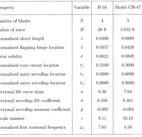
3-1 Blade tip twist angle due to (a) root pitch actuation and (b) servoflap actuation. . . . .. 48

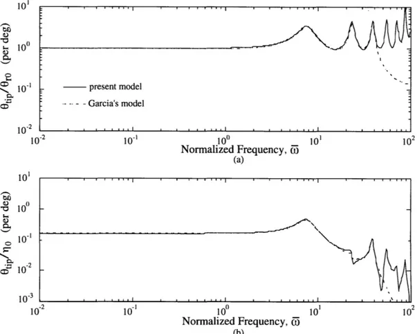
3-2 Goo (jo) by the present model with H-34 rotor blade at various forward speeds . . . .. . . . .. . . . . . ... . 49

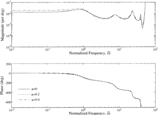
3-3 Goo (jC) by Garcia's model with H-34 rotor blade at various forward sp eeds . . . . . . . . 50

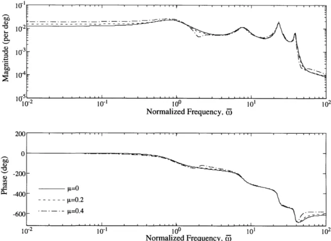
3-4 G,7o(j-) by the state space model with H-34 rotor blade at various forward speeds ... 51

3-5 G,7o(jw) by Garcia's model with H-34 rotor blade at various forward speeds ... . .. ... ... ... ... .. 52

3-6 Go9 o (jo) of model CH-47 rotor at various forward speeds... 54

3-7 GRo(j) of model CH-47 rotor at various forward speeds ... . 55

3-8 The second and third flapping mode shape of model CH-47 rotor blade. 56 3-9 Go (jC) of model CH-47 rotor blade at hover with various servoflap locations. . . . .. . . . . . .. . . . 57

3-10 G,1(jC) of model CH-47 rotor blade at p = 0.2 with various servoflap locations. . .. . .. . . . . .. .. .. . . ... . . . . .. . . . . 59

3-11 Rotor blade tip pitch angle verses azimuthal angle at (a) 80 knots and (b) 160 knots. Solid line is the state space model result and dashed line is Boeing's result. ... ... 60 3-12 Coefficient of Lift at blade tip verses azimuthal angle at (a) 80 knots(p =

0.18) and (b) 160 knots(j = 0.36). Solid line is the state space model result and dashed line is Boeing's result. . ... 61

List of Tables

3.1 Baseline Parameters for H-34 and model CH-47 rotors ...

4.1 Effectiveness of root pitch and servoflap actuation at 3/rev for various flight speed and servoflap locations ...

Notation

An attempt was made to use notation as consistent as possible with that of Johnson [11] and Garcia [7]. Dimensionless quantities are normalized by the rotor radius R, the rotation rate , and/or the air density p, where possible.

a blade section lift-curve slope cl0

a modal amplitude of the generalized mode A rotor area, rR 2

A state matrix

Ak rotor integral, see Appendix A B state control matrix

Bk rotor integral, see Appendix A c blade chord

c normalized blade chord, c/R

C output matrix

CL roll moment coefficient, Mx/pAR(QR)2 CM pitch moment coefficient, My/pAR(QR)2

CT thrust coefficient, T/pA(QR)2

Cr/a blade loading

Ck rotor integral, see Appendix A

D output control matrix

Dk rotor integral, see Appendix A e flap hinge offset

e normalized flap hinge offset, e/R Ek rotor integral, see Appendix A El flapping stiffness

Fk rotor integral, see Appendix A GOro _{transfer function, (CT/ a)/Oro}

G,7 transfer function, (CT/a)/ro GJ torsional stiffness

Gk rotor integral, see Appendix A

hi spanwise length of the i th finite element Hk rotor integral, see Appendix A

I identity matrix

Icg blade sectional inertia

jk rotor integral, see Appendix A K blade stiffness matrix in general

ko stiffness of rotor pitch link Kk rotor integral, see Appendix A

f sectional lift force

L aerodynamic matrices, see Appendix A 1C stiffness matrix for inflow dynamics

Lk rotor integral, see Appendix A m blade sectional mass

m sectional moment force M blade mass matrix in general

M aerodynamic matrices, see Appendix A m* rotor integral, see Appendix A

m rotor integral, see Appendix A Mk rotor integral, see Appendix A

M mass matrix for inflow dynamics n _{lift coefficient of servoflap, cl,}

ii normalized lift coefficient of servoflap, cl,/a N number of blades

Ne number of elements in finite element model nm number of modes selected for generalized purpose

p _{moment coefficient of servoflap, cm,}

p1 normalized moment coefficient of servoflap, cm,/a

q blade index

qk eigenvector corresponding to the kth eigenvalue

Q

r2 outboard servoflap location rC root cutout

R rotor radius s Laplace variable

s normalized Laplace variable, s/Q Sk rotor integral, see Appendix A

t time

T tension due to centripetal force T* kinetic coenergy of the rotor blade

u control input vector

u state vector for finite element analysis

up velocity ratio of blade section, normal to disk plane

UR velocity ratio of blade section, in radial direction

UT velocity ratio of blade section, parallel to disk plane U section resultant velocity ratio, u} + u2

V potential energy of the rotor blade w spanwise deflection

x rotating blade chordwise coordinate x normalized chordwise coordinate, x/c

xcg center of gravity offset, positive aft of quarter chord x state vector

y output vector

a blade section angle of attack

ad rotor disk angle with respect to helicopter velocity

0i flapping slope of the i th element, positive upward y Lock number, pacR4/Ib

F aerodynamic hub reaction matrices, see Appendix A A dynamic matrices, see Appendix A

rl servoflap angle

0 blade sectional pitch angle

o8 blade root pitch angle A rotor inflow ratio, Af + Ai

Af free stream inflow ratio, (V sin ad + v)/ QR Ai induced inflow ratio, v/QR

p rotor advance ratio, V cos ad/QR

p air density

a rotor solidity Nc/7R

me Wk Wk S Subscripts 0 c f i r s Superscripts n T collective longitudinal cyclic free stream induced flow blade root lateral cyclic derivative

exponent on r, see Appendix A transpose

mth flapping deflection mode shape m th flapping slope mode shape m th torsional mode shape rigid twisting mode shape

eigenvector matrix used for generalizing purpose inertial hub reaction matrices, see Appendix A azimuth angle of rotor blade

azimuth angle of q th rotor blade dynamic matrices, see Appendix A frequency [rad/s]

nondimensional frequency w/1

natural frequency of k th generalized mode

normalized natural frequency of k th generalized mode, wk/Q

Chapter 1

Introduction

Helicopter rotors are subjected to periodic aerodynamic forces, especially due to so-called blade vortex interaction (BVI). BVI can cause significant levels of vibration, which reduces pilot effectiveness, passenger comfort, and increases structural weight and maintenance cost. Therefore, reducing vibration is of great interest.

The main cause of BVI is the blade tip vortices created by the spinning rotor. As the rotor spins, these vortices trail and create a nonuniform flow field behind each blade, and the passage of the other blades through the nonuniform flow field causes them to vibrate. As each blade moves around the azimuth, it experiences aerodynamic forcing. The forcing is periodic, so that the blade experiences the same force each time it passes a given azimuthal position. Therefore, the force on each blade can be Fourier decomposed as a sum of sines and cosines, with frequencies at integer multiples of the rotation rate, Q. The forces experienced by one blade will be the same as the forces experienced by another, except for a change in the phase. When summing up the forces from all the blades, the phase differences cause the forces to cancel, except at multiples of the blade passage frequency, NQ, where N is the number of blades. Controlling these harmonics is known as higher harmonic control (HHC). Much research effort has been directed to the use of HHC theory, and number of wind-tunnel tests, as well as flight tests, were performed based on the HHC algorithms [19] [22]. For more complete references to HHC techniques, see

There are several ways to reduce vibrations, including the use of a rotor isolation system [3], a floor/fuel isolation system [4], and vibration absorbers [10]. In this thesis, we are concerned with using the rotor itself to control vibrations. There are two ways to actuate the rotor. Most of the HHC literature has assumed root pitch actuation through the swashplate. The other approach is to use some sort of blade-mounted actuation. These two methods are discussed in the sections below.

1.1

Root Pitch Actuation

Conventional helicopter rotors are controlled by a swashplate, located below the hub of the main rotor, which converts pilot controls in the fixed frame to blade pitch angle in the rotating frame. By moving the swashplate through the flight control, the pilot can control the collective thrust, the pitching moment, and the rolling moment of the helicopter rotor. Shaw et al. [19] have demonstrated the use of closed-loop HHC on a dynamically scaled model of the three-bladed CH-47D rotor. The controller applied small amounts of oscillatory swashplate motion to produce multi-harmonic blade pitch angle of up to +3.0 degrees, and they were able to demonstrate a 90 percent decrease in vibratory shears at the hub. Kottapalli et al. [12] have showed similar results using a 4 bladed full scale S-76 rotor.

There are two problems with the use of the swashplate for rotor control. First, in order to achieve HHC, the swashplate must be actuated as fast as NQ, where a typical value of Q is 200 RPM. Therefore, actuation must take place at about 10 Hz, and accomplishing that with a swashplate is difficult. Second, the swashplate has only three degrees of freedom. For some applications other than HHC (blade tracking, noise control etc) it is desirable to control each blade individually. It is not possible to control the blades of a rotor with four or more blades individually using only a swashplate.

In order to resolve the problem of the limited degrees of freedom, the conventional swashplate actuation can be substituted with servo actuators for each blade. Use of such actuators makes it possible to apply individual control to any number of rotor

blades. This control strategy is called individual blade control (IBC).

Jacklin and Nguyen[16] have demonstrated the IBC technique on a full scale BO-105 rotor by replacing the rotating pitchlinks at the hub with servo actuators. The effect of up to

+1.2

One difficulty with direct control of blade root pitch is the weight and complexity of the actuators. Generally, the power density of electric actuators is too low. Hydraulic actuators have higher power densities, but it is impractical to use hydraulics in the rotating frame.

1.2

Blade-Mounted Actuation

Blade-mounted actuation have been developed as another vibration reduction method. The blade-mounted methods include the use of circulation control rotor (CCR) [21] and servoflap control [20] method.

CCR is based on the Coanda Effect, in which tangential air flow from the trail-ing edge of an elliptically shaped rotor blade delays the boundary layer separation, providing high sectional lift coefficients. HHC can be achieved without moving any parts except the rotating blade itself. However, the mechanical complexity of CCR limits its usage.

Mounting an actuator on a helicopter blade for HHC is not an easy task, due to the limited space within or around each blade and the large centripetal force exerted during normal operations. A helicopter blade is a long thin structure usually built with solid shell and honeycomb fillings. The available space for placing a servoflap is, therefore, limited. Also, during a normal flight, the rotor blades experience a centripetal force on the order of hundreds of g's. These considerations eliminate the use of any type of conventional hydraulic systems.

Spangler and Hall [20] first suggested the use of active materials to actuate a servoflap for rotor control. They proposed using a piezoelectric bimorph bender to actuate a trailing edge flap. Piezoelectric ceramics possess the high bandwidth

necessary for rotor control. Furthermore, they are solid state devices requiring no additional moving parts for operation. Spangler and Hall demonstrated the bender concept in a wind tunnel by incorporating a dynamically scaled actuator into a one fifth model scale CH-47 rotor blade section. Their results showed that blade-mounted actuation is possible, but they ran into problems due to friction and backlash in the flap hinges.

Hall and Prechtl [8] improved on this design, eliminating the friction and backlash problems by replacing the hinges with flexures. In addition, they increased the bender mechanical efficiency by tapering its cross-sectional properties. They conducted a bench test of this actuator and demonstrated flap deflections of ±11.5 deg under no-load conditions. Their results show that, if properly scaled, this actuator can provide up to ±5 deg of flap deflection at the 90 percent span location of an operational helicopter in hover. Furthermore, the bandwidth of their actuator went as high as 7/rev in the experiment and, with proper inertial scaling, can be raised to 10/rev.

Piezoelectric ceramics, on the other hand, are heavy and brittle material. There-fore, placing them in such an aggressive environment as a helicopter rotor blade requires much thought to ensure actuator lifetimes. It is not clear that a piezoelectric bender is the best way to actuate a trailing edge flap. Current research at MIT is examining a number of actuator alternatives to achieve the same goal.

1.3

Thesis Goal and Overview

Due to the complex dynamics and aeroelasticity involved in helicopter rotor oper-ations, it is necessary to computationally simulate the rotor dynamics in order to investigate the feasibility of adding the active control system. Developing a simple, linear time invariant model of a helicopter rotor would allow us to observe the trends of the rotor behavior at various flying conditions. Fox [6] has developed a linear, time invariant, state space rotor model using multi-blade coordinates to transform dynam-ics from the rotating frame to the fixed frame. Garcia's work [7] was the extension of the work done by Fox [6], and this thesis builds on Garcia's work. The goal of

this thesis is to develop a linear time invariant model which incorporates some blade properties which are known to be important for the rotor dynamics but are excluded in Garcia's model. Such properties include the blade elastic bending properties and the blade spanwise center of gravity offset distribution.

Chapter 2 explains the derivation of the state space model of a rotor system with assumptions such as time invariant rotor dynamics and linear aerodynamic forces. Multi-blade coordinates are used to achieve successful transformation from rotating frame dynamics to non-rotating frame dynamics.

Chapter 3 presents results of the linear, time invariant, state space model derived in Chapter 2. The model is validated by comparing certain results with the results obtained by Garcia's [7] state space model. Parametric studies using a one-sixth model scale CH-47 rotor are done by varying properties such as servofiap spanwise location and helicopter forward velocity. The thrust response due to collective root pitch actuation and servoflap actuation are the primary interest, therefore, thrust frequency response due to such actuations are presented and studied in the form of Bode plots.

Chapter 4 presents the summary of the important conclusions, and some sugges-tions for the possible further research are listed.

Chapter 2

Model Derivation

In this chapter, a linear, time invariant, state space model of a helicopter rotor is developed. A semi-articulated rotor model with elastic flapping and elastic torsion is assumed. The inputs of the state space system are the root pitch angle and servoflap deflection. The outputs are the hub loads, namely, vertical force, pitching moment, and rolling moment. The model is derived by first finding the stiffness and mass matrices of the rotor blade from the blade structural properties using a finite element method. The natural frequencies of the blade flapping and torsion, as well as their mode shapes are simultaneously found. Then, the forces and moments due to aero-dynamic forces due to modal deflections are calculated. Modal forces and moments are then transformed from the rotating frame to the fixed frame using multi-blade coordinates (MBC). A dynamic inflow model developed by Pitt and Peters [17] is also added to the dynamics. Finally, these structural dynamics, aerodynamics and inflow dynamics are coupled together to form a state space model of a helicopter rotor which includes root pitch and servoflap actuations. Before the derivation of the state space model, the notation and coordinates of the rotor system is presented.

2.1

Rotor Coordinates

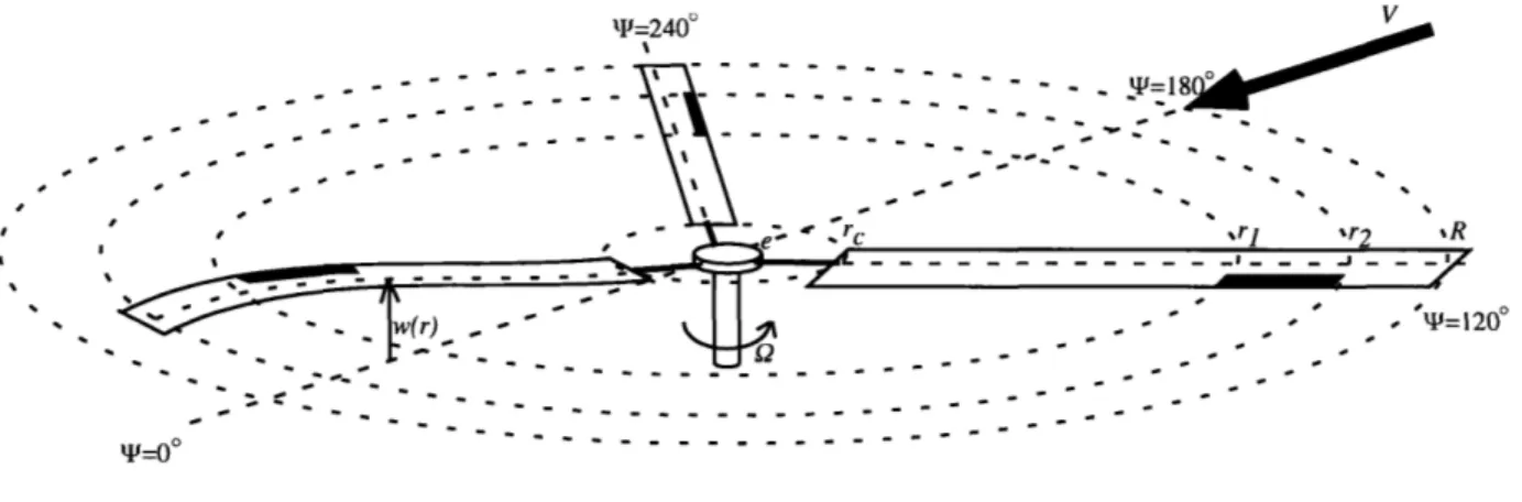
Polar coordinates are used to describe a rotor disk: r for radial position and 0I for azimuth angle. These coordinates are illustrated in Figure 2-1. It is assumed that the

T =2400 --- - -e rc ,rI % r2 r w(r) - " . " " ." p= T= 120 0 q j = -o " . . . .. . . .

Figure 2-1: Helicopter Rotor Coordinates

rotor rotates counterclockwise if viewed from the top, as is conventional for American

helicopters. The rotational velocity is denoted Q. Each blade flaps elastically about a flapping hinge at r = e, and the blade's spanwise flapping displacement from the horizontal plane is denoted w(r). Servoflaps are located between spanwise locations rl and r2 of each blade, and servoflaps are deflected an angle of rl, defined positive downward. Each blade is also allowed to twist elastically across the span with an angle 0, defined nose up positive. In order to achieve root pitch actuation, the whole blade is allowed to pitch rigidly with an angle 0r. For this model, the pitch axis coincides with the neutral axis at the quarter chord. The center of gravity offset is denoted xzg defined aft of quarter chord positive. The sectional coordinate are illustrated in Figure 2-2. For convenience, the normalized radial location is f = r/R

and the normalized chordwise location is t = x/c.

2.2

Multi-Blade Coordinates

In this chapter, a linear, time invariant, state space model is derived. A linear, time invariant system allows the use of frequency response as a method for rotor dynamics simulation. Frequency response has not been thought to suite as a method of solution to rotor blade dynamics simulation because rotor blade dynamic forces are periodic

1/4 C X c

g-Figure 2-2: Blade Sectional Coordinate

and incorporating periodic effects into frequency response is very complicated. In the previous work such as Shaw [19], NQ root pitch actuations were often evaluated in a form of T matrix. T matrix shows the NQ cosine and sine output effects due to NQ cosine and sine input with varying forward speed. The results of the T ma-trix, however, often showed only a small influence of periodic effects in the output. Therefore, by neglecting certain periodic terms, linear, time invariant, system of the rotor blade dynamics could be derived, and the frequency response of both root pitch and servoflap actuations can be obtained. Multi-blade coordinates (MBC) are used to transform blade forcing properties from the rotating frame to the non-rotating frame in order to achieve linear, time invariant, system. In Appendix B, the general procedure of using MBC and an example are given. This information is taken from Garcia [7, chapter 2]. A more detailed explanation is available in Johnson [11].

2.3

Finite Element Analysis

In this section, the finite element procedure used to model the blade's elastic motion is described. The finite element model will produce equations of motion of the form

Mii + Ku = Q (2.1)

where M, and K are the mass and stiffness matrices, respectively, u is a vector of elastic degrees of freedom, and Q is the forcing term from aerodynamics. In this study,

material damping is ignored, and hence there is no damping term in Equation 2.1. All damping in the model will arise from aerodynamic considerations. The objective of the finite element code developed in this section is to find the stiffness and mass matrices of Equation 2.1, and also find the natural frequencies with the corresponding mode shapes for a given rotor blade. The natural frequencies and the mode shapes are obtained by solving the generalized eigenvalue problem

Kqk = W Mqk (2.2)

where wk is the kth natural frequency and qk is the corresponding mode shape. The stiffness and mass matrices can be found by many different techniques. Garcia [7] used a lumped mass model to simulate the blade properties. However, due to the limited number of masses which can be incorporated in a lumped mass model, only the approximated spanwise properties (mass, inertia etc) could be used. The finite element method, on the other hand, can incorporate the blade properties across the span with much higher precision than the lumped mass model since blade properties are usually given in either tabular or graphical format, and are generally piecewise linear. By breaking up a blade into elements appropriately, each element will have all linear properties. Therefore, much more accurate equations of motion can be derived.

The advantage of the finite element method over any other method is that the equations of motion for the system can be derived by first deriving the equations of motion for a typical finite element and then assembling the individual elements' equations of motion to find the over all system's equation of motion.

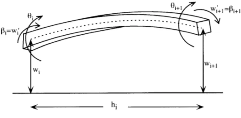
Figure 2-3 shows a typical rotor blade finite element of arbitrary width, hi. Let Ne be the number of total number of blade elements. The motion of the system is defined in terms of the displacement, wi(t), slope, w'(t), and torsional displacement,

Oi, of the element end points, where i varies from 1 to Ne + 1. The stiffness and mass

Figure 2-3: Finite element example

and the kinetic energy, T*, of the element. The potential energy is

1 [h a2W 2 1 hi 2 - hi d 2

V=- EI al dx + - I T dx + - j GJ dx

2 OX2 ) 2o 1X 2Jox

(2.3)

and the kinetic energy is

1 M ( _ xcgo)2

1

T*=

dx

-

Ic2dx

2 o 2 o

(2.4)

where El, T, and GJ in Equation 2.3 are the blade spanwise flapping stiffness, the tension due to blade centripetal force, and the twisting torsional stiffness, respectively. Ig is the blade's sectional moment mass of inertia about its center of gravity. The deflections, w and 0, are interpolated between the element end points via

(2.5) (2.6) where L(x)= Lo(x) - 322 + 2X 3 - 2h. 2 + h,3 322 - 2: 3 -hU 2 + hi 3 (2.7) o(x, t) = L (x) qo (t) w(x, t) = LS

()q(t)

and

Oi

q(t) (q(t) Wi (2.8)

Wi+1 Wi+1

where r = x/hi. The polynomials in L(x) are chosen to satisfy the torsional and bending boundary conditions, which are

I L, (0) Lw2 (0) Lw3 (0) L4 (0) Lo1(0)

-Lo

2(hi)

=

into Equations 2.3 and 2.4, the potential and

1 hi GJ (-9LI ) T 0 V = - q] x dx qo 2 V= 0 E (2) (2 L_ ) T 2 9x2 aX2 49X 09X (2.10)

1

The matrices within each integrals in Equations 2.10 and 2.11 are the stiffness matrix and mass matrix, respectively:

k

ax

)

other

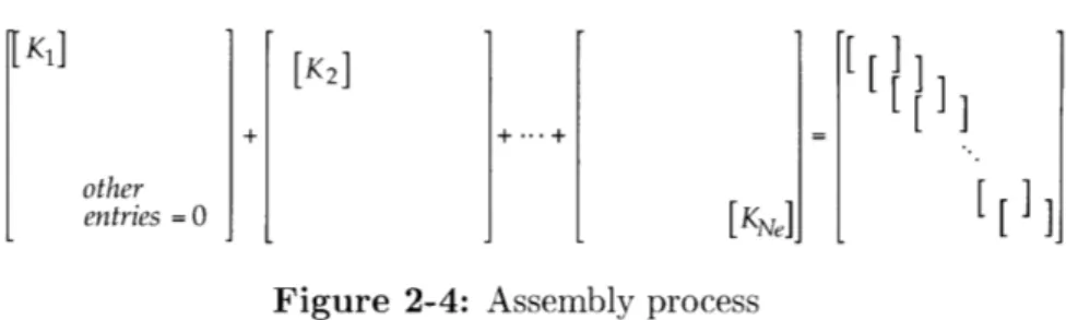
entries = 0 [ KNe]

Figure 2-4: Assembly process

The properties in Equations 2.12 and 2.13 such as GJ, EI, T, m, Ieg, and x, are linear within the element which makes it possible to evaluate the integrals in closed form. The element stiffness and mass matrices are calculated in subroutine FEsubexact .m,

attached in Appendix D.

Each 6 x 6 stiffness and mass matrices represent potential and kinetic energies of each element, and by summing the energies of each element appropriately, the potential and kinetic energies of the whole rotor blade can be found in the form of stiffness and mass matrices. Let Ki and Mi be the stiffness and mass matrices of the

ith element, and K, and M be the stiffness and mass matrices of the whole rotor blade. Then, summing of energies can be accomplished as shown in Figure 2-4. The stiffness matrix of the whole blade, K,, is found by placing the 6 x 6 stiffness matrices from each element diagonally to each other with left upper and/or right lower 3 x 3 part overlapping to the adjacent matrices. The overlapped parts between the two matrices are the potential energies from the same blade location. Therefore, they are simply added entry by entry. The mass matrix of the whole blade is found the same way. Eventually, both K, and M become (3Ne + 3) x (3Ne + 3), large where Ne is

the number of elements used to model the rotor blade.

The boundary conditions for this rotor blade come from the fact that the flapping deflection and the flapping moment at the flapping hinge are both zero. It is sufficient to satisfy only the geometric boundary condition, wl = 0, to achieve an accurate model. Therefore, the row and column corresponding to wl in Kw and Mw are set to zero and deleted. Finally, to find all the natural frequencies, wk, and the corresponding mode shapes, qk, the eigenvalue problem in Equation 2.2 is solved by using the obtained Kw and Mw.

The eigenvalues represent the combined torsional and flapping natural frequencies of the rotor blade. Each eigenvalue has a corresponding eigenvector, and the eigen-vector which contains information of torsional, flapping deflection and flapping slope modes represents the mode shape of the corresponding eigenvalue. Similar to Fourier Series, a motion of a blade can be expressed as a linear combinations of the mode shapes. The coefficient or the amplifying factor for each mode shape is the modal amplitude which is used as the state variable in the state space model derived in this thesis. In Garcia's approach [7], torsional modes and rigid flapping deflection mode were treated separately whereas the present study combines all torsional, flapping deflection and flapping slope modes as just plain modes. One of the advantages of using combined modes is that the necessary number of modal amplitudes for the state space model is much less. Therefore, fewer state variables are needed. Also, modes with coupled torsion and flapping are easily incorporated into the state space model. One of our objectives for this study is to analyze the effect of rotor blade's root pitch actuation, i. e., swashplate control. In order to do this, there is a need to include a torsional mode which represents pure rigid pitch motion, because the mode shapes obtained from the finite element code have boundary conditions which exclude this rigid pitch mode. Let 40 consist of a vector that represents the rigid pitch mode shape, qgo, and let a0o be the modal amplitude of the rigid pitch mode.

The state vector, u, in Equation 2.1, which consists of the modal amplitudes of all of the eigenvectors, can be simplified and reduced to have a desired number of degrees of freedom by retaining a certain number of modes with lowest frequencies. Let Nm be the desired number of degrees of freedom to be contained in the state space model, then, (L consists of the first Nm columns of eigenvectors, qi's, and aL consists of the first Nm modal amplitudes. The simplification can be accomplished by expressing u as

u = Oa (2.14)

where

and

a [ao aL- [a0o a1 a 2 .' aNm ]. (2.16)

Substituting Equation 2.14 into Equation 2.1 and multiplying by IT _{on both sides,}

the equations of motion can be rewritten as

(WTMWn i + T K,(a = DTQ. _(2.17)

Substituting Equation 2.15 and 2.16 into Equation 2.17, the equations of motion can be rewritten as

qo Mqo q0OM.qL

i

i

qLMqo qjM~qL L qj Kwqo q KqL aL q

The matrices above may be simplified as

MOO MOL

do

Koo

KOL

ao

+ = (2.19)

MLO MLL aL KLO KLL aL QL

where subscripts with 0 represents properties of the rigid pitch motion and subscripts with L represents properties of other modes. The terms Qo and QL represent the aerodynamic forcing terms applied on the rigid pitch mode and the other modes, respectively, and they are derived in the next section. Notice that the original mass and stiffness matrices from Equation 2.1 were (3Ne + 2) x (3Ne + 2), but the new

mass and stiffness matrices in Equation 2.19 are shrunk to (Nm + 1) x (Nm + 1).

The second row of Equation 2.19 can be rewritten as

MLLGL + KLLaL = QL - ML0o0 - KLao. (2.20)

The term Koo in Equation 2.19 is the stiffness associated with the blade's rigid pitch motion, and is therefore zero. In fact, Koo is not quite zero, due to propeller moment terms. However, these effects are small, and will be ignored. Since K00oo is zero and the stiffness matrix is positive definite, KLO and KOL must be zero. In the

finite element code, however, the pitch link stiffness is incorporated into the blade properties, modeled as one end of the pitch link attached to the blade and the other attached to the swashplate. The finite element code allows the movement of the blade's rigid pitch actuation but holds the swashplate rigid. This motion results in stretching and compressing the pitch link as the root pitch actuation is done. Therefore, the stiffness associated with the blade's rigid pitch motion without moving the swashplate is not zero. The actual root pitch actuation is achieved by actuating both the blade and the swashplate, therefore, the stiffness of the pitch link does not affect the stiffness associated with the rigid pitch motion. This is why Koo as well as KLO and KOL must all be set to zero.

After setting KLO equal to zero, the modal amplitudes and their time-derivatives in Equation 2.20 are transformed using multi-blade coordinates, and the equations of motion become

AiaL + AAZaL + AaaL = QL - la iio - tO 0% - or, ao. (2.21)

The various A and F matrices are defined in Appendix A. In order to complete the derivation, the aerodynamic forcing term, QL, needs to be evaluated.

2.4

Aerodynamic Model

In this section, aerodynamic forcing term, QL, in Equation 2.21 is derived. Linear aerodynamic forces are assumed by keeping sectional lift curve slope, cl,, sectional servoflap lift coefficient, cl,, and other variables constant spanwise and azimuthally. Torsional aerodynamic damping is also included assuming quasi-steady aerodynamics. Before proceeding with the aerodynamic derivations, nondimensional fixed frame and rotating frame velocity components are explained.

The rotor disk may have an angle of attack, ad, _{relative to the helicopter velocity,}

V. The air velocity relative to the rotor disk can be decomposed into two components, one parallel and one normal to the disk plane. After being nondimensionalized by

the blade tip velocity, QR, the parallel velocity component relative to the rotor disk is the advance ratio, P, defined as

V cos ad (2.22)

QR

The normal component of the air velocity is the inflow, A, which is composed of two

parts,

A = A+ Ai (2.23)

where Af is the inflow due to the free stream velocity, V, defined as

V sin ad

A -=V d (2.24)

QR

and Ai is the induced inflow of the rotor.

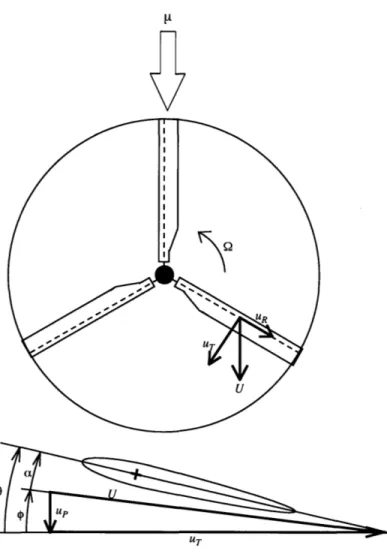
The airflow relative to the blade due to rotor motions can be decomposed into three terms, namely the tangential velocity, UT, defined positive toward trailing edge, radial velocity, uR, defined positive toward blade tip, and normal velocity, up, defined positive up through the disk plane. Figure 2-5 illustrates these velocities, nondimen-sionalized by QR. In forward flight, these velocities are

UT = r + y sin V (2.25)

UR = p cos 4 (2.26)

up = A +t w' cos V + b (2.27)

which are the function of azimuth angle, 4, and radial position, r.

The aerodynamic components that make up the forcing term, QL, in Equation 2.20 are the modal forces due to the airfoil sectional lift and moment. The modal forces are expressed as the sum of the product of a sectional force and the corresponding mode shape over the whole blade. The sectional lift force, with small angle approximation,

Figure 2-5: Nondimensional velocities = -pcuT (QR)2 cl 2 1 = pcu 2 (QR)2 (ac + n) 2 (2.28) (2.29)

where the sectional lift coefficient, c1, is approximated as a linear combination of angle of attack, a, and servoflap deflection angle, r. The sectional lift curve slope, a and

the sectional servoflap lift coefficient, n, are

a = ci (2.30)

n = cl1. (2.31) The sectional moment force is

m = 1pc

~4

where the moment is also assumed to be linear to servoflap deflection, and the sec-tional servoflap moment coefficient, p, is

p = cmq. (2.33)

The airfoil coefficients, a, n, and p are obtained from the 2-dimensional panel code, XFOIL [5], which includes viscous and compressibility effects.

Due to the three-dimensional flow effects, there must be a finite distance near the blade tip to drop blade loading to zero. This so-called tip-loss effect is approximated by assuming the blade loading farther outboard of radial station F = B to be zero. Typical values for B range from 0.96 to 0.98. Therefore, spanwise aerodynamic integrations are carried out from the root cutout, Yf, to B.

The modal force due to lift, L, is obtained by integrating the sectional lift, f, over the corresponding mode shapes. Normalizing L by Ib2 gives

-L -j uoa (r) dr + - u2nr (r) dr (2.34)

where the subscript, m, indicates the mth mode shape. The mth flapping and tor-sional mode shapes are expressed as /j (r) and 00 (r), respectively. The angle of attack, a, can be expressed as

S(r) = r + 0 - (2.35)

= Or + 0- (A + pw' cos + t) . (2.36) UT

Therefore, the modal force can be decomposed into the sum of several terms:

L = Lo, + Lo + LA + Lw, + L, + L₇, (2.37) where , 2U2 OW (2.38) Lorm -2

J

J

LW- = - UTr COS ()O (f) ) d aL (2.41)

2 B

Lm= UT¢ ( ) d f hL, (2.42)

2 Jri

Notice that blade deflection, w, slope, w', and torsional angle, 0 are substituted with the corresponding products of mode shapes and modal amplitudes. Inserting the linear inflow approximation of Equation 2.55, the tangential velocity of Equation 2.25, and the rotor integrals of Appendix A, the modal force components can be rewritten as

Lor = [S2 + 2p sin

oS

Lomn = [Amn + 2p sin OAm + /2 sin2 AO] aL, (2.45)

LAm = - [D' + / sin VD°] \o

-[D2 + tp sin D] (A, cos V + A, sin ) (2.46)

[ ₁₂

= [ cos 2 sin 2 Bmn, aL (2.47)

Lm = n [Cn p sin 'CoC am L (2.48) Lo = [Em + 2p sin VEm + #2 sin2 _V)Eo_]

_m.

The modal force due to moment, M, is obtained by integrating the sectional moment, m, over the corresponding mode shapes. Normalizing M by Ib2 gives

Mm Jp2cu m (f) dr r, - _ 6UTf (f) m (F) df ALm

2 ft 16

rB E2 _{1 02}

- 7 UT (f) Om (f) df ao (2.50)

where the first term, which will be denoted M77m, is the moment modal force on mth

modal shape due to servoflap deflection, and the last two terms, M ₀ and M0 , are the elastic and the root pitch torsional aerodynamic damping terms if quasi-steady aerodynamics are assumed [2]. The term qOr (f) is the mode shape for rigid pitch

motion. Substituting the tangential velocity Equation 2.25, and the rotor integrals of Appendix A, the components of the modal force due to moment can be rewritten as

M = [m [L2 + 2p in L sin _in2Lo] 2 _(2.51)

M6m = [Mm + i sin VM,] aL, (2.52)

Mrm = [Nm + p sin No ] ao0. (2.53) Combining modal forces due to lift and moment and transforming them to MBC, the forcing term, QL, in Equation 2.21 becomes

QL = (La + Ma) aL + (La + M) iL +

(LO, + Mo,) ao + M6 ao + (L, + M,) 7r + LxA (2.54)

where the L and M terms are given in Appendix A.

2.5

Inflow Dynamics

Unlike the fixed wing case, helicopter rotor in forward flight creates very complicated inflow dynamics. The shed wake and trailing vorticities produced by the rotating airfoil creates a skewed helical wake which influences the inflow at the rotor disk, so

that the induced inflow is a complicated function of radius and azimuth. However, a simple linear approximation developed by Pitt and Peters [17] can provide adequate results. The linear inflow approximation

A = A0 + Acf cos + Asf sin (2.55)

is used for the purpose of this research which is based on the actuator disk the-ory. Simple dynamics relate the A perturbations to the aerodynamic loads, namely thrust coefficient, CT, pitch moment coefficient, CM, and roll moment coefficient, CL. Defining the vectors

CT Ao

Yaero- CM , A= Ac , (2.56)

aero

the inflow dynamics presented by Pitt and Peters [17] and used in this research are

A = -M 1_{'C A M-Kyaero}

(2.57)

which can easily be incorporated into the state space model. The inflow dynamics matrices, MA4 and CA, are given in Appendix C.

2.6

Hub Reactions

In the rotating frame, the vertical shear force due to the aerodynamic force minus the inertial force is the applied loading on each blade. These forces can be transformed to non-rotating frame by the MBC transformation, and our nondimensional hub re-actions of interests which are the thrust, pitch moment, and roll moment coefficients,

or CT, CM, and CL, can be found.

The output of interest has two terms,

CT CT CT

CM = CM + CM (2.58)

where the aerodynamic term is the shear force and it is needed to force the inflow dynamics. The vertical shear force at the blade root, S, is the integral of the vertical force acting along the blade. This vertical force is composed of sectional lifting force acting upward and the sectional inertial force acting downward. The resultant forces are normalized by pA (QR)2, and they are

=a B1 -a f2 1 maR R

S =

d +

-

dr

-

-

where angle of attack, c, is defined in Equation 2.36. The vertical shear force may be rewritten as

S= So, + S +SA + S,, +

S+S,+

o, = [F2 + 2/t sin F1 + f2 sin2 Fo] ao (2.61)

2N

= 2

SO =2 [G + 2p sin V)GI _{+ 2} 2 n _{V'Go] a,, (2.62)}

A₌ 2N [F1 + p sin V)Fo] Ao 1

2 [F2 + p sin VF1] (Ac cos + A, sin ) (2.63)

2N

1 1 ₂ ]

S = 2N [ cos pH 2+ f sin 20Hm aLm (2.64)

SM 2 [JA + psinOJm (2.65)

2NS [K2 + 2p sin /)K' + [,2 sin2 ,KO] 7 (2.66)

1 S,- = Mo io (2.67) 1 (2.68) -ian m - Nm*.. aLm (2.68) am N aLma Lm

Summing over N blades, the rotor thrust coefficient is given by

N

T=

(So+

q=

which is equivalent to doing the MBC collective summation operator. mensional moment due to the qth blade is

eS CMq = pAR (QR)2 CMq = E (O, + So+ A + ,S + S + g, + O, + S,). (2.69) The nondi-(2.70) (2.71)

By summing the contributions of all the blades, pitch and roll moment coefficients are CM =

E

which are similar in the form to the MBC cyclic summation operators.

The partial hub reactions due to the aerodynamic effects only and the total hub reactions are CT CM CL _aero CT CM CL

= FaaL + F&aL + FAA + Forao + Fr (2.74)

= (Fr + ~P) aL + (Fr + &) aL + adk

+ (For + oe,) ao + ~,Oro + 4,' ao + FA + Frj (2.75) where the F and 4 matrices are defined in Appendix A.

2.7

State Space Model

Using the dynamic equations of motions defined in Equations 2.21 and 2.54 with the hub reaction Equations 2.74 and 2.75, a linear, time invariant, state space rep-resentation of a rotor with blade-mounted servoflaps can be assembled. The model is

iX = Ax + Bu + Bxyaero, (2.76)

Yaero = CaeroX + DaeroU, (2.77)

y = Cx + Du (2.78)

where the state and control vectors, x and u, are defined as

aL

x= A , u=-. (2.79)

ao

a0

The output vectors, Yaero and y, are defined as

CT CT

Yaero C , Y= C (2.80)

CL _aero Laero

The state space matrices are

0 I 0 0 0

a21 a2 2 a2 3 a2 4 a2 5

A = 0 0 -MjI A-1 0 0 (2.81)

0 0 0 0 I

where a2 1 - A 1 (La + Ma - Aa) a22 - 1= (La + Ma - Aa) a2 3 = A 1L A a2 4 -= A1 (Lo, + Mo - or,) a25 -= 1 (Mo, - o'r) , 0 0 B= 0 0 (2.82) 0 0 I 0 0 0 BA Mj (2.83) 0 0 Caero [Fa Fa FA F, 0] (2.84) Daero =[0 F ] (2.85) C- [c C2 C3 C4 C5 (2.86) where C₁ = Fa + a + aAd1 (La + Ma - "a)

c2 = ra + 4a+

4

C3 FA + 4 1aA-ILA

Or + ~1A 1 (M)

-Ai (L, + M) . (2.87)

Combining Equations 2.76 and 2.77, the dynamic inflow loop can be closed yielding the state space model

x = (A + BACaero)x + (B + BADaero) u,

y = Cx + Du.

(2.88) (2.89)

Chapter 3

Results and Analysis

In this chapter, the notations and definitions of the input and output for the state space model developed in the previous chapter are discussed. Then, the accuracy of the state space model is verified by comparing results with Garcia's results [7]. After validating the model, the behavior of a model scale CH-47 rotor is evaluated by varying parameters such as forward flight speed and servoflap location. The objectives of this parameter studies are to observe the trend of the rotor response to forward flight speed, and estimate the optimal servoflap location

3.1

Input and Output Definitions

In the previous chapter, a linear, time invariant, state space model was developed. The model is capable of simulating both root pitch and servoflap rotor actuations. This model has six inputs, namely collective and two cyclics each for root pitch and servoflap actuations. There are three outputs, namely coefficient of thrust, pitch-ing moment, and rollpitch-ing moment. Hence, the state space model yields 18 individual transfer functions. Of these, we are mainly interested two, the effect of collective root pitch and servoflap actuations on thrust coefficient. The transfer function from

col-lective root pitch to thrust, (CT/cx)/Oro, is denoted by Goro (). Similarly the transfer function from servoflap deflection to thrust is (CTr/)/ro, which is denoted by G,,0 ().

space model, the transfer function for collective root pitch acceleration, (CT/a)/Oro, must be integrated twice, so that

=2 CT/U CT/U

Go, ()= s (3.1)

Oro Oro

The nominal value of CT/a is approximately equivalent to 1 g of thrust, so that

(ACT/a)/(CT/a) is a measure of control authority in g's. For this study, CT/a of

0.1 is assumed, and the control loads required for 0.1 g of higher harmonic control authority is evaluated. The magnitude plots of all Go,0

(o)

In a higher harmonic control system for vibration reduction, the control effort is concentrated around NQ, so for the H-34 rotor the frequencies near 4Q are of interest. Later, for the model CH-47 rotor, the frequencies of interest are near 3Q.

Table 3.1 lists all the baseline parameters for both H-34 rotor blade and model size CH-47 rotor blade used for this analysis. In this study the size of the servoflap is set to 20 percent chord length wide and 20 percent long spanwise. The detailed blade properties are given in the MATLAB input code listed in Appendix D of this thesis.

3.2

Model Verification

As previously stated, the state space model derived in the previous chapter is verified by comparing with Garcia's results [7]. Garcia used Boeing Helicopters' rotor analysis program, C60, for validation of his state space model. In this thesis, some verification of the model was done by comparing it to the model of Garcia. Garcia's model includes torsional bending modes and rigid flapping mode, but does not include any elastic flapping modes. By scaling the flapping stiffness, EI, six orders of magnitude higher from its original value in the present model, a blade with rigid flapping and elastic torsion can be simulated and compared to Garcia's model. In addition, later in this chapter, some results with elastic flapping were compared to simulations run by

Table 3.1: Baseline Parameters for H-34 and model CH-47 rotors

Property Variable H-34 Model CH-47

number of blades N 4 3

radius of rotor R 28 ft 5.052 ft

normalized chord length c 0.0488 0.0889

normalized flapping hinge location 0.0357 0.0420

rotor solidity a 0.0621 0.0849

normalized root cutout location rT 0.2100 0.2000 normalized inner servoflap location i1 0.6000 0.6000 normalized outer servoflap location r2 0.8000 0.8000

sectional lift curve slope a 6.30 7.64

sectional servoflap lift coefficient n 0.500 0.461 sectional servoflap moment coefficient p -0.082 -0.084

Locke number 7 8.11 10.10

normalized first torsional frequency c1 7.65 4.50

Boeing Helicopters, although no systematic verification was done against the Boeing models.

Figure 3-1 shows the frequency response of the blade tip twisting angle due to root pitch actuation and servoflap actuation. The peak around 7.5Q is the first torsional natural frequency, and the next two peaks at higher frequency range are the second and third torsional natural frequencies. Other peaks obtained by the present model but not by Garcia's model are either the higher torsional natural frequencies or the artificially stiffened elastic flapping natural frequencies. The present model (as well as Garcia's model) can incorporate as many torsional modes as needed. For convenience, the present model has nine torsional modes and Garcia's model has three torsional modes. By adding more modes, the accuracy of the frequency response around the

10o S10- - present model - -. - -Garcia's model 1 0 -2 . . . . . . . . . 10-2 10-' 10° 101 102 Normalized Frequency, F (a) 10 1 o 10-a 103I0 103 ., 10-2 10- 10 101 102 Normalized Frequency, 6 (b)

Figure 3-1: Blade tip twist angle due to (a) root pitch actuation and (b) servoflap actuation.

first few modes increases. Therefore, only the results at low frequency range (< 40Q) in Figure 3-1 should be evaluated, and higher frequency range (> 40Q) should be ignored. The level of agreement in the frequency responses of the present model and Garcia's model is quite high in both the root pitch actuation and the servoflap actuation cases.

Figure 3-2 shows the frequency response of Go,o (jC) in edgewise flight at various forward flight velocities using the present model. An advance ratio of 0 corresponds to hover, 0.2 is about 80 nautical knots, and 0.4 is about 160 nautical knots. Notice the magnitude of the root pitch actuation at DC increases slightly as the advance ratio is increased. This is due to the fact that higher advance ratio provides higher dynamic pressure on the advancing side of the rotor, and thus more lift is achieved. It should also be noted that rotor operations at higher advance ratio exhibit greater blade stall effects on the blade retreating side of the rotor. The present model does not include

o 10-2 10 -2 10- 100 101 102 Normalized Frequency, 0) 200 0 ". -200 -400 _{--- [t=0.2} -600 - - - - =0.4 10-2101 100 10' 102 Normalized Frequency, (

Figure 3-2: GOro (j&) by the present model with H-34 rotor blade at various

forward speeds.

the blade stall effect, so an increase in advance ratio increases the dynamic effects only. Again, the results of frequencies above 40Q are the high frequency torsional modes and/or artificially stiffened elastic flapping modes, and should be ignored.

The frequency response for the same case using Garcia's model G ₀o (j*D) is shown in Figure 3-3. The locations of natural frequencies, as well as the phase curve, agree with the present model very well. In the high advance ratio case, however, a zero appears in the transfer function around 2Q, as seen in Figure 3-3, but the zero does not appear in Figure 3-2. In Figure 3-2, the zero may have smoothed out, due to the fact that the flapping stiffness in the present model is not perfectly rigid, as it is in Garcia's case. However, the reason why a zero is introduced only in the high advance ratio cases is not clear. Later in this section, when we compare the H-34 servoflap actuation using the present model to Garcia's model (Figure 3-4 and 3-5), the effect of zero in the high advance ratio cases is evident in Garcia's model, and even though

S10-2 S03 10 -104 10-2 10- 1 100 101 102 Normalized Frequency, 55 200 . . 0 -200 " -400- t=0.2 --- l=0.2 -600 -- - - - =0.4 I1 1I1 I I I I i i I I I i i I I I I I I 10-2 10-1 100 101 102 Normalized Frequency, 5

Figure 3-3: Gero (j) by Garcia's model with H-34 rotor blade at various forward speeds.

less in magnitude, the same effect is observed in the present model. Therefore, the effect of zero is present in both the present model and Garcia's model; however, the strength of the zero effect is lower in the present model.

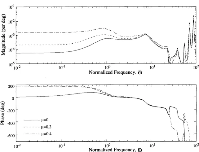
Figure 3-4 shows the frequency response G,o0(jC) in edgewise flight at various forward flight velocities. It is desired to actuate the servoflap in aileron reversal in order to provide sizable thrust control. Aileron reversal is the condition where positive servoflap deflection twists the blade enough to create a negative rotor thrust change. This is why the thrust output and servoflap input have 180 deg of phase difference, as observed in Figure 3-4, except at DC in the hover case (p = 0). The dynamic pressure at the servoflap location in hover case is not enough to provide sufficient moment for servoflap deflection to overcome the stiffness of the blade. Using softer blades would achieve aileron reversal easier. However, other problems arise such as instability caused by blade flutter. Aileron reversal of a blade is dependent on the torsional