An approximate dynamic programming approach to risk sensitive control of execution costs

An Approximate Dynamic Programming Approach to

MASSACHUSETS INSTTU't

Risk Sensitive Control of Execution Costs

OFSTECHNOLOGY

by

NOV

1 3 200

David Jeria

LIBRARIES

B.Sc., Massachusetts Institute of Technology (2006)

Submitted to the Department of Electrical Engineering and Computer

Science

in partial fulfillment of the requirements for the degree of

Master of Engineering in Electrical Engineering

at the

MASSACHUSETTS INSTITUTE OF TECHNOLOGY

June 2008

@

Massachusetts Institute

of Technology

2008. All rights reserved.

Author..

..

.

... ...

epartment of Electrical Engineering and Computer

Science

March 7,

2008

Certified by

.

.,

..---

.

...

Daniela Pucci de

Farias

Associate Professor

Thesis Supervisor

Accepted by

...

.

...

...

Arthur C. Smith

Chairman, Departmental Committee on Graduate Theses

An Approximate Dynamic Programming Approach to Risk Sensitive

Control of Execution Costs

by

David Jeria

Submitted to the Department of Electrical Engineering and Computer Science on March 7, 2008, in partial fulfillment of the

requirements for the degree of

Master of Engineering in Electrical Engineering

Abstract

We study the problem of optimal execution within a dynamic programming framework. Given an exponential objective function, system variables which are normally distributed, and linear market dynamics, we derive a closed form solution for optimal trading trajec-tories. We show that a trader lacking private information has trajectories which are static in nature, whilst a trader with private information requires real time observations to exe-cute optimally. We further show that Bellman's equations become increasingly complex to solve if either the market dynamics are nonlinear, or if additional constraints are added to the problem. As such, we propose an approximate dynamic program using linear program-ming which achieves near-optimality. The algorithm approximates the exponential objec-tive function within a class of linear architectures, and takes advantage of a probabilistic constraint sampling scheme in order to terminate. The performance of the algorithm re-lies on the quality of the approximation, and as such we propose a set of heuristics for its efficient implementation.

Thesis Supervisor: Daniela Pucci de Farias Title: Associate Professor

Contents

1 Introduction

2 The Trader's Problem

2.1 Market Impact and Price Dynamics . . . . . 2.2 An Exponential Utility Function ...

2.3 A Dynamic Program . ... 2.4 The Unconstrained Trader's Problem ...

2.4.1 Linear Dynamics without Information 2.4.2 Linear Dynamics with Information .. 2.5 The Curse of Dimensionality ...

2.5.1 Nonlinear Dynamics . ...

2.5.2 Adding Shortsale Constraints . . . .

13 .... ... . 15 ... 16 ... 18 ... ... 19 . . . . . . . . . 19 . . . . . . . . . 22 . ... 25 . ... 25 ... ... 27

3 On Linear Programming Approximations

3.1 Dynamic Programming via Linear Programming 3.2 Approximating the Value Function ... 3.3 Constraint Sampling ...

3.4 A Numerical Simulation with Linear Dynamics . 3.4.1 Choosing Basis Functions ...

3.4.2 Choosing a Sampling Distribution . .

A Proofs 41

List of Figures

2-1 Optimal trading strategies in the absence of information. T = 13, pi =

20, S = 105, 71,t = 10-5, 72,t = 10-7, t = 1000 and ,,=0.02 ... 21 2-2 Optimal trading strategies in the presence of information. T = 13,pl =

20, S = 105,yli,t - 10 5, 'Y,t 10-7, = 1000 and , = 0.02 . . . . . 24

2-3 The Need for Shortsale Constraints: Optimal trading strategies in the ab-sence of information. T = 13, pi = 20, S = 105, y, ₁ = 1.5 -10-5, l,t

10- 5 if t = 2, 3,...13, z2,1 = 10- 5, 72,t = 10- 7 if t = 2, 3,...13, a,,

1000 and ,= 0.02 ... ... .. 26 2-4 The Complexity Behind Short-Sale Constraints. A graphical representation

Chapter 1

Introduction

The problem of balancing risk and reward is one that is inherent to the stock market, and one that investors must understand well if they wish to outperform their peers. The basic premise behind portfolio theory states that, at every point in time, the portfolio manager must allocate a limited set of resources across stocks with diferring risk and return profiles, always with the goal of maximizing returns and minimizing risk. Markowitz, in 1952, formalized this thought process mathematically and introduced the notion of an efficient frontier: a curve over which a portfolio maximizes return given a certain level of risk. This concept is perhaps the most fundamental cornerstone of Modem Portfolio Theory. The original framework, however, overlooks a significant player in market dynamics, and one that has triggered much academic interest in the last decade: transaction costs. Transaction costs refer to the various costs of implementing a portfolio, and which derive mainly from the demand of liquidity. The majority of these costs can be traced back to comissions, bid/ask spreads, opportunity costs and price impact.

In 1988, Andre Perold studied the effects of these transaction costs on portfolio se-lection. He noticed that a hypothetical or "paper" portfolio consistently outperforms its actual portfolio. In one such example, he realizes that a hypothetical portfolio constructed according to the Value line rankings outperforms the Value Line Fund (the actual portfo-lio) by over 15%. Perold calls the difference in performance between the "paper" and the real portfolio its "implementation shortfall". The implementation costs, as he notes, can significantly offset returns if they are not managed appropiately, suggesting that a

portfo-lio manager not only wants to maximize return and minimize risk, he also wishes for his portfolio's shortfall to be minimized - that is, he wishes for the trades that will take him from a "paper" to a real portfolio to be optimally executed. Optimal execution, however, is a game of balance - if you execute too fast, your impact on liquidity will be large and your impact costs will increase, if you execute too slow, the inherent randomness of the mar-kets can cause unfavorable price movements. Almgren and Chriss (2000), using the same framework that Markowitz had devised 50 years before, elegantly model the intricacies of the inherent tradeoff between impact cost and timing risk that a trader faces when trying to achieve optimal execution. They introduce as well the notion of an efficient trading fron-tier, that is, the set of all trading trajectories that minimize cost for a given level of risk. Even though the analytical framework derived by Almgren and Chriss is still widely used, its underlying assumptions are no longer valid.

Almgren and Chriss develop their framework within a market that behaves linearly, that is, one in which impact costs are linear in the size of the executed order. This oversimplifies the highly complex market dynamics, thus producing trajectories which are suboptimal. Recent academic work strongly favors market dynamics which are nonlinear in nature, more specifically they favor a square-root model. Additionally, the Almgren and Chriss framework does not scale easily when there exist trading constraints. These constraints constitute any additional restrictions the trader might have when executing: a trader track-ing short-term capital gains might be restricted to executtrack-ing only within a certain price range, or a trader executing on behalf of a mutual fund might be restricted from short selling. In either case, the exclusion of these constraints from the optimization process significantly alters the shape of the resulting trading trajectories. The last point to be made regarding the Almgren and Chriss framework refers to the nature of their solutions: their chosen optimization method produces static trading trajectories. That is, it produces trad-ing curves that do not react to changes in market conditions. It is clear that an execution strategy which adapts dynamically to unforeseeable market conditions will, on average, outperform its static counterpart. As such, we wish to approach the problem of optimal ex-ecution within a framework that is both dynamic, and that is easily extendible to nonlinear and constrained systems.

In the following chapters, we provide an in-depth study of the problem of optimal exe-cution within a dynamic programming framework. This, however, is not a new approach: Bertsimas and Lo (1998) and Huberman and Stanzl (2005) both study optimal execution through dynamic programming. In Chapter 2, we replicate the results of Bertsimas and Lo (1998) and Huberman and Stanzl (2005) using an exponential objective function that allows for risk control. We show that, in a market with linear dynamics, a trader without private information does not benefit from the adaptive nature of the dynamic algorithm. On the other hand, however, we show that a trader with some prior information regarding the price dynamics, which we choose to model as an exponentially decaying stochastic pro-cess, only executes optimally when he does so in response to these real-time observations of the private information variable. We further show that once we add short sale constraints to the problem, or once we choose to model market dynamics with a nonlinear function, the algorithm ceases to give us a closed form solution for the optimal trajectories. Instead, the problem becomes exponentially hard to solve, and we are thus forced to approximating the optimal value function in the hope of finding a suboptimal solution that fits our needs.

In Chapter 3 we introduce the notion of Approximate Dynamic Programming via Lin-ear Programming. We show that the dynamic programming equations from Chapter 2 can be solvable via a nonlinear program. We further show that the exponential objective function is suitable for linearization, and we can thus solve an approximate version of our original problem using linear programming algorithms. The main advantage of the linear programming algorithm is that it the underlying model can easily incorporate nonlinear impact functions and shortsale constraints. However, the performance of the algorithm is highly dependent on a number of user input parameters. As such, we introduce each of these parameters and propose heuristics for each of them that are based on the results from Chapter 2.

Chapter 2

The Trader's Problem

Suppose a trader wishes to purchase S units of a security over a fixed time horizon [0, T]. For every unit length interval k E [0, T], the trader must determine the optimal number of units that he wishes to buy, st. When making such a decision, the trader seeks to find a balance between his immediate and his future costs, whilst maintaining his exposure to risk within a desired level. Risk, in our framework, refers to the uncertainty associated with the forecasted execution cost of any trading strategy. It mainly derives from the volatility of price and market volume. Costs, on the other hand, are associated with the market im-balances produced by trading. When liquidity is finite, there is an impact on the price of the security that comes from the associated increase in demand due to st. This impact on price has both a short-lived and a long-lived effect, and as expected, moves in a direction opposite to that which benefits the execution. These effects, commonly referred to as mar-ket impact, can be thought of as the difference between a price trajectory in which an order for st units was placed, and one in which it was not. Since both of these scenarios can-not be reproduced simultaneously, market impact has come to be known as the Heisenberg Uncertainty Principle of finance (Kissell and Glantz (2003)).

Bertsimas and Lo (1998) show that a trader seeking to minimize market impact will choose to trade evenly throughout the entire horizon. Nonetheless, this strategy ignores the underlying volatility of price and the opportunity cost that might arise from unfavorable price movements throughout the trading horizon. As such, we will assume that the objective function of the trader not only accounts for the expected cost of purchasing S units over the

trading horizon, but also accounts for the variance of such an execution strategy. If we let

st be the number of shares executed at price Pt, and we let V* be some variance associated

with the trader's degree of risk aversion, then the trader's problem can be summarized as:

mm E [t st s.t. var

ftstl

< V* t = f(Pt-lSt, t,Et) (2.1) Xt = V(Xt-I, V't) T E1st = S t=1 St > 0

where xt is a variable that predicts price, Et and vt are gaussian noise, and f(.) and g(.) are functions that model the dynamics of pt and xt respectively. Such dynamics will be further explored in the next section.

The problem formulated above can be approached using both dynamic and static opti-mization techniques. A static solution to Eq. (2.1) results in strategies that are determined a-priori, that is, st can be fully characterized using only information available at time t = 0. On the other hand, dynamic solutions will use information available up to time t - 1 to de-termine st. The nonnegativity constraint in Eq. (2.1), st > 0, is commonly referred to as a shortsale constraint. Bertsimas and Lo (1998) show that a dynamic solution to the risk-neutral (i.e., V* - oc) trader's problem with such a constraint is exponential in time. As such, they propose a static nonlinear optimization problem that, even though does not have a closed form solution, is indeed computationally feasible. Almgren and Chriss (1999) study the trader's problem in the case where shortsale constraints are ignored. Using a static optimization approach, they derive optimal trajectories, and introduce the concept of the Efficient Trading Frontier (ETF). The ETF is the curve in the mean-variance space that results from solving Eq. (2.1) across different values of V*:

(V*) = minE [ tstj :var

[

ptst < V* (2.2)

st t=1 _t=1

More recently, Huberman and Stanzl (2005) solve a dynamic version of Eq. (2.1) us-ing an additive-separable version of Bellman's equation with both expectation and variance terms. Assuming a linear price impact function with constant and positive slope, and ig-noring shortsale constraints, the authors arrive at a closed form solution for the traders problem. Using the same technique, they propose a recursive solution for the problem in which the price impact slope is time-dependent. Such a scenario derives from empirical evidence: Chan, Chun and Johnson (1995) find that the spread of NYSE stocks follows a U-shape pattern, thus suggesting that the slope of the price impact function should behave

similarly.

2.1

Market Impact and Price Dynamics

As was suggested previously, the market impact associated with the order of st units has both a temporary and a permanent component. The temporary market impact represents the cost from demanding liquidity, and possibly exhausting liquidity at various price levels. Such imbalances lead to price movements away from the equilibrium. However, once liq-uidity is reset, the price goes back to its equilibrium value. The permanent market impact, on the other hand, represents changes in the equilibrium price of the security, and as such, affects the cost of all subsequent trades.

We will define the temporary and permanent impact to be functions of the trade imbal-ance. From the trader's perspective, the trade imbalance at time t is given by st + Tt, where

rqt represents the residual trades in the market. We will further assume that {T

}[t=

are i.i.d. random variables, with zero mean and finite variances cr ,. Additionally, we assume knowledge of some variable xt that influences price. Such a variable can represent, for ex-ample, an expectation of liquidity for the particular asset of interest, or the expected return on an index that the asset might follow closely. Suppose that at time t, the equilibrium price

of the security is pt. The execution price, pt, is then given by:

pt = Pt + Tt (st + rt) (2.3)

Here, Tt (st + it) is the temporary impact function. Note that our model, as recent empirical studies suggest (Chordia et al. (2001)), allows for the temporary impact function to vary with time. Similarly, the equilibrium price at time t + 1 will be given by the discrete arithmetic random walk:

Pt+l = Pt + Pt (St + t) + It (xt) + Et (2.4)

The Et are random variables with zero mean and finite variance, o ,t, which represent

the volatility of the security at time t, Pt (st + rt) is the permanent impact function, and

It (xt) is a function that predicts price based on the information variable xt.

2.2

An Exponential Utility Function

The traders problem, as stated in Eq. (2.1), is to minimize execution costs while maintain-ing exposure to risk within a certain desired level. We can rewrite Eq. (2.1) as:

min E

piStv

f(*))

s.t. pt = Pt + Tt (st + rt) pt+I = pt + Pt (st + t) + I (xt) +t Et(2.5) (2.5) xt = g(xt it) T ZSt = S t=1 st > 0

where u (0, A) represents a utility function that captures the desired trade-off between cost and risk preference. Let u (0, A) = exp (AO), where 0 is a random variable representing the cost distribution of the execution strategy, and A represents the risk aversion coefficient of

the trader. If 0 is normally distributed, we have that:

E [u (0, A)] = E [exp (AO)]

= exp AE [0] + r)

We can readily see that with an exponential utility function, (2.5) is equivalent to a mean-variance optimization:

minE [exp (AO)] min {xp (AE [0] + 2(X)

}

= min E [0]+ 0

Alternatively, we can think of this problem in terms of the certainty equivalent cost. The certainty equivalent cost is defined as the fixed cost, 0c, whose utility is equal to the expected utility of the cost distribution, 0. An equivalent problem to (2.5) would be one in which we seek to minimize the certainty equivalent cost. If the cost distribution is normally distributed, we can solve for 0c:

exp (AO0) = E [exp (AO)]

= exp AhE [0] + -A01

And we conclude that 0, = E [0] + -2. We can again see the equivalence between (2.5) and a mean-variance optimization:

min E [exp (AO)] - min 0,

= min E [0] + }

The above equivalence, along with the multiplicative properties of the exponential func-tion, will make such a utility function of particular interest when formulating the trader's problem in a dynamic framework.

2.3

A Dynamic Program

Suppose that in the price dynamics equation (2.4), Et is normally distributed, such that

Pt also follows this distribution. We can now take advantage of the exponential utility

function, as was shown in the previous section, and we can restate the trader's problem as:

min E exp A ptst St t=1 s.t. t= + T (st + t) Pt+1 = Pt + Pt (st + Ut) + I (Xt) + Et T E St = S t=l st > 0

At any time t, the state of the above system can be fully described by the equilibrium price at time t, pt, the information variable xt, and the number of units that remain to be

sold, Wt = Wt-1 - st-1. These variables represent the information that is available to the

trader before he decides the number of units he plans to purchase at time t, st. Additionally,

we have the boundary conditions W1 = S and WT+1 = 0.

The dynamic programming algorithm relies on the fact that a sequence of trades that is optimal in the interval [0, T] will necessarily be optimal in the interval [t, T], for all t > 0.

If we let Vt (Pt, xt, Wt) be the optimal cost-to-go function when our state is (Pt, Xt, Wt), we

can translate the above condition into the following recursion:

Vt (ptt, Wt) = min E [exp (Aptst) Vt+l (pt+l, xt+, Wt+l)] (2.6)

st>O

Additionally, because of the boundary condition we require that

VT (PT, ZT, WT) = E [exp (APTWT)] (2.7)

Thus, the expected utility for the optimal trajectory st, ..., s will be given by:

V (pl,Xl, WO) min E exp A ktst plXlW1 (2.8)

si,...ST>O 0 E t

t=1

2.4

The Unconstrained Trader's Problem

As an initial approach to the constrained trader's problem, and in order to gain some insight about how solutions to it might behave, we will first consider the unconstrained version of the DP recursion presented in the previous section:

Vt (pt, t, Wt) = minE [exp (Aptst) Vt+1 (pt+, t+l, Wt+1)] (2.9) St

Since we require Pt to be normally distributed, the above equation can be simplified to:

Vt (Pt, Xt, W) = min exp (AE [p] st + s2var (Pt) E [Vt+1 (Pt+l, Xt+1, Wt+i)l

(2.10) Similarly, the boundary condition in Eq. (2.7) can be rewritten as:

VT (pT, X, WT) = exp AE [fT] WT + W2var (PiT) (2.11)

To solve the above system of equations, it will be necessary to fully characterize both the market impact functions as well as the dynamics of the information variable and the function lt (xt). In what follows, we solve the Trader's Problem when the dynamics of the system are linear, both with and without access to the information variable xt. The solu-tions will thus give us an understanding of the value of both information and its dynamic incorporation during execution.

2.4.1

Linear Dynamics without Information

We will quote a result by Huberman and Stanzl (2000), which states that when price impact is time stationary, only linear impact functions rule out arbitrage. This, in our framework,

refers solely to permanent impact, as temporary impact functions do not introduce arbi-trage. However, for simplicity, suppose that both the temporary and permanent impact functions are linear, and their slopes are time-dependent. In the absence of information, the price dynamics then become:

Pt = Pt + 71,t (St + 7]t) (2.12)

Pt+1 = Pt + '72,t (St + 't) + Et (2.13)

Under the above dynamics, the unconstrained trader's problem has a unique closed-form solution. The following theorem characterizes such a result.

Theorem 1. Suppose the price dynamics of the system follow Eqns. (2.12 - 2.13). Then, the recursion given by Eq. (2.10), with Eq. (2.11) as the boundary condition, has a unique solution given by.

ST-k O= kWT-k (2.14) VT-k (PT-k, WT-k) = exp (A -f (pT-k, WT-k)) (2.15)

f

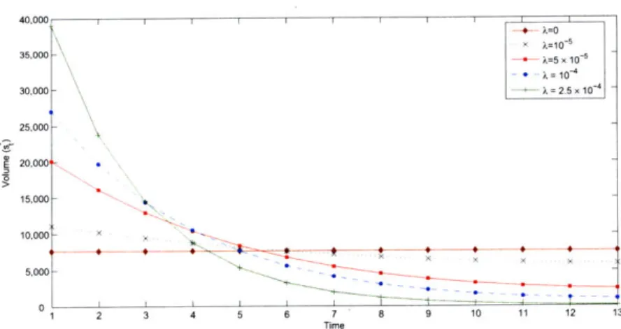
(pT-k, WT-k) = PT-kWT-k + akWT-k (2.16) for k = 0, 1,..., T - 1, where. (2ak-1 - 72,k) + A ( + 2,2k) (2.17) Ok = 2,k n k E k) (2.17) 2 (ak-1 + 71,k - 72,k) + / (,k r,k 2,k,k + ,k) ak = (1 ) k-1 + 2 (- 72,k%, + +k ,k) +k k - 2,k + , + 0kY2,k (2.18) with 0o = 1.

Somewhat against intuition, we realize that the optimal execution trajectory in the ab-sence of information is only a function of the size of the unexecuted order, Wt, and is

40,000 I I I k =10-5 35,000 ) =5 x 10 -5 , = 10-4 30,000- k= 25 x 10 25,000 -S20,000 15,000 10,000- x 5,000 S4 5 6 10 11 12 13 Time

Figure 2-1: Optimal trading strategies in the absence of information. T = 13, pi = 20, S = 105, 1,t = 10-5, 72,t = 10-7, =1000 and 2 , = 0.02

independent of the prevailing equilibrium price, pt. That is, the optimal strategy does not take advantage of intraday price observations. Instead, all the information needed to derive the sequence of optimal trades is known a-priori. Such a strategy is commonly referred to as being static, and provides a useful benchmark when assesing the real value of dynamic execution algorithms.

The question still remains, however: why is the optimal execution trajectory indepen-dent of price? The answer lies in the structure of the price dynamics. As can be seen, an observation of the equilibrium price at time t in no way helps us predict future values of the equilibrium price - the only variable which does so is our control variable, st. That is to say:

E [Pt+k - Pt+k-j Pt] = E [Pt+k - Pt+k-jl = 72,t+k-iSt+k-i

i=1

In other words, Pt gives no additional information as to whether it is preferable to execute at time t + k - j, or wait an additional j periods and execute at time t + k.

Figure 2-1 shows sample execution trajectories for different values of the risk-aversion parameter A. We readily recognize, for example, that a risk-neutral trader (A = 0) divides the order evenly throughout the trading horizon, as Bertsimas and Lo (1998) had previously

shown. Similarly, we also recognize that the optimal execution trajectory of a risk-averse trader (A > 0) will be decreasing in time, as shown in both Almgren and Chriss (2001) and Huberman and Stanzl (2005).

2.4.2

Linear Dynamics with Information

We will now explore the effect of information on the optimal execution strategy. Following Bertsimas and Lo (1998), suppose that the information variable follows a stationary AR(1) process:

xt = azt-1 + 6t (2.19)

where ca > 0 and 6t is a zero-mean gaussian variable with variance o 2t

Additonally, suppose that the function It (xt) is linear with a time-dependent slope. The price dynamics are then given by:

pt = Pt + 71,t (st + t) (2.20)

Pt+1 = Pt + 72,t (St + nt) + P2,txt + Et (2.21)

As in the previous section, given the above dynamics, the unconstrained trader's prob-lem has a unique closed-form solution. The following theorem characterizes such a result.

Theorem 2. Suppose the price dynamics of the system follow Eqns. (2.20 -2.21), and the information variable follows Eqn. (2.19). Then, the recursion given by Eq. (2.10), with Eq. (2.11) as the boundary condition, has a unique solution given by:

~_k = kXT-k + OkWT-k (2.22)

VT-k (PT-k,XT-k, WT-k)= exp (A -f (pT-k, T-k, WT-k)) (2.23)

f

(PT-k, XT-k, W = PT-k) T-kWT-k+ akT-k+ bkT-kT-k + C _k + dk

for k = O, 1,..., T - 1, where: ak abk-1 + P2,k Zk 2 2, 2 [p222 2 k (2ak-1 - 2,k) -A 2,krk +E,k [2,k + b_] 0.,k) Zk Zk = 2 (ak-1 + l71,k - '72,k) + A (0,k [k ,k ,2 2, k k + bk

~

]

2,k) ak = (1 - k) ak-1 + 2 (,,k o,k + 2,k + bl 1]

(

S71,k - 72,k + A k,k, + k2,k

bk = OkOk [2 (ak-1 + '1,k - ,) + A (,k [A7 + ,k +72k] + ,k + [,k + bk

]

,k] +

/k ['2,k - 2ak-1 - A ('2,k0,k + 0.,k+ k + [P 2,k + b ] 6,k2 +

Ok [-P2,k - abk-1] + P2,k + abk-1

Ck = k[_1 - 72,k + k7, [ + 72,k] 2,k + [Pi,k + b

]

O6,k +

2 277

1Ek

Ok [-P2,k - abk-1] + aCk-1

+

2Aa2 ,kC

l-dk = dk-1 ,kCk-1

(2.25) with bo = co = do = 0, Oo = 0 and Oo = 1.

The first difference to be noted between Eq. 2.14 and Eq. 2.22 is that the latter incor-porates observations of the information variable when determining the optimal execution trajectory. As such, the resulting strategy will be truly dynamic, since at time t, the opti-mal allocation of shares to be traded, st, depends on the observed value of the information variable, zt. This dependence, however, produces a somewhat counter-intuitive result, as is noted in Bertsimas and Lo (1998).

Bertsimas and Lo show that, given a risk-neutral trader with knowledge of a positively correlated information variable (i.e., A = 0, a > 0 and p > 0), the coefficient multiplying the information variable in Eq. 2.22 is positive -that is, Ok > 0. In our model, numerical

,e500

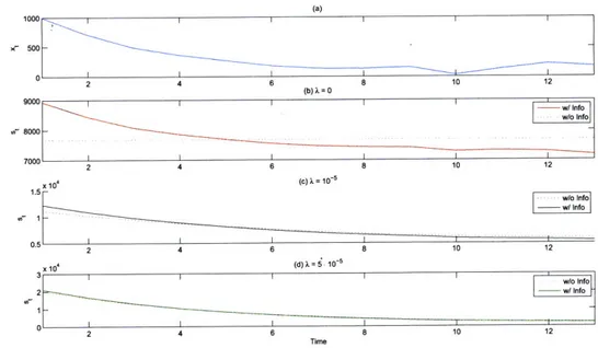
-2 4 6 8 10 12 (b)X=O w/ Info w/o Info .r8000 7000 24 6 8 10 12 x 104 (C) =10-5 1.5 w/o Info 0.₅ 2 4 6 8 10 12 x 10 (d) = - 10 - 5 w/o Info 2 W/ Info 1 1 2 4 6 8 10 12

Figure 2-2: Optimal trading strategies in the presence of information. T = 13, p =

20, S = 105, yl,t 10-5, 2,t = 10-7, 2 = 1000 and 2, = 0.02

traders as well. The apparent contradiction, then, is that positive observations of xt increase both the number of shares to be traded at time t and the equilibrium price to be seen at time t + 1. This result is particularly counter-intuitive when 0 < a < 1, since in this case we expect xt to decay exponentially to zero, and consequently, its contribution to the equilibrium price to decay to zero as well. This common misperception is solved by noting that the contribution of xt to the equilibrium price Pt is permanent. That is, a unit observation of xt not only implies an expected increase of p2,t on Pt+l, but also an expected

increase of P2,t + aP2,t+1 on Pt+2, and so on. From this we note that:

E [pt+k - Pt+k-jlPt,Xt] = (%,t+k-iSt+k-i + ak-ip2,t+k-it) i= 1

In other words, given an observation of xt, it is less costly to execute at time t + k -j, than

it is to wait

j

periods and execute at time t + k. The opposite is true when our observation

of xt is negative.

"front-load" with respect to their static benchmarks. This phenomenon is best seen in figure 2-2, which shows a sample trajectory of xt and the resulting optimal trajectories for different values of risk-aversion.

2.5

The Curse of Dimensionality

2.5.1

Nonlinear Dynamics

So far, the assumption of linear dynamics has proved to be a convenient framework for our problem: we have been able to derive closed form solutions for the Trader's Problem both in the absence and presence of information. However, markets do not behave linearly, and modelling both price and information dynamics as such is usually a poor design deci-sion. Incorporating nonlinear dynamics into our system will usually deter us from finding closed-form solutions. Nonetheless, certain dynamics might allow for numerical solutions to be available. The process behind finding such solutions is the same as that which we pre-sented earlier, in other words, the solutions is constructed using a set of recursive equations. Suppose the dynamics of our system are given by:

Pt = f(p (PSt-1, t- t-1, xt-1, Et-1) (2.26)

pt = g(t, st, rt) (2.27)

xt = h(xt-l, 6t-1) (2.28)

The boundary condition at time T is maintained, and given by:

VT (pT,XT, WT)= E [exp (A.(pT, WT, rl)WT)] (2.29)

Similarly, at time t < T, the recursion is given by:

Vt (pt, xt, Wt) = min E [exp (Ag(pt, Wt, 'rt)st) Vt+l (f(pt, st, t), xt, Et), h(Wx, 6t), t - st)]

St

x10, 4 r--4 -6 - - X -0 X=5 = 10-5 - - A= 2.5 10 8I I ! 2 4 6 8 10 12 Time

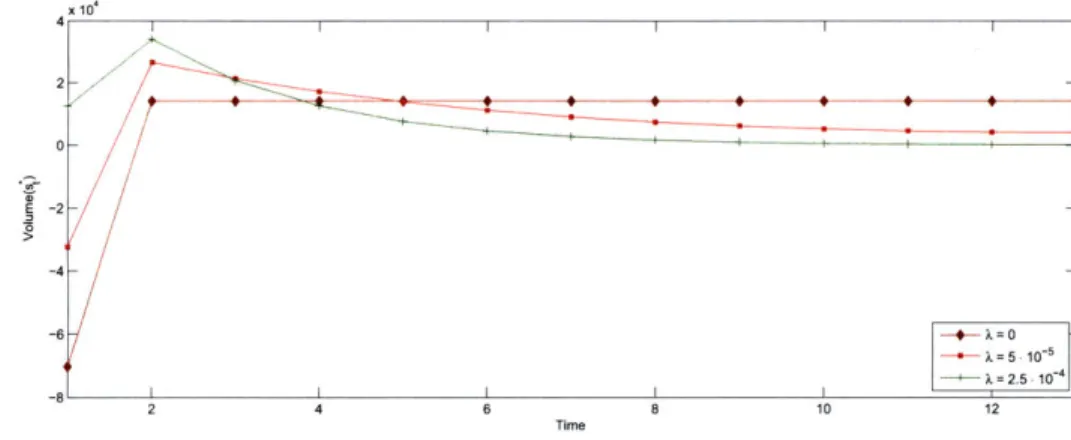
Figure 2-3: The Need for Shortsale Constraints: Optimal trading strategies in the ab-sence of information. T = 13,pl = 20, S = 105,71,1 = 1.5 - 10-5,,t = 10-5 if

t 2, 3, ... 13, 2,1 = 10- 5, 2,t 10- 7 if t = 2, 3,...13, 2, 1000 and2 =0.02

The optimal number of shares to be executed, s*, is then given as a function of the state variables:

st = arg min E [exp (Ag(pt, Wt, i7t)st) Vt+l (f (Pt, st, 77t, xt, Et), h(xt, 6t), Wt - st)]

St

= zt (ptXt, Wt)

(2.31)

Once V (-) has been found, initial conditions allow us to obtain s*. In the next time period, observations of the state variables allow us to obtain s*, and so on until we reach the end of the trading horizon. This process, in practice, is computationally expensive and often times intractable. As was suggested previously, closed form expressions for Vt (.) and s; (.) are usually not available. Instead, common practice is to store these functions using lookup tables: that is, for each possible combination of the state variables, we store the value which this functions maps to. It is easy to see that this practice becomes intractable quite easily, since the amount of space needed to store these lookup tables increases exponentially with the cardinality of our state-space and with the magnitude of our trading horizon.

-ST 1 0 < WT-1 S <<WT--0<s T-1 <WT1 S I I L I L o W_{T-1 ST-1

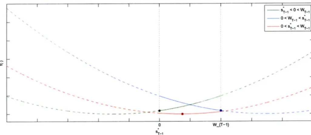
Figure 2-4: The Complexity Behind Short-Sale Constraints. A graphical representation behind Eqn. 2.32

2.5.2

Adding Shortsale Constraints

The non-negativity constraint of Eqn. 2.6 is commonly known as a short-sale constraint. It arises from the prohibition that certain financial institutions, such as mutual funds, have from short-selling. As such, optimally accounting for such a constraint becomes of impor-tance. The solution to the unconstrained problem from equation 2.14 suggests that such constraints are not binding unless Ok < 0. This, in turn, translates to conditions in the dy-namics of both the price-impact slopes and variance terms. For example, Figure 2-3 shows the optimal trajectories associated with a system in which the price-impact slopes of the first period is larger than that of the remainding periods. The trajectories suggest that a trader with a low risk-aversion will want to short a number of stocks in the first period, a result which certain institutional investors might be prohibited from implementing. Im-posing such a constraint in a dynamic optimization framework, however, adds a level of complexity to the problem which renders it unfeasible.

The added complexity from short-sale constraints is a result of the recursive nature of dynamic programming. Suppose, as was done in Section 2.4.1, that the price-impact functions are linear. Equation 2.15 of Theorem 1 states that the optimal cost-to-go function of the unconstrained problem, V(.), is of the form exp(f(.)), where f(.) is quadratic in the state variables of the system. We will refer to this functional form as an

exponential-quadratic composite function. Consider now what happens once non-negativity constraints are added.

At time T the optimal control is given by s = WT, and the optimal cost-to-go function,

VT(.), will be an exponential-quadratic composite function, as can be easily verified. As

such, in the T - 1st period we will want to minimize an exponential-quadratic composite function subject to a non-negativity constraint of the form 0 < s*_ < WT-1. Since the exponential function is monotonic, we are only concerned with the minimization of the quadratic function. Given the nature of the constraint, however, the value of the constrained optimal control, sT-1, will be a piecewise function of the value of the unconstrained optimal control, sT_ :

0 if s*-1 < 0 < WT- ₁

T-1= if 0 < ST_ < WT-1 (2.32)

WT-1 if 0<WT-1 < S*1

The piecewise nature of the solution, in turn, causes VT-1 (.) to be piecewise as well. As such, VT- I(-) will be represented by a different exponential-quadratic composite function

in each of these intervals. In the T - 2nd period, a similar process will occur, and each of the three intervals over which VT- 1 (-) is defined, will have to be subdivided into another

three intervals. Thus, both ST-k and VT-k(') will be piecewise functions defined over

3k different intervals. The complexity of such a problem becomes problematic when the number of periods T becomes large, and as such, devising approximation methods that deal with the added complexity becomes of importance.

Bertsimas, Hummel and Lo (1999), recognizing the complexity of a constrained-optimization problem in a dynamic setting, propose a static approximation method as a mean of extract-ing a near-optimal execution strategy. Such a technique, however, sacrifices the value of intraday information...

Chapter 3

On Linear Programming

Approximations

As was seen in the previous section, the recursive nature of dynamic programming ren-ders it an unfeasible technique for systems with either a large state space or an extensive time horizon. Such is the case in the constrained Trader's Problem, and for this reason, ap-proximation algorithms become of importance. The classical papers in the field opt towards static optimization techniques as the chosen means for reducing complexity. This, however, comes at the cost of sacrificing real-time information, and the value that such observations might add to the resulting execution strategies. Because of this, we desire an approximation algorithm that reduces complexity whilst maintaining its dynamic adaptability. Many such algorithms exist -the field of approximate dynamic programming is one of great interest in the academic world -however, none have been applied to the problem being studied in this paper. One such technique, the one we will be concerned with, involves approximating the optimal value function within a class of linear architectures. Such linearization not only reduces complexity, but allows us to take advantage of well-known linear programming techniques for the generation of near-optimal solutions.

In what follows, we will introduce the theory behind linear programming approxima-tions, always within the framework of the Trader's Problem that was introduced in the previous chapter.

3.1

Dynamic Programming via Linear Programming

Recall the dynamic program that was introduced in §2.3:

Vt (pt, zt, Wt) = min E [exp (Aptst) Vt+l (Pt+l, xt+l, Wt+)

st>O

VT (pT, XT, WT) = E [exp (AT WT)]

We notice that, if Pt is normally distributed for all t, the above DP can be simplified to:

V (Pt,

zXt,

W) = min exp AE [ft] + S2vr (P) E [V+l (pt+,

xt+,,

W +1)

VT (PT, XT, WT) = exp AE [PTr] WT + 2W 2var (PT)

For simplicity, let i- = (Pt, Xt, Wt), and suppose that the system dynamics are given by:

rt+l = f(M, t, ,Ect)

Define the cost function c(r, st, rTt) as:

C(Vt St, t) = exp (AE [g(t, st, rt)] st + 2tvar (g(Ft, st, it)) (3.1)

Also, define the operator T such that:

TVt+l(Tt+1) = min {c(rt, st,rjt) E [Vt _{(t+l ) Ftj]} (3.2)}

stESt

where St =

{st

: 0 < st < Wt }. The DP recursion can now be written as:

Vt(t) = TVt+ 1(f(T, st, Et))

(3.3)

VT (r) = c(,

WT, TI)

The next proposition presents a nonlinear program that solves the above set of recursive equations:

Proposition 1. Consider the problem:

maxv,(,)

V(T1) s.t. Vt(t) < TVt+l(t+,),

VT(:) = C(7T, WT, TIT),

Vt, t E Rt V(T E R T (3.4)

where 7 is the set of all possible values attained by the state variables, rt. If Vt* (-) is the unique solution to (3.3), then Vt* (.) is also the unique solution to (3.4).

Before the proof of this proposition, we present a lemma that leads to the result, and that introduces an important and well-known property of the DP operator:

Lemma 1. The operator T is monotonic, that is:

V < V = TV < TV

The monotonic property of T, in turn, leads to the result presented in the following corollary:

Corollary 1. A feasible solution Vt (.) to (3.4) is a lower bound to the optimal value func-tion, Vt* _).

Given that T is montonic, we are now ready to prove Proposition 1:

Proof Suppose Vt* (.) solves the optimality equations given in (3.3) such that Vt (.)

-TV,;*(.) for all t. Additionally, let t(-) be any feasible solution to (3.4). From the con-straint set, we have that:

VT-I,(.) TVT(.)

- TV (.)

VT- 1(.) < Vl (-), we proceed similarly for VT-2(.), and conclude that:

VT-2 () < TVT_1()

< TV_ (), by monotonicity = V- 2 (.), by optimality

Proceeding similarly, we conclude that V(') < V*(.) for all t (Corollary 1).

From Corollary 1 we know that V (.) < V*(). It follows that the unique feasible solution which maximizes this constraint is that which achieves equality, that is, VI(-) = V*(.). It remains to be shown that V = V*(.) for all 1 < t < T. Consider the followingV() inequalities:

< T V2(.), by feasibility

< TV2*(.), by monotonicity

We also know from the optimality condition that V1() = V* (.) = TV* (.). Thus, we have

that TV2* () < TV2(.) < TV2* (.), and conclude that V2(.) = V2*(.). Proceeding similarly

for t = 3, ...T, we conclude that V (-) = Vt*(.) for all t (Proposition 1). O

As was suggested previously, we want to take advantage of linear programming algo-rithms for the generation of near-optimal solutions. However, since T is nonlinear, the constraint set of (3.4) is nonlinear as well. We get around this by realizing that, given t, the constraint Vt (K-) < TVt+1(T+1) is equivalent to the set of constraints given by:

Vt (,t) < c(T, st, lt) - E [Vt+l(+1)], Vst (E St (3.5)

The above statement is important not only because it allows us to set up the DP recursion as an LP, but it also allows us to get rid of the minimization implicit in the T operator. As was mentioned previously, this operation can become computationally expensive with certain

nonlinear cost functions. We now formulate (3.3) as a linear program: maxvt,) V(Fi) s.t. Vt(r-) c (t, st, Tt) -E [Vt+l('t+l)] ,

V (C)

c(,T,

rl, ),

Vt, Kt E t, st E St VT E RT

With respect to the structure of the LP, we readily recognize that the complexity of the problem still renders it unfeasible: the LP presented in (3.6) has as many variables as it has states, and as many constraints as there are state-action pairs. In the upcoming section, we will present an approximation algorithm that drastically reduces the number of variables, and that deals efficiently with the constraint set.

3.2

Approximating the Value Function

Consider approximating the optimal cost-to-go function by a linear combination of basis

functions. That is, given a set of preselected basis functions k : t H R, k = 1,..., K,

we wish to generate weights Wt,k such that:

K

Vt(7) Vt) CWt,kk(ik=,E

kI

Vt, r E Rt (3.7)

Substituting the above approximation into (3.6) effectively reduces the problem into an optimization over the weighting parameters, wt,k, thus decreasing the number of variables to only T x K. The linear program that solves for these is given by:

K max,,k Wl,k k(1) k=l K K s.t. Wt,kJk( <t) C(', St, 't) E Wt+l,kE [k( T+1)t1 , k=l k=l K 0 WT~(bkT)

C=

(i,

WT, IT), k=1 Vt, t E R t,St E St (3.8)

(3.6)

From Corollary 1, we know that the solution to (3.8) is a lower bound to the optimal value function. More precisely, it is the tightest lowest bound among approximations of the form given in (3.7). This, however, does not mean much if the set of basis functions are a poor approximation to Vt(.). The implicit assumption behind the selection of the k (.) is

that they are selected such that a few of them can approximate the optimal value function accurately. In other words, the solution given to us by (3.8) will only be as good as the choice of basis functions we make. Unfortunately, the preferred method for selecting such basis functions is one based mostly on heuristics, as we will explore in the case study at the end of the chapter.

3.3

Constraint Sampling

The exact LP in (3.6) is unfeasible both for its number of variables as well as its constraints. As was seen in the previous section, the number of variables can be effectively reduced by approximating the value function within a class of linear architectures. However, finding an optimal solution to the approximate LP in (3.8) still requires an unmanageable number of constraints - more specifically, one constraint per state-action pair. We thus require a method to reduce the number of constraints whilst maintaining the accuracy of our approx-imation. De Farias and Van Roy (2004) show that, under certain assumptions, constraint sampling is an effective method to reduce the complexity of the ALP. More explicitly, they show that given a set Q with k state-action pairs sampled from a distribution 0, the solution to the reduced linear program (RLP) is probabilistically close to that of the ALP. That is, if i is the solution to the RLP and ? is the solution to the ALP, we have that:

Pr(IIV* - 4Il - IV* - I II <_ CV*D) > 1 - 6

where c and 6, representing error tolerance and level of confidence respectively, are in-versely related to the number of constraints k. Although the work by de Farias and Van Roy focuses on infinite-horizon Markov Decision Processes (MDP's), their framework is also applicable for the finite-horizon problem being studied.

3.4 A Numerical Simulation with Linear Dynamics

In what follows, we study the implementation of the algorithm in (3.8), more particularly we will look at it in terms of the system which was studied in §2.4.2. That is, we will study the execution of a risk-averse trader who posseses private information in a market with linear dynamics. As was mentioned previously, choosing linear dynamics to model price evolution and impact is usually a poor choice. However, the closed-form solutions that we found for the Unconstrained Trader's Problem gives us a good benchmark with which to compare the performance of the approximate linear program. Recall the dynamics of the system's variables: At = Pt + Yit (st + t) Pt+l = Pt + '2,t (St + rlt) f P2,tXt + Et Xt+1 = aOXt + t+1i Wt+1 = Wt - st

The cost function from (3.1) can be rewritten as:

c(pt, St) = exp (APtst + A Y7,t + 2 0 t

3.4.1

Choosing Basis Functions

As was mentioned previously, the process for selecting basis functions is mainly an em-pirical one. As such, we will use the results obtained in §2.4.2 as the foundation for our choice of basis functions. Recall, from Theorem 2, that the optimal value function for the Unconstrained Trader's Problem was given by:

VT-k (T-k) = exp (A .

f

('T -k))

A first choice of basis functions comes from the series expansion of the exponential func-tion when higher order terms are ignored, that is:

E [VT-k (T-k)] = E [exp (A.

f

((T-k))] (3.9)

= exp Af (Tk) + var ((T-k)) (3.10)

A2

1 + Af (T-k) + -var (f (T-k)) (3.11) Since var(ptWt)= (7,t-1 1 + 1 ,t-1) t2, and var(xtWt) = o, t-1T 2, it suffices with

a single basis function that accounts for Wt2 such that the variance of the value function gets effectively incorporated into the set of constraints. In other words, a possible set of basis functions to approximate the optimal value function would be:

01(-) = 1

P2 () = pt

Wt

03(') = W2 (3.12)

The above selection has its shortcomings, however. As was seen in Chapter 2, the in-clusion of nonnegativity constraints in the Trader's Problem resulted in VT-k(') being an exponential-quadratic piecewise function over 3k different intervals. We can deal with the

piecewise nature of VT-k() by defining a partition over the state space, and we can take advantage of the approximation in (3.11) to arrive at a set of basis functions that are both compact and accurate. We can thus approximate the value function with an improved set of basis functions given by:

1(q, iEIT 1 2(ri), r 2

where n, represents the set of states in partition n. Since partitioning the state space in-creases the number of variables of the linear program, it is necessary that the partition be as compact as possible. For this purpose, we can look back at our results from the non-constrained problem and use those to make an educated guess for an efficient partition. Recall from equation (2.22) that the optimal trade size in a system with linear dynamics with private information is a function of the information variable, xt, and the remaining trade size, Wt. This suggests that an effective state space partition would be one that incor-porates these two variables and excludes the price variable, Pt.

3.4.2

Choosing a Sampling Distribution

As was discussed previously, the number of constraints, one per state-action pair, is restrict-ing in the evaluation of the ALP. The constraint samplrestrict-ing scheme studied by de Farias and Van Roy (2004), and introduced in a previous section, is one of the means through which the cardinality of the constraint set can be reduced. To implement this scheme effectively, and to guarantee that the solution to the RLP is not far'from that of the ALP, it is necessary to choose a sampling distribution such that the subset of constraints that are not satisfied have a minor impact on the feasible region of the RLP.

Recall the dynamics of the system in hand: both the price variable, pt, and the informa-tion variable, xt, are normally distributed around mean values pl and xl respectively. Also, the remaining state variable Wt is a function of st-1. These particular dynamics suggest that an appropriate sampling scheme would be one that generates state-action pairs where

pt and xt are normally distributed, while Wt and the action variable st belong to integer sets. That is, we define sets Pt, Xt and

Nt

such that:

2 2 2

t = (Pt : Pt N(pt-1,72,t-1o,t--1 + P2,t-10'tt-1 +

t-Xt = {xt : N(xt-1

t

2t

Ht = (Wt : Wt ( [O, Wt-1 - St-1] C Z}

and we define the subset of sampled states as:

Qt = {(pt, xt, 1t) : Pt E Pt, t E Xt, Wt E Ht, andPtI = IXt

_{Nt| = k}}

where |A is the cardinality of set A, and k is the number of constraints in Qt. Finally, the RLP is then:

K maxk E Wl,kk(rl)

k=l

K K

s.t. E Wt,kOk (t) < C(t, St, It) E Wt+l,kE[Ok(t+l)l t ,

k=1 k=1 K E l, Tkk(T) = TT), k=1 Vt, Tit E t, St C St VI'T E QT (3.13)

Chapter 4

Conclusions

The last 20 years have seen dramatic changes in the stock market. The vast technological advances have prompted an era in which the computer is the center of the trading process. This, together with a number of other factors (the decimalization of the New York Stock Exchange, for example) have resulted in a drastic change of maker dynamics: liquidity has increased, spreads have narrowed, and competition among portfolio managers has signif-icantly reduced profit margins. As such, the need to maximize returns optimally at every point of the investment process has become key. In one such point, much effort has been placed on the optimal control of execution costs. The problem of executing optimally is stochastic and dynamic by nature, and as such, adapts quite well within the framework of dynamic programming. The complexities behind modelling market dynamics, however, many times render a recursive DP algorithm unfeasible. As such, there is indeed a need for an algorithm that will be able to have the adaptive nature of DP, while not oversimplifying the dynamics that control our system.

In this thesis we introduce the problem of optimal execution. We examine it within a dynamic programming framework: first, using simple linear dynamics, then adding an information variable, and lastly including shortsale constraints. As can be seen, the increase in complexity leads us to a point where a simple DP recursion is an unfeasible method for solving the problem in hand. As such, we introduce the notion of approximate dynamic programming via linear programming. The algorithm introduced allows for the inclusion of complex market dynamics and additional trading constraints, and even though its solution

might be suboptimal, there is value added due to the accurateness of the underlying model. The implementation of the algorithm is key to its performance. The linearization of the objective function, and the constraint sampling scheme are only two of the inputs that de-termine the quality of the algorithm's output. As such, the detailed analysis done in Chapter 2 gives us a good starting point for the selection of these varied inputs. However, further analysis is necessary in order to accurately evaluate the performance of the algorithm's so-lution. Increased complexity always comes at the cost of performance, and as such there exists the need to find a balance between these two.

Appendix A

Proofs

A.1

Theorem 1

Proof The proof will follow a simple induction argument. The base case, for k = 0, is

trivial, and is given by:

s* = WT

VT (PT, xY, WT) = exp (A [pTWT + P1,TXTWT + (7)1,T +

Assume now that Eqns.(2.14-2.15) are valid for T - k + 1. We will now show that they

are true for T - k. We then have that:

VT-k (PT-k, XT-k, WT-k) = min

ST-k

exp (AE [PT-k ST-k + 2 kvar T (+ ))

XE [VT-k+1 (PT-k+1 XT-k+l, WT-k+1)]

From the induction assumption we know that:

E [VT-k+1 (')] = exp (A [(E [PT-k+1 + aT-k+1E [XT-k+1]) WT-k+1J) X

exp (A

(

bT-k+ + [var (PT-k+)

+

a2k+1ar (XT -k+1)]) T_

Taking the first-order condition for VT-k (.) yields (2.14) to be the unique minimum. O A 2 2

2 'Y' T17 T

W]T

Bibliography

[1] Adelman, D. 2006 "Dynamic Bid-Prices in Revenue Management" Operations Re-search

[2] Almgren, R. 2001 "Optimal Execution with Nonlinear Impact Functions and Trading-Enhanced Risk"

[3] Almgren, R., and Chriss, N. 2000 "Optimal Execution of Portfolio Transactions"

Journal ofRisk 3 5-39

[4] Almgren, R., and Chriss, N. 1998 "Optimal Liquidation"

[5] Almgren, R., Thum, C., Hauptmann, E., and Li, H. 2005 "Direct Estimation of Equity

Market Impact"

[6] Bertsekas, D., 1995 Dynamic Programming and Optimal Control Vol. I and II. Bel-mont, MA: Athena Scientific

[7] Bertsekas, D., and Tsitsiklis, J. 1996 Neuro-Dynamic Programming Belmont, MA: Athena Scientific

[8] Bertsimas, D., Hummel, P., and Lo, A. 1999 "Optimal Control of Execution Costs for Portfolios"

[9] Bertsimas, D., and Lo, A. 1998 "Optimal Control of Execution Costs" Journal of

Financial Markets 1 1-50

[10] Bertsimas, D., Hummel, P., and Lo, A. 1999 "Optimal Control of Execution Costs for Portfolios"

[11] Bertsimas, D. and Tstitsiklis, J. 1997 Introduction to Linear Optimization Belmont, MA: Athena Scientific

[12] de Farias, D. P. 2002 "The Linear Programming Approach to Approximate Dynamic Programming: Theory and Application" Ph.D. Thesis Stanford University

[13] de Farias, D. P., and Van Roy, B. 2003 "The Linear Programming Approach to Ap-proximate Dynamic Programming" Operations Research 51 850-865

[14] de Farias, D. P., and Van Roy, B. 2004 "A Cost-Shaping Linear Program for Average-Cost Approximate Dynamic Programming with Performance Guarantees"

[15] de Farias, D. P., and Van Roy, B. 2004 "On Constraint Sampling for the Linear Pro-gramming Approach to Approximate Dynamic ProPro-gramming" Mathematics of

Oper-ations Research Vol. 29 No. 3 462-478

[16] Huberman, G., and Stanzl, W. 2005 "Optimal Liquidity Trading" Review of Finance 9 165-200

[17] Huberman, G. and Stanzl, W. 2004 "Price Manipulation and Quasi-Arbitrage"

Econo-metrica 72(4) 1247-1275

[18] Kisell, R., and Glantz, M. 2003 Optimal Trading Strategies: Quantitative Approaches

for Managing Market Impact and Trading Risk New York, NY: Amacom

[19] Obizhaeva, A. and Wang, J. 2004 "Optimal Trading Strategy and Supply/Demand Dynamics"

[20] Perold, A. 1998 "The Implementation Shortfall: Paper Versus Reality" Journal of