Dynamic event tree analysis method (DETAM) for accident sequence analysis

DYNAMIC EVENT TREE ANALYSIS METHOD (DETAM) FOR ACCIDENT SEQUENCE ANALYSIS

by

C. G. Acosta and N. 0. Siu Massachusetts Institute of Technology

Nuclear Engineering Department MITNE-295

October 1991

Final Report

Grant Number NRC-04-88-143

"Physical Dependencies in Accident Sequence Analysis"

Project Officer: Thomas G. Ryan Office of Nuclear Regulatory Research United States Nuclear Regulatory Commission

DYNAMIC EVENT TREE ANALYSIS METHOD (DETAM) FOR ACCIDENT SEQUENCE ANALYSIS

by

C. G. Acosta and N. 0. Siu Massachusetts Institute of Technology

Nuclear Engineering Department MITNE-295 October 1991 Final Grant Number "Physical Dependencies in Report NRC-04-88-143

Accident Sequence Analysis"

Project Officer: Thomas G. Ryan . Office of Nuclear Regulatory Research United States Nuclear Regulatory Commission

ABSTRACT

In recent years, there has been a growing sentiment that the conventional event tree/fault tree methodology, used in current nuclear power plant probabilistic risk assessment studies, has weaknesses in treating complex scenarios whose development is strongly affected by operator actions. This .report discusses these weaknesses, reviews potential alternative methodologies, and proposes an improved approach, called the Dynamic Event Tree Analysis Method (DETAM), designed to analyze the risk associated with dynamic nuclear power plant accident sequences.

DETAM provides a framework for treating stochastic variations in operating crew states (defined by substates characterizing the accident diagnosis, the planned actions, and the crew quality) as well as stochastic variations in hardware states. Plant process

variables, used when determining the likelihood of stochastic branchings, are treated

deterministically. Scenario truncation and grouping mechanisms are employed to limit the size of the model.

To demonstrate the capabilities of DETAM, it is applied towards the analysis of a steam generator tube rupture (SGTR) accident. This application shows that the

methodology can be practically employed in realistic analyses, and that useful insights concerning potential risk contributors (e.g., scenarios and dependencies not identified by conventional models) and the effectiveness of operating procedures can be generated.

TABLE OF CONTENTS Page ABSTRACT TABLE OF CONTENTS ii LIST OF TABLES iv LIST OF FIGURES v ACKNOWLEDGMENTS vi 1.0 INTRODUCTION 1 1.1 Background 1

1.2 Conventional Event Tree/Fault Tree Analysis 2

1.3 Dependencies in Accident Sequence Analysis 6

1.4 Summary 8

2.0 ALTERNATIVE METHODOLOGIES FOR DYNAMIC SCENARIO ANALYSIS 13

2.1 Introduction 13

2.2 Event Tree Limitations 15

2.3 Expanded Event Trees 16

2.4 Analytical Methodologies 18

2.4.1 Event Sequence Diagrams 18

2.4.2 GO-FLOW 20

2.4.3 Markov Models 21

2.5 Simulation Methodologies 25

2.5.1 DYLAM 25

2.5.2 Discrete Event Simulation 27

2.6 Evaluation of Methodologies 30

3.0 DYNAMIC EVENT TREE ANALYSIS METHOD (DETAM) 50

3.1 Introduction 50

3.2 General Concept 50

3.3 General Implementation for Accident Scenario Analysis 52

3.4 Discussion 53

4.0 DETAM APPLICATION - MODEL CHARACTERISTICS 59

4.1 Introduction 59

4.2 Steam Generator Tube Rupture Events: Description and Analysis 59

4.2.1 SGTR General Progress 59

4.2.2 Seabrook SGTR Model 61

4.2.3 Sequoyah SGTR Model 62

4.3 Thermal-Hydraulic Model for SGTR 63

4.3.1 Description 64

4.3.2 Model Validation 65

4.4 Hardware Model 66

4.5 Operator Crew Model 67

4.5.1 Basic Fo-mulation 67

4.5.2 Crew Diagnosis State 68

4.5.2.1 General Scenario Component 68

4.5.2.2 Safety Functions Component 69

4.5.3 Crew Quality State 69

TABLE OF CONTENTS (cont.)

Page 4.5.4 Crew Planning State

4.5.4.1 Procedure-Based Planning 4.5.4.2 Non-Procedural Actions 4.5.4.3 Planning State Transitions

4.5.6 Operator Error Forms That Can Be Modeled 4.6 Frequency Assignments

4.6.1 Hardware System Failure Rates 4.6.2 Diagnosis State Transition Rates 4.6.3 Planning State Transition Rates 4.6.4 Performance Error Rates

4.7 Branching Rules

4.8 Stopping Rules and Truncation Mechanisms 4.8.1 Absorbing States

4.8.2 Scenario Truncation on Low Likelihood 4.8.3 Similarity Grouping

4.9 DETAM Computer Code for SGTR (DETCO-SGTR) 4.10 Summary Remarks

5.0 DETAM APPLICATION - RESULTS 5.1 Introduction

5.2 DETCO-SGTR Runs Performed and Results Obtained 5.3 Practicality of DETAM

5.4 Capabilities of DETAM

5.4.1 Treating Event Ordering and Timing 5.4.2 Operator Error Forms

5.4.3 Consequences of Operator Actions 5.4.4 Context for Likelihood Assignment 5.4.5 Modeling Actual Incidents

5.5 Comparison of DETAM and Conventional PRA Results 5.5.1 End State Comparison

5.5.2 Partial Sequences 5.6 Other Results 5.6.1 SGTR Procedures 5.6.2 Impact of Instrumentation 5.6.3 Dependent Failures 5.7 Summary 6.0 CONCLUDING REMARKS 6.1 Introduction

6.2 Advantages and Disadvantages of DETAM Approach 6.3 SGTR Application Results

6.4 Potential Applications 6.5 Future Work

REFERENCES

APPENDIX A - Thermal-Hydraulic Model

APPENDIX B - Walk-Through of Dynamic Event Tree

70 70 71 71 71 72 73 73 74 75 75 76 76 77 77 77 78 104 104 104 106 107 107 108 108 109 109 110 110 111 114 114 115 115 116 128 128 128 129 130 130 133 to be supplied to be supplied iii

LIST OF TABLES

No. Title P age

2.1 Control Laws for Holdup Tank Problem [9] 33

2.2 Characteristic Parameters for Tank Problem [9] 33

2.3 GO-FLOW Signals for Holdup Tank Problem 34

2.4 GO-FLOW Time Points for Holdup Tank Problem 34

2.5 GO-FLOW Computation Chart for Holdup Tank Problem 35

2.6 DYMCAM Rules for an Active Component {47] 37

3.1 Dynamic Event Tree Characterization of DYLAM 56

3.2 Characteristics of Dynamic Event Trees for Accident Scenario 56 Analysis

4.1 Seabrook PRA SGTR Top Events [61 80

4.2 Sequoyah PRA SGTR Top Events [5] 80

4.3 Process Variables Carried in Dynamic Event Tree Model for SGTR 81

4.4 Systems Included in DETAM SGTR Analysis 82

4.5 Scenario Transition Parameters 83

4.6 Scenario Transition Criteria 83

4.7 Diagnosis State Parameters . 84

4.8 Response to Reactor Trip or Safety Injection Procedure Steps (E-0) 85 4.9 Loss of Secondary Heat Sink Procedure Steps (FR-H.1) 86 4.10 Loss of Reactor or Secondary Coolant Procedure Steps (E-1) 86 4.11 Steam Generator Tube Rupture Procedure Steps (E-3) 87 4.12 Nominal Transitions from Reactor Trip or Safety Injection 88

Procedure (E-0)

4.13 Nominal Transitions from Loss of Secondary Heat Sink Procedure 89 (FR-H.1)

4.14 Nominal Transitions from Loss of Reactor or Secondary Coolant 91 Procedure (E-1)

4.15 Nominal Transitions from Steam Generator Tube Rupture Procedure 92 (E-3)

4.16 Hardware Failure Frequencies 93

4.17 Qualitative Likelihoods 93

4.18 Likelihood of Incorrect Scenario Diagnosis During An SGTR Event 94

4.19 Meta-Rules for Prccedure Transitions 94

4.20 Transition Likelihood from Procedure E-0 to E-3 95

4.21 Likelihood that the Operator Crew Skips a Step While in E-0 95 Procedure

4.22 Likelihood that the Operator Crew Turns Off HPIS 96 4.23 Likelihood that the Operator Crew Starts Bleed and Feed Cooling 96

5.1 DETAM Runs Performed 117

5.2 Most Frequent End States (Runs 2-7) 118

5.3 Distribution of the Time to Initiate Cooldown and 119

Depressurization (Run 2)

5.4 North Anna 1 SGTR Chronology of Events [63] 120

5.5 Ginna SGTR Chronology of Events [60,61] 120

5.6 Comparison of Conventional and Dynamic Event Tree End State 121 Conditional Frequencies

5.7 Conditional Split Fractions [5,6] 122

LIST OF FIGURES

No. Title P age

1.1 Portion of Sequoyah Event Tree for SGTR [5] 9

1.2 Portion of Seabrook Frontline Systems Early Response Tree 10 for SGTR [6]

1.3 Simplified Event Tree Representation of TMI-2 Accident [11] 11

1.4 Event Tree for Seabrook Top Event SL [6] 12

2.1 Holdup Tank Problem [9] 38

2.2 Simple Hardware-Oriented Event Tree for Holdup Tank Problem 39

2.3 Event Sequence Diagram for Holdup Tank Problem 40

2.4 Expanded Event Tree for Davis Besse Event (6/9/85) [28] 41 2.5 Initial Portion of Expanded Event Tree for Holdup Tank Problem 42 2.6 Event Sequence Transition Representation of an SLOCA Accident [12] 43 2.7 Possible Sequences of Transitions for the SLOCA Event Tree [12] 43 2.8 GO-FLOW Chart for Holdup Tank Problem (First Two Phases) 44

2.9 GO-FLOW Operators [20,36] 45

2.10 Example Application of DYLAM to Holdup Tank Problem 46

2.11 Example Dynamic Evolution of Master Schedule 47

2.12 Tank Level History (One Discrete Event Simulation Trial) 48

2.13 Generic Component Model for DYMCAM 49

3.1 Example Dynamic Event Tree for Two Binary Systems 57

3.2 Tasks Performed During A Single DETAM Time Step 58

4.1 Portion of Seabrook Frontline Systems Early Response Tree 97 for SGTR [6

]

4.2 Event Tree for Seabrook Top Event SL [6] 98

4.3 Portion of Sequoyah Event Tree for SGTR [5] 99

4.4 Simple 4-Node Physical Model 100

4.5 Comparison of Primary Pressure Predictions 101

4.6 Comparison of Ruptured Steam Generator Pressure Predictions 101 4.7 Heat Sink Critical Safety Function Status Tree [70] 102

4.8 DETCO-SGTR Flow Chart 103

5.1 SGTR Dynamic Event Tree with Failed EFWS 123

5.2 A Dynamic Event Tree with Simple Crew Response 124

5.3 Portion of Dynamic Event Tree Illustrating Different Error Forms 125 5.4 SGTR Dynamic Event Tree with Failed EFWS (Reduced) 126 5.5 Comparison of DETAM SGTR Predictions and North Anna 1 and Ginna 127

Incidents

ACKNOWLEDGMENTS

The authors would like to thank N. Rasmussen, Y. Huang, V. Dang and T. Ryan for their useful comments and discussion. Special thanks are given to S. Kao and M. Boyle of New Hampshire Yankee for their generous technical support. This paper was prepared with the support of the U.S. Nuclear Regulatory Commission (NRC) under grant NRC-04-88-143. The opinions, findings, conclusions and recommendations expressed herein are those of the author and do not necessarily reflect the view of the NRC.

1.0 INTRODUCTION 1.1 Background

In current probabilistic risk assessment (PRA) studies for nuclear power plants, the propagation of an accident scenario from an initiating event to some final plant damage state is analyzed in two steps, largely as described in WASH-1400 [1]. In the first step, event trees are used to model the scenario as a sequence of successes and failures of

mitigating safety systems and operator actions, i.e., as a sequence of "top events." In the second step, the likelihood of the scenario, the probability of the joint occurrence of the top events defining the scenario, is determined. This step often uses fault trees to analyze the individual top events.

In recent years, the event tree/fault tree approach has gained widespread acceptance as being a mature methodology for analyzing accident scenarios. This viewpoint stems from a number of factors, including: the demonstrated usefulness of the approach (e.g., for structuring information on plant response to abnormal conditions, and for assessing

proposed plant improvements using that information [2]), the nuclear industry's

accumulated experience with PRA since WASH-1400, and the favorable results of critical reviews. In particular, the Lewis Commission's review of WASH-1400 [3] states that

"...it is incorrect to say that the event-tree/fault-tree analysis is fundamentally flawed, since it is just an implementation of logic."

Ref. 3 concludes that event tree/fault tree methodology, when coupled to an adequate data base, is the best available tool to quantify the probabilities of nuclear reactor accidents.

Of course, it is widely recognized that many of the detailed models currently used in risk studies, as well as the data base, need improvement. Recently, much attention has been focused on the issues of human errors and common cause failures. However, these efforts focus on improving the implementation of the event tree/fault tree methodology, rather than revising the methodology itself. Not only is the methodology currently seen as an important tool that can be used to solve real design and operations problems, it is widely viewed as being synonymous with PRA.

Is this confidence in the event tree/fault tree methodology completely warranted? With the hindsight provided by the accident at Three Mile Island, by the occurrence of other significant precursors, and by over 15 years of PRA applications since WASH-1400, are there reasons to believe that improvements in this basic structure may be needed?

Given the rarity of severe accidents, these questions cannot be answered by a simple comparison of PRA results with observed data. For example, it is a simple matter to show that if we hypothesize the existence of a class of "TMI-like" accidents leading to core damage with mean frequency of 10-3 per reactor-year (an order of magnitude higher than the total core melt frequencies predicted by many PRAs), the probability of not observing such an accident in any U.S. plant in the 12 years following Three Mile Island is

roughly 0.4. It follows that PRA models which do not identify any accidents in this hypothesized class cannot be proven right or wrong solely on the basis of statistics for core damage accidents.

The purpose of this report is to provide a partial answer to the above questions. The report shows that there are a number of potentially significant issues that are not

well-treated by the event tree/fault tree methodology, and that there is an alternative methodology, called the Dynamic Event Tree Analysis Method (DETAM) that can be used

INITIATING STEAM OPERATOR MSIV AND SEMN OE OPERATOR ONERTR MAINARR5OSTAMIN ARV ARV ARV SV NOT SV OPENS&

EVENT DUMP DECIDES TO BYPASS STEAM BRO TACTN OPENS CLOSES ISOLATED DEMANED CLOSES SL

AVAILABLE ISOLATE SG ISOLATED GENERATORS BREAK FLOW INTACT STATE

SGO so Osv SG OR MS AO AC Al SN SO NN NN NN NN NN NN I U ES NN NN NN 2 SUC ESS - NN 3 SUCCESS 4 SUCC E SS NN - -5 LEAK N LEAK 7 SUCC E SS NN _ NNGF a LEAK NN _ NN - NN NNNN- EA NN - NN NN - NN NN NN 1 JCE3 N N NN NN 11 EUCC E3 NN 12 SUCCESS 13 SUCCESS 14 LEAK -16 SUCCES3 - - NNI- LEAK Nod- NN N -- N NH NN - Is LEAK N RNNN NN NN NN NN NN NN 19 LEAK NN - NN - NN - NN - NN - NN- NN NN NN- 20 LEAK - NN NN NN - 21 SUCCLI $ NN -2 BUCCE 5 23 SUC~C E 53 24 LEAK NN 25 LEAK 26 SUCCESS No- NN - GF 46 LEAK N NN- 29 skUCCESs 30 succ C is1 39 LEAK NmN NN 3 2 LEAK 3.3 U CC t E -34 LEAK NN NNHN NN NN NN 36 LEAK N N N N - NN ---. 38 SUCC E s$ NN N 3 7 $UCC E S3 34 sUCC E 53 r,- - _ " LEAK NN - NN- 40 LEAK 41 SUCC E 3 42 LEAK NN NN - NN - 43 SUCCE S$ NN - 4-4 SUCC ES3 4 5 SUCC E S3 46 LEAK NN N N 47 LEAK 48 SIUCC E 3 N N NNH N N N N N N 50 LEAK N N N N N N N N N N N'N N N 51 LEAK -NN NNH NN N N N4N N N N N N N N N 52 LEAK

to treat these issues. An application of DETAM to a specific accident initiator (a

pressurized water reactor steam generator tube rupture) demonstrates the potential of the method, and also provides useful insights regarding the accident.

In the remainder of this section, the structural and quantitative characteristics of the event tree/fault tree approach are examined. It is shown that the static nature of the event tree/fault tree approach can, in certain cases, lead to an incorrect characterization of scenario frequencies. In Section 2, alternative methodologies for dynamic accident

sequence analysis are reviewed. This review includes extensions of the event tree/fault tree methodology, as well as more dynamic analysis methods. The dynamic event tree analysis approach is identified as being particularly promising; the implementation of this approach for accident sequence analysis, called the Dynamic Event Tree Analysis Method (DETAM) is described in Section 3. In Section 4, a demonstration DETAM model is constructed for the analysis of a PWR steam generator tube rupture accident. The results of the

demonstration analysis are discussed in Section 5; the discussion includes a comparison of results with the results from two representative conventional event tree/fault tree analyses. Section 6 provides some concluding remarks, including a discussion of areas for further work.

1.2 Conventional Event Tree/Fault Tree Analysis

Two principal styles for applying event trees and fault trees to accident sequence analysis are used in current PRA studies: the "fault tree linkinI" approach, and the "event tree with boundary conditions" approach (more popularly the 'large fault tree/small event tree" and "large event tree/small fault tree" approaches) (4]. Briefly, the fault tree linking approach usually employs event trees whose top events represent failures of plant frontline systems (e.g., auxiliary feedwater, high pressure injection). Component-level or

supercomponent-level cut sets are developed for each tree sequence and for each plant damage state by analyzing the logic trees created by linking the fault trees (and success trees, if needed) for the different top events. Note that operator actions and support system (e.g., electric power, service water) failures are generally included in the fault trees, rather than in the event trees. The accident sequence and plant damage state frequencies are determined by quantifying the frequency of each cut set. Figure 1.1 shows a reduced version of the event tree used for the NUREG-1150 analysis of postulated steam generator tube rupture (SGTR) accidents in the Sequoyah plant [5].

Whereas the fault tree linking approach defines accident sequences in terms of component-level cut sets, the event tree with boundary conditions approach defines sequences in terms of top event successes and failures. The frequency of each accident sequence is computed as the product of the initiating event frequency and the conditional frequencies of succeeding top event failures (and successes). For example, consider

Sequence 14 in Figure 1.2, a reduced version of the early response SGTR tree used in Ref. 6. The conditional frequency of this sequence', given the SGTR initiating event (SG), is written as:

'This report adopts the "probability of frequency" formalism discussed in Ref. 7. The term "frequency" is used to quantify the stochastic uncertainty associated with random events (e.g., event tree top event failures). The term "probability" is used to quantify state of knowledge uncertainties (e.g., the uncertainty in the value of a conditional frequency.

Fr{Sequence 14|SG} = Fr{TT|SG}*Fr{EF|SGTT}*Fr{NL|SG,TT,EY} *Fr{RW SG,TT,EFNL}*Fr{HP I SG,TT,LT,NL,RW}

*Fr{OR

I

SG,TT,EF,NL,RW,HP}*Fr{SL

I

SG,TT,EF,NL,RW,HP,OR} *Fr{DUji SG,TT,EP,NL,RW,HPOR,SL}

Eq. (1.1) shows that the conditional frequency of failure for a given top event (often termed "conditional split fraction") depends on the successes and failures of preceding top events. Thus, the structure of the event tree provides the boundary conditions required to quantify

a given top event. Recent applications of the event tree with boundary conditions approach often define top events in terms of safety system trains (rather than entire systems). Furthermore, operator actions and support system train successes/failures are treated using separate top events, rather than as supporting events in a frontline system fault tree.

Regardless of the particular style of analysis, the event tree/fault tree methodology does not, nor is it intended to, lead to models that directly simulate the integrated, dynamic response of the plant/operating crew system during an accident. Instead, as indicated above, an accident scenario is described as a set of successes and failures.

Furthermore, each scenario is associated with a single plant damage state. Thus, an event tree/fault tree model can be replaced by a set of logic statements (i.e., a set of rules) deterministically associating sets of top event or component successes and failures with plant damage states. Assuming for sake of example that Sequence 14 in Figure 1.2 leads to core damage, the logic statement underlying this sequence can then be written as:

{SG n TT

n

EF n NL n RW n HP n OR n SL n 0-9} -4 {Core Damage} (1.2)

A number of structural characteristics of this static, logic-based approach for

modeling accident scenarios are of interest. First, variations in the ordering of the success and failure events do not affect the final outcome of a scenario or its frequency. (If

ordering does make a difference, the event tree would have to be expanded in order to handle possible permutations of events.) Second, variations in event timing do not affect scenario outcomes or frequencies (as long as these variations are not large enough to change

"failures" to "successes," or vice versa). Third, the effect of process variables and operator behavior on scenario development are incorporated through the success criteria defined for the event tree top events. Fourth, the boundary conditions for the analysis of a given top event (or basic event, when dealing with cut set representations of accident scenarios) are provided in terms of top event (basic event) successes and failures; variations in parameters not explicitly modeled are not treated.

In some risk analysis applications, it appears that some of these characteristics can affect the scenario identification process. For example, Ref. 8 describes a fault-tolerant computer system reliability analysis application in which variations in the ordering of events can be significant. Section 2 of this report presents a simple process control system example, obtained from Ref. 9, illustrating the potential importance of dynamics when multiple system failure modes are possible. Ref. 10 employs order-dependent "scenario trees" in place of conventional event trees in an analysis of a test reactor.

For commercial nuclear power plant applications, on the other hand, static

relationships between top events and plant damage states can be reasonably assumed (at least within a given accident phase) as long as the top event success criteria are defined in broad terms, e.g., when "system failure" means that the system is unable to perform its

3

function adequately. In such cases, the use of event trees to identify accident sequences leading to a given plant damage state is, as pointed out in Ref. 3, just an exercise in logic.

Thus, the event tree/fault tree methodology appears to be a good approach for identifying logically correct, or, at least, conservative relationships between top event successes and failures and plant damage states. However, it is less clear that the methodology is completely adequate for quantifying the risk associated with all potentially significant scenarios.

To illustrate this point, consider the well-known Three Mile Island Unit 2 (TMI-2) accident. Figure 1.3 shows a modified WASH-1400 event tree for that accident obtained from Ref. 11. Key elements in the actual course of the scenario are shown in that tree;

hence, the early failure of auxiliary feedwater and its recovery 8 minutes later is represented as a transition between sequences (Ref. 12 uses a similar representation to model more general aspects of the accident). Note that sequences TMQ and TMQU are not treated in the original WASH-1400 tree due to physical differences between the Surry reactor treated in WASH-1400 and TMI-2. Note also that, although the accident started with a loss of main feedwater (represented by top event M), the ordering of events K and M is not judged to have a significant impact on subsequent scenario development.

Figure 1.3 illustrates the gross sequence of events at TMI-2 reasonably well.

However, it fares less well as a quantitative tool. The key to correct quantification of the sequence is to determine the likelihood that the operators will throttle high pressure makeup (represented by top event U), given that the pilot-operated relief valve (PORV) fails to reclose (top event

Q).

The tree shows that the reactor is tripped, main feedwater is

not available, auxiliary feedwater is operating, the PORV has opened on demand, and the PORV has failed to reclose. It does not show that the pressurizer level rises as an eventual consequence of the PORV failing to reclose; this information, of course, is necessary to correctly quantify the likelihood that the operators would deliberately cause the failure of top event U. The fact that the event tree does not provide this information does not necessarily preclude an experienced analyst from correctly analyzing the scenario. It does, however, make the job much more difficult, especially considering that numerous scenarios may require a similar, detailed analysis.

In general, as discussed further in Section 1.3, the static, logical structure of a

conventional event tree/fault tree analysis does not explicitly provide all of the information needed to quantitatively analyze dependencies between top events. This point has not gone unnoticed in nuclear power plant PRAs; to improve the analysis with respect to these issues, a number of strategies are employed. First, as an aid to event tree construction, event sequence diagrams (ESDs) are often used to qualitatively model the progression of an accident scenario. These diagrams depict not only possible courses of the accident in terms of hardware state changes, they also indicate salient physical variables during the accident. In recent PRAs, ESDs can also indicate the section of the emergency operating procedures relevant to a particular point in the sequence. The ESDs, however, do not provide the timing of events, nor do they provide complete information on the process variables. Therefore, one event sequence, either in the ESD or in the event tree constructed from the ESD, may represent many chronological scenarios.

A second approach is to employ conservative assumptions, thereby eliminating the need to analyze dependencies between multiple events. For example, Figure 1.1 assumes that scenarios involving a steam generator tube rupture and subsequent failure of auxiliary feedwater will lead to core damage; thus, the conditional frequency with which operators

successfully perform bleed and feed cooling need not be quantified. The main problem with this approach is economic rather than technical since it can lead to an incorrect

identification of significant scenarios and, therefore, a non-optimal allocation of risk 4

management resources. To reduce the degree of this problem, iterative analyses are usually performed; scenarios identified as being risk-significant using conservative assumptions are treated more carefully (e.g., using detailed operator recovery models) in the next round of analysis.

A third approach is to arrange the event tree structure in order to best represent dependencies between top events. Normally, the top events are arranged in the nominal order in which they are demanded in the course of an accident. In some situations,

however, there may be some ambiguity in the orderin , depending on the definitions of the top events. For example, in Figure 1.1, top event

Qs

which represents the loss of integrity of the faulted steam generator) is placed after top event Od (which models the operators initiating primary system cooldown and depressurization within 15 minutes after the initiating event). This ordering accounts for changes in the likelihoods of relief valve

challenges and failures, given the success or failure of Od. However, it can be shown that some of the actions modeled in

Qs

are actually performed before Oa is questioned. In this case, the analyst selects an ordering that emphasizes the dependencies judged to be most important. Even if the actual ordering of events is unambiguous, the analyst may select a top event ordering that allows for tree simplification.

A fourth approach, intended to treat some of the time-dependent aspects of plant response to an accident, is to explicitly model different phases in an accident scenario. Ref. 6, for example, employs separate event trees for the "early response" and "long term response" of plant safety systems. In this case, top events associated with a given safety system may appear more than once in a sequence, and some differences due to variations in event ordering may be treated. The separate treatment of different accident phases can also be observed in the Accident Progression Event Trees employed in NUREG-1150 (e.g., [13]). In both of these cases, however, events are treated as being order-independent during a particular accident phase.

A fifth approach is to provide detailed, offline analyses to support the analysis of a given top event. Ref. 6 provides a separate event tree (see Figure 1.4) for top event SL in Figure 1.2; this tree is used to treat some of the detailed, dynamic interactions between the operators and the plant during a steam generator tube rupture scenario. As another

example, Ref. 14 describes how simple plant simulation models are used to determine the amount of time required until an undesired plant state (e.g., core melt) is reached. These calculations determine the amount of time available for operator actions. Denoting the time available by T and the time required for operator actions by r, the frequency that the actions will be performed prior to reaching the undesired state is simply Fr

{r

< T}. Note

that r and T exhibit both random and state of knowledge uncertainties. The distribution for the latter is developed with the aid of the plant simulation model; the distribution for the former is developed largely using judgment, sometimes supplemented with auxiliary models. Ref. 15, for example, describes a discrete event simulation model for operator actions during a loss of offsite power scenario used to determine the distribution of r.

Each of these approaches, used singly or in combination, leads to an improved representation of an accident scenario. Because the event tree/fault tree framework is retained, however, the resulting analysis still has an essentially static structure. Ref. 16 questions this framework from the viewpoint of human reliability analysis. Ref. 17, in discussing accident precursors that have been observed in U.S. plants, points out that the event trees and fault tree models used in PRAs have not been formally verified by

comparison with actual experience. Such a comparison is difficult to make in the case of complex scenarios. The drawbacks of the event tree/fault tree methodology with respect to complex scenario analysis are discussed in the following section.

1.3 Dependencies in Accident Sequence Analysis

As shown in Figures 1.1 and 1.2, the "defense-in-depth" design characteristic of nuclear power plants means that a risk-significant accident scenario must involve multiple failures. In turn, this means that an accurate estimate of plant risk requires an accurate assessment of the frequency of multiple failures.

Formally, the frequency of the joint occurrence of any two events A and B is given by

Fr{A,B} = Fr{A}-Fr{BIA} (1.3)

where Fr{B A} is the conditional frequency of event B, given the occurrence of event A. Fr{B I A} quantifies the degree of dependence between A and B. If the events are

completely independent (the fact that one has occurred does not affect the likelihood that the other will occur), then Fr{B I A} = Fr{B}. If they are completely dependent, the occurrence of event A guarantees the occurrence or non-occurrence of event B (the

respective conditional frequencies are 1 and 0).

In PRA accident sequence analysis, many of the event tree top events are neither completely independent nor completely dependent, but are modeled as being one or the other for ease of analysis. Clearly, incorrect risk estimates and a non-optimal allocation of risk management resources can result if caution is not exercised in such modeling. Errors can be made on the overly conservative side (e.g., by assuming that failure of A leads to failure of B when the two are actually only partially dependent) or on the overly optimistic side (e.g., by assuming that top events A and B are independent). The latter case is of special concern, since incorrect assumptions of independence can lead to sequence frequency estimates that underestimate the true frequencies by orders of magnitude. In order to avoid such errors, great care in identifying and quantifying dependencies between the event tree top events is required.

The event tree/fault tree methodology provides information needed to analyze three important types of dependent events [18]. First, the initiating event indicates if common

cause failures of top events should be considered immediately. For example, if the

initiating event is an earthquake, multiple top events that are nominally independent may be affected by the same earthquake, and the failure frequencies used in the analysis must be conditioned on the occurrence of the earthquake. This is a dependency example in which the top event failures are correlated, rather than directly linked.

The second type of dependent event directly treated is one where, given a particular set of top event successes and failures, the likelihood of success of other top events need not be analyzed (success or failure is deterministically guaranteed or irrelevant). In Figure 1.2, for example, the failure of top event RW, which represents the refueling water storage

tank, ensures that there is insufficient water for high pressure injection. Thus, top event HP is guaranteed to fail. This dependency is due to a functional coupling of the affected top event (HP) with other top events in the event tree. Functional couplings can be generally categorized according to the top events involved: a) the first top event represents

a support system (e.g., power, control, or cooling system) for the second, or b) the first top event represents frontline system operation or operator actions that lead to changes in the plant process variables; these changes, in turn, affect the likelihood of success for the second top event. The first case is treated at the event tree level in the event tree with boundary conditions approach. In the linked fault tree approach, it is generally treated as a shared equipment dependence at the fault tree level, described below.

The third type of dependency that is naturally treated using the event tree/fault tree methodology arises when multiple top events share a set of components (or basic events). In this case, the joint frequency of failure of the affected top events can be easily developed using normal fault tree analysis techniques; the conditional frequency of failure can then be developed using Eq. (1.3). Note that when dealing with shared equipment dependencies in the linked fault tree approach, the conditional frequencies need not be evaluated explicitly. Instead, this type of dependency is treated by logic tree reduction when evaluating the linked fault tree modeling an accident sequence.

Dependencies falling outside of the above three categories (common cause initiators, functional coupling, shared equipment) are not as well treated by the event tree/fault tree approach. These other dependencies involve situations where the status of the plant

cannot be defined solely in terms of top event successes and failures. Of particular interest in this study are complex scenarios whose development is strongly affected by operator actions.

As discussed in the preceding section, the event tree/fault tree methodology represents each accident scenario as a set of hardware failures and operator errors. The latter are treated in much the same fashion as hardware failures, and often treated at a very broad level, e.g., failure to depressurize the reactor coolant system in r minutes. There are two major consequences resulting from this representation.

First, many of the conditions affecting operator errors (e.g., previous decisions by the operating crew, behavior of plant process variables) are not explicitly included in the model. For scenarios dominated by hardware failures, this is not an important concern. However, for scenarios involving multiple human errors in nominally separate tasks, the lack of contextual information can lead to erroneous conclusions regarding the level of dependence between the errors and, therefore, erroneous quantitative results. For example, PRA models rarely treat events in which operators turn off safety systems when these systems are needed, although this was a prime contributor to the TMI-2 accident. In the absence of a context provided by a description of the dynamic progression of the accident, it is difficult for an analyst to develop accurate conditional frequencies for such events.

Second, the treatment of human error in an analogous fashion to the treatment of hardware failure inhibits accurate modeling of the remainder of the accident sequence following an error. The likelihood that an operating crew fails to perform a required task

correctly (within a given amount of time) is treated explicitly. However, the different ways in which the crew may perform the task incorrectly, and the resulting dynamic responses of

the plant/crew system to these different errors, are not treated. Therefore, the proper boundary conditions for establishing the conditional frequencies for top events downstream of the task performance failure are not provided. Moreover, from the standpoint of risk management, the lack of realistic treatment of the scenario following human error can lead to an incomplete identification of factors important to risk, and of alternatives that can be employed to reduce risk.

In order to address these weaknesses in the event tree/fault tree representation of an accident scenario, it must be recognized that: a) plant operators and plant components are interacting parts of an overall system that responds dynamically to upset conditions, b) the actions of operators are dependent on their beliefs as to the current state of the plant, and c) the operators have memory; their beliefs at any given point in time are influenced (to some degree) by the past sequence of events and by their earlier trains of thought. Each of these observations points to a need for an accident sequence model whose structure differs significantly from that of current event trees and fault trees. Such a model must carry information on the following [19]:

0 Current hardware status

9 Current levels of process variables 0 Current operator "state of mind" 0 Scenario history

a Time

With this information, dependencies between system failure events can, in principle, be more accurately identified and quantified. Note that the process variable levels are included because they affect the actuation of automatic systems and provide cues to the operators, thereby providing an important link in the interaction between the operators and the plant hardware. Time is included not only because the process variable

calculations are time dependent, but also because time can be a key performance shaping factor for modeling operator behavior.

1.4 Summary

In nuclear power plant risk assessments, accurate estimation of the frequency of accident scenarios and the overall plant risk requires an accurate treatment of dependencies between multiple failure events. The event tree/fault tree methodology currently used is fundamentally well suited to treat dependencies that can be expressed in static, logical terms. It is not as well suited to treat dependencies associated with time-dependent processes or continuously varying variables. In particular, the methodology does not explicitly carry information concerning the evolution of process variables and operator state that may couple a number of failure events together.

V

K

0- -. 4 A *-00- W r -~ t= \

V

K

Steam Generator Tube Rupture Reactor Protection System High Pressure Injection System Auxiliary Feedwater System Operator Depressurizes RCS

o

RCS Integrity Ruptured SG

Q

Integrity M N 1-4 a\Np P W -rrL ~1 0 0~ 0~ 0- 0~ (1 QP QP U C) V ~1 0~ ~1 V 0~ ~1

2

0 0 (I) 0 (I) Ci Hc

-t _{0 0 0} h-I 0 0 h-I 0 Cl) tTl (I~ 0 '4) H h-I CD CD 0 h-I Cr) C) H ON I I * I * I I I C) C B I I I I I I I I0 I I 0 I I I I I I I h4 -A -A -. 1, -Q a*, U-i OP. W~~ t -~ C)\ ~t1

z

c.n Steam Generator C) Tube Rupture Turbine Trip Emergency Feedwater Operator Controls EFW (Prevent Overcooling) No RCP Seal LOCA Refueling Water Storage Tank High Pressure Injection Operator Controls HPI (Prevent Overcooling) Reactor Vessel Intact Operator Controls 0 Break Flow U No Secondary Side t Leak to Atmosphere Opr Depressurizes RCS and Provides Makeup o~ u-i ~ (j,) ~ -~ U ) C (P) U-n (fi (P ( (P U(P ~11 6 -I -I 0 ₀ I I * I I I I I C

T -J -~

r

r

-J ( -J C Si ) Si -/ -'~-'~' ,~i_________________

~1

TW TU T M 2 3 4 5 6 TMW TMU TMQ TMQU 7 TML

Figure 1.3 -Simplified Event Tree Representation of TMI-2 Accident [10]

8 TMLQ 9 TMLQU 10 TMLP ATWS I 1I - -- -- -----

--INITIATING STEAM OPERATOR MSIV AND ISOLATE OPERATOR MAIN R A

EVENT DUMP DECIDES TO BYPASS STEAMING CONTROLS STEAM LINE ARV ARV ARV SV NOT Sv OPENS &

AVAILABLE ISOLATE SG ISOLATED STEAM BREAK FLOW INTACT OPENS CLOSES ISOLATED DEMANDED CLOSES SL

GENERATORS STATE SGTR so OIS IV SG OR _Ms AO AC Al SN ,s -NN - NN - NN - NN NN NN I kc E NN NN - NN 2 SUCC ESS NN 3 SUCCESS NN - - SUCCE SS 5 LEAK NN NN 6 LEAK f7 SUCC E Ss 14a LEAK N NN NN - NN - NN LEAK NN NN NN NN NN NN 10 SLCCEf 3 NN NN NN -- SUCCES NN 12 SUCCESS L ~ 3 SUCC E53 14 LEAK -NN NN - 1s LEAK -6 SUCC E SS NNH N N G F IFLA 17 LEAK NMil NNN. NN NN 18 LEAK NN - NN - NN - NN - NN NN HNN 19 LEAK NN NN N N NN" NN NN - NN NN NN - 20 LEAK NN NN NN 21 SUCCISS NN - 77 SUCCES3 - 23 SUCC ESS 24 LEAK NN N 2S LEAK 26 SUCC ES3 27 LEAK NNNNNN 4 21 SCCES3( BNN SUCCESS -j 301 SUC E 31 LEAK RN NN 32 LEAK NN NNOP 3.3 U CC I 34 LEAK NMmNM NN - NN - NN - 36 LEAK -NN NN NN 36 ucc E S3 NN 37 SUCCES3 I --i3s F$UCC E 3 NN - N N 40 L E AK NN -NNGFA ~ ~ SUCC E SS 4 2 LEAK NN NN NN4 43 SUICC ES$ N1 N 4-4 SUC~C E " 45 SUCCX E S.3 46 LEAK NNNN 47 LEAK -48 SU-CC ( S3 49 LEAK NN HNN NN NmN NN So LE AK NN NN NNNN NN NN NN S1 LE AK - NN NN N NN NN- NN - NN - NN - NN - 52 LEAK

2.0 ALTERNATIVE METHODOLOGIES FOR DYNAMIC SCENARIO ANALYSIS 2.1 Introduction

As described in Chapter 1, an improved methodology for assessing the risk associated with complex, dynamic accident scenarios must carry information on current hardware status, current levels of process variables, current operating crew "state of mind," scenario history, and time. This chapter reviews a number of extensions and alternatives to the event tree/fault tree methodology designed to treat some aspects of dynamic systems and scenarios. The methodologies reviewed are:

0 extended event tree modeling, * event sequence diagram modeling, 0 _{GO-FLOW [20],}

* Markov modeling, * DYLAM [21], and

0 discrete event simulation.

Not included in this review is the digraph-based fault tree construction methodology. The basic methodology is described in Refs. 22 and 23. Briefly, the analyst constructs a directed graph (digraph), consisting of nodes and directed arcs between the nodes, to represent the system of interest. The nodes indicate the values of process variables at different points in the system or events impacting the system, and the arcs indicate causal relationships between the nodes. Weights (gains) are also assigned to the arcs, to indicate the sign and (qualitative) strength of the relationships between nodes. Thus, a "+1" weight on an arc leading from Node A to Node B typically indicates that a small increase in the value of A will lead to a small increase in the value of B, whereas a "+10" indicates that a large value of B will result. Since the digraph provides a logic model for system behavior, it can be transformed into a fault tree. The fault tree is then used to determine the likelihood that unacceptable outcomes (e.g., undesired process variable levels) are achieved.

The methodology described in Refs. 22 and 23 is widely used in the chemical process industry for system analysis. Numerous variations, designed for alternate applications, have been proposed. For example, Ref. 24 presents an extended digraph methodology, developed for the purpose of disturbance analysis/fault diagnosis, called the Logic

Flowgraph Methodology (LFM). The LFM employs a "causality network," used to treat process variable interactions, and a "condition network," used to treat the effects of system hardware on the process variables and on each other. The methodology employs predefined operators to handle the various interactions, and is designed to provide input to a computer code that will automatically generate fault trees. Ref. 25 describes a "quantitative

digraph" (QD) approach intended for accident sequence analysis. This approach uses quantitative operators rather than qualitative (logical) operators; its aim is to determine the likely trajectories through state space that lead to an undesired end state.

The inherent problem with the digraph methodology is that it eventually employs fault trees (i.e., logic-based, time-independent models). Thus, without extensive modification, it cannot treat the dynamic scenarios of interest in this report.

Of the methodologies covered in this review, only the extended event tree and event sequence diagram methodologies have been explicitly designed for a plant level accident scenario analysis. The GO-FLOW and DYLAM methodologies are generally intended for analyzing the reliability of individual systems (Ref. 26 describes how DYLAM can be

applied to plant level risk analysis). The Markov analysis and discrete event simulation 13

methodologies are general methodologies for treating stochastic systems and can, in principle, be applied to plant level analysis. However, to date, most applications are also aimed at the system level (Ref. 27 provides an exception to this general rule). Partly for this reason, none of the methodologies is designed to accommodate a completely integrated model for operator cognitive activity; most applications of these methodologies do not treat human error at all. Three exceptions that treat human error are the extended event tree analysis reported in Ref. 28 (which uses an approach very similar to that used in

conventional event tree/fault tree analysis), the event sequence diagram model described in Ref. 12 (which treats errors of commission using a statistical approach), and some recent applications of DYLAM [29,30]. Only the last-named applications treat to any extent the

operating crew's state of mind. The purpose of this review, then, is to determine which methodology is the best candidate for improvement; the chosen methodology is then extended to allow a broader, integrated treatment of operators, as discussed in the following chapters of this report.

To make the review concrete, a sample problem involving a holdup tank and three discrete control loops is adopted from Ref. 9. This problem is simple to analyze, yet possesses a number of characteristics important to the analysis of dynamic scenarios allowing comparison of the different methodologies. (Operator modeling issues, which are not illustrated by this problem, are discussed for those few analyses which have considered human errors.)

Figure 2.1 shows the holdup tank. The tank level is regulated by the actions of three control loops. Under normal conditions, the tank level is maintained between levels ai and a2 by balancing the flow out of the tank through the valve with the flow into the tank via Pump 1. If the valve fails closed, the running pump stops, or the 50% backup pump (Pump 2) starts, the tank level will change. Level sensors will then attempt to actuate equipment to maintain the tank level between a, and a2. The control laws are given in

Table 2.1. Failure occurs when the tank level (L) rises above "b" (Tank Overflow) or when it falls below "a" (Tank Dryout).

For simplicity, it is assumed that:

0 control loops can be modeled as single entities (components);

e possible pump loop states are: {on, off, failed on, failed off}; possible valve loop states are: (open, closed, failed open, failed closed};

e loops can fail on demand or during operation; the latter failures are Poisson processes;

e operation failures not leading to changes of state (e.g., an open valve sticking open) are included with demand failures;

e failed loops cannot be repaired;

0 relevant failure modes and flow parameters are as given in Table 2.2; and 0 the loops are nominally independent, i.e., the failure of a loop does not directly

influence the likelihood of success or failure of a second loop.

Note that this problem differs from that in Ref. 9 in the definition of possible loop states (Ref. 9 only employs "on" or "off" loop states) and in the modeling of failures on demand.

This problem has two characteristics that apply to more general dynamic problems. First, as discussed in more detail in Section 2.2, the response of the overall system depends on the order and timing of the failure events. For example, an accident sequence initiated by the closure of the valve will differ from one initiated by the stoppage of Pump 1.

Further, the system response following the initiating event will vary according to the value of the tank level (L) when the next failure occurs. Second, system control depends on a

continuous process variable, the tank level (L). (In contrast with a number of other control problems, system control is performed in discrete stages, rather than with a continuous controller.)

Because the system responds dynamically to an initiating event, an event tree is a more natural tool than a fault tree for modeling the holdup tank. A simplistic,

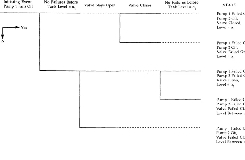
hardware-oriented tree for the system's response to the initiating event "Pump 1 Fails Off" is shown in Figure 2.2. The tree models the different failure modes of the loops explicitly, since these can lead to different system failure modes. Note that since the valve has a larger flow capacity than Pump 2 (see Table 2.2), the valve behavior overrides the behavior of Pump 2 in the first two sequences.

If the dynamics of the system are ignored, the sequences in Figure 2.2 can be

quantified quite simply. For example, the conditional frequency of Sequence 2, given the initiating event, can be approximated by (see Table 2.2)

Fr{Sequence 21 Initiating Event} '==

#v +

Ayr (2.1) where r is time interval since the occurrence of the initiating event. (The last term in the equation represents a scenario in which the valve closes successfully on demand, but later transfers open.)

Overlooking the system dynamics does not affect the failure logic shown in

Figure 2.2. However, it can lead to inaccurate frequency estimates for the two undesired outcomes (dryout and overflow). Further, it prevents the accurate assessment of the frequency distributions for the times to achieve these outcomes. This last piece of information is important, since it indicates the amount of time likely to be available for recovery from the initiating event. These issues are discussed in the following section. 2.2 Event Tree Limitations

To better illustrate the dynamic response of the holdup tank to the initiating event "Pump 1 Fails Off," some of the different possible system response scenarios are shown in Figure 2.3. The scenarios include changes in loop states, failures (denoted by an asterisk), changes in tank level, and changes in the rate of change of tank level (dL/dt). For

example, starting with Box 1, three possible state changes may occur. Either the valve may transfer closed (with rate Ay), Pump 2 may start spuriously (with rate Ap), or the tank level may drop to a, (before either of the two failure events occurs).

Figure 2.3 shows that the behavior of the holdup tank system is fairly complex. This is because of the control laws specified in Table 2.1. These govern the sequence of demands

on the control loops, which in turn, determines the possible sequences of specific failure modes. Thus, the sequences 1 -. 10 -411 -417 and 1 -4 10 -418 lead to two different outcomes

(dryout and overflow, respectively), even though they both involve the sequential failure of Pump 2 and the valve. In the former scenario, the valve fails to close on demand (i.e., the valve is failed open) when the tank level reaches a control region boundary (L = a,),

whereas in the latter, the valve fails closed before a, is reached.

As a result of this complex dynamic behavior, the simplistic quantification of Eq. (2.1) can lead to erroneous results. As an example, the first term in Eq. (2.1) models the likelihood of demand failure for the valve as the frequency that the valve will fail on a single demand. However, scenarios can be easily generated where the valve is demanded more than once. One such sequence of events is: valve closes when L = a,, Pump 2 fails on, valve opens when L = a2, valve fails to close when L = a,. This sequence is partially

represented in Figure 2.3 as the path 1 -+ 2 -+ 3 - 4 - 13 -+ 14. Although a number of events

are involved, it is not very unlikely. Assuming that the demand failure frequency does not change with the number of demands and that the failure time scale is much larger than the time scale for tank level changes, the likelihood of this single sequence is approximately given by

P{sequence} = (1 -

#v).

(1 -

#y) -v

(2.2)

which could easily be of the same order as

#y.

Similar results can be obtained for all other sequences in which the valve eventually fails to close when L = a,. Thus, Eq. (2.1) could be significantly non-conservative.

A second result of neglecting the system dynamics is that the distribution of the times to overflow and dryout cannot be accurately obtained. Consider the sequences 1 -4 10 -+ 18 and 1 - 19 -4 20 in Figure 2.3. Both involve the premature closing of the valve and the premature stopping of Pump 2, and both lead to overflow, but the order of failures is reversed. In the first case, the tank level continues to drop after the failure of Pump 2,

and there is very little time available for the valve to fail. (If the valve doesn't fail in this mode, dryout is likely to occur.) In the second case, the failure of the valve leads to a quasi-stable tank level. Therefore, much longer times to overflow can be expected.

This application shows that a hardware-oriented application of the event tree methodology does not properly quantify the likelihood of the dynamic event sequences, since it does not treat the physical behavior of the system. Further, the event tree cannot be used to determine the distribution of the time to an undesired end state for these sequences.

2.3 Expanded Event Trees

Chapter 1 identifies five different strategies that are often employed (singly or in combination) in an event tree analysis to deal with issues associated with dynamic accident scenarios. These involve the use of: event sequence diagrams, conservative assumptions, top event ordering, event tree modules for different accident phases, and detailed offline

analyses (e.g., for thermal hydraulic plant behavior). A sixth strategy, related to the fourth, is to use a more detailed (i.e., an expanded) event tree.

Typical modifications of the event structure that could lead to better treatment of process variables and time dependence include:

0 explicit inclusion of key values of process variables in top events (e.g. system pressure > 2200 psig),

0 _{treatment of accident phases (including the use of repeated top events),} e use of multiple branches under a top event heading, and

0 treatment of detailed operator actions.

The above modifications have been implemented to some extent in a number of studies. A study of Babcock and Wilcox plants to determine the risk significance of Category C events (i.e., events that require significant safety system and timely operator response to mitigate) has produced a substantially expanded event tree for the loss of feedwater event (see _{Figure 2.4) [28]. The tree treats operator actions (e.g., top events D,}

G, and L) and functional headings in considerable detail. Ref. 28 states that the large tree is useful for providing deeper insights concerning the impact of physical events (e.g., minor overcooling), recovery actions, and cognitive errors. Furthermore, the detail of the tree

allows a reasonable mapping of actual loss of feedwater events into the tree (for use in a precursor analysis).

Other uses of expanded event trees are provided in Ref. 31 (in a human reliability analysis) and in the NUREG-1150 Accident Progression Event Trees (APETs) created for the analysis of events following core damage (e.g., [13]). In the latter case, over 100 top events can be used. Further, there can be more than two branches per top event.

Figure 2.5 shows a portion of a simple expanded event tree created for the holdup tank problem (assuming that the initiating event is the failure of Pump 1). It can be seen that this tree is simply a reformatted version of the diagram provided in Figure 2.3. Figure 2.5, however, is much less compact. It could become extremely large when accounting for the different possible orderings of failure events in different sequences. Conceptually, it is important to note that, unlike Figure 2.3, the expanded event tree does not convey as easily the idea of competing processes. For example, the notion that the first transition to occur following the initiating event is the outcome of three parallel random processes (water level dropping towards a,, valve failure, Pump 2 failure) is much clearer in Figure 2.3.

This is not to say that the expanded event tree cannot be used to solve the problem. As long as the branching frequencies (or "conditional split fractions") are specified

correctly, the sequence frequencies can be properly quantified. For example, consider the first branching shown in Figure 2.5. The frequency that the tank level (L) falls to a, before any failures occur is given by

Fr{L reaches a, before failures} = Fr{(Ti-2 < T 1io) AND (Ti-2 < Ti-19)} (2.3) where the subscripts refer to the transitions shown in Figure 2.3, i.e.,

T1-2 mtime for level to reach a, (assuming no failures)

_L o - a,

TI.10 afailure time for Pump 2 Tj.1g 3failure time for the valve L o initial tank level

4v

rate of level decrease due to open valve

Assuming that the failures of Pump 2 and the valve are independent Poisson processes with rates Ap and Ay, respectively, it can be easily shown that

Fr{L reaches a, before failures} = e-(Ap + Ay)Ti-2 (2.4)

The frequencies of subsequent branches in the tree can be similarly found with only slightly more algebra. Note that, since the distribution for the overall scenario duration is a

desired output, distributions for the transition times must be developed along with the branching frequencies for each scenario.

This discussion shows how event trees can be used to explicitly handle process

variables through expansion (assuming that there is a process variable simulator to update the process variable values). Human actions can be incorporated in expanded event trees in the same manner as used for conventional event trees (e.g., as shown in Figure 2.4). The

scenario history is explicitly represented by the ordering of the top events in the tree structure; this same ordering provides a limited treatment of time progression as well.