HAL Id: tel-00833472
https://tel.archives-ouvertes.fr/tel-00833472
Submitted on 12 Jun 2013HAL is a multi-disciplinary open access archive for the deposit and dissemination of sci-entific research documents, whether they are pub-lished or not. The documents may come from teaching and research institutions in France or abroad, or from public or private research centers.
L’archive ouverte pluridisciplinaire HAL, est destinée au dépôt et à la diffusion de documents scientifiques de niveau recherche, publiés ou non, émanant des établissements d’enseignement et de recherche français ou étrangers, des laboratoires publics ou privés.
a Carbon Nanotube
Jean-Damien Pillet
To cite this version:
Jean-Damien Pillet. Tunneling spectroscopy of the Andreev Bound States in a Carbon Nanotube. Mesoscopic Systems and Quantum Hall Effect [cond-mat.mes-hall]. Université Pierre et Marie Curie - Paris VI, 2011. English. �tel-00833472�
11
Je
an
-Da
m
ien
Pillet
Tu
nn
eli
n
g sp
ec
tro
sc
op
y of
t
he
An
dree
v Bo
un
d S
tat
es i
n
a
C
arbo
n Na
no
tub
e
Jean-Damien Pillet
Quantronics Group
SPEC - CEA Saclay
Tunneling spectroscopy of
the Andreev Bound States
in a Carbon Nanotube
Superconductivity is a fascinating electronic order in which electrons
pair up due to an attractive interaction and condense in a
macroscopic quantum state that can carry dissipationless currents,
i.e. supercurrents. In hybrid structures where superconductors (S)
are put in contact with non-superconducting material (X), electronic
pairs propagating from the superconductor “contaminate” the
non-superconducting material
conferring it superconducting-like
properties close to the interface, among which the ability to carry
supercurrent. This “contamination”, known as the superconducting
proximity effect is a truly generic phenomenon.
The transmission of a supercurrent through any S-X-S structure is
explained by the constructive interference of pairs of electrons
traversing X. Indeed, much as in an optical Fabry-Perot resonator,
such constructive interference of electronic pairs occurs only for
special resonant electronic states in X, known as the Andreev
Bound States (ABS). In the recent years it has been possible to
fabricate a variety of nanostructures in which X could be for instance
nanowires, carbon nanotubes or even molecules. Such devices
have in common that their X contains only few conduction electrons
which implies that ABS are also in small number. In this case, if one
wants to quantitatively understand proximity effect in these systems,
it is necessary to understand in detail how individual ABS form. This
can be seen as a central question in the development of nanoscale
superconducting electronics.
In this thesis, we observed individual ABS by tunneling
spectroscopy in a carbon nanotube.
THÈSE DE DOCTORAT DE
L’UNIVERSITÉ PARIS VI – PIERRE ET MARIE CURIE
ÉCOLE DOCTORALE DE PHYSIQUE DE LA REGION PARISIENNE - ED107 Spécialité :
Physique de la matière condensée
Présentée par Jean-Damien Pillet Pour obtenir le grade de
DOCTEUR de l’UNIVERSITÉ PIERRE ET MARIE CURIE
Sujet de la thèse :
SPECTROSCOPIE TUNNEL DES ETATS LIES D’ANDREEV
DANS UN NANOTUBE DE CARBONE
soutenue le 14 décembre 2011 devant un jury composé de : Vincent Bouchiat (Rapporteur) Juan Carlos Cuevas (Rapporteur) Benoit Douçot (Président du jury)
Silvano de Franceschi Francesco Giazotto
Philippe Joyez (Directeur de thèse)
Thèse préparée au sein du Service de Physique de l’Etat Condensé, CEA-Saclay
N’étant pas de nature particulièrement éloquente, l’écriture de ces remer-ciements représente pour moi un exercice difficile. Néanmoins, je sais à quel point ils sont importants car je dois beaucoup aux personnes qui apparaissent dans ces quelques lignes, et je souhaite leur témoigner la reconnaissance que j’ai pour elles.
La première d’entre elles est bien sûr Philippe. Merci de m’avoir pris en thèse, de m’avoir encadré avec patience et de m’avoir tant appris. Je mesure la chance que j’ai eu de travailler avec un physicien aussi talentueux et pas-sionné. Tu m’as donné l’opportunité de participer à une manip magnifique, et j’ai adoré. Je dois également une fière chandelle à Charis. Ses éclats de rire, sa bonne humeur, sa pêche ont énormément contribué à notre bon travail. Je me rappelle avec beaucoup de plaisir ces longues heures de salle blanche où tu m’expliquais avec pédagogie tes astuces de nano-fabrication. Je m’amusais bien, et je t’en remercie. Lors de ma dernière année de thèse, Marcelo s’est aussi beaucoup occupé de moi, en chantant, en jurant (¡Qué Boludo!), et c’était cool. Tes futur(e)s thésard(e)s ont beaucoup de chance.
Le groupe Quantronique est une grande famille et tous ses membres ont participé à l’agréable déroulement de cette thèse. Je veux les remercier égale-ment. Daniel, tu as toujours su me rappeler avec beaucoup de tact qu’il fallait bosser lors d’une thèse, et ce dès le premier jour (ce qui n’avait pas man-qué de m’intimider, mais fut certainement pour le mieux). Merci également à Hugues dont le second degré m’a souvent décontenancé et également fait beaucoup rire. Ton honnêteté intellectuelle, ta clarté m’ont impressionné et guidé dans ma manière d’aborder la physique. Merci à Cristian qui a plusieurs fois su me redonner du peps à certains moments où je perdais con-fiance, c’était important pour moi et je t’en remercie. Merci à Denis pour ton enthousiasme extrêmement communicatif, et pour tout le temps que tu voulais bien passer avec moi quand je sollicitais ton aide, merci pour ta gen-tillesse. Merci à Patrice (Bertet) pour tes conseils et ton aide. Merci à Pief, pour avoir toujours répondu avec bienveillance à mes questions. Merci à Pascal pour les agréables brins de causette que l’on avait parfois. Merci à
Thomas pour ces moments sympas passés autour d’un café.
Merci aux post-docs du groupe Quantronique que j’ai croisés pendant cette belle aventure doctorale. Francois (Mallet) que j’ai rencontré au début de ma thèse et que j’ai appris à mieux connaitre depuis, avec beaucoup de plaisir. Maciej, you make me discover polish cheese and sausage, I will never forget it. Yui, merci pour les excellents sakés que tu nous ramenais du Japon. Merci Florian, pour toutes ces fois où tu m’as épargné de traverser la forêt pour rejoindre le RER et pour cette sympathique soirée à Dallas. Merci Max de t’être moqué de moi après chaque pot de thèse pour me rappeler la bonne conduite à suivre. Merci Carles, pour ta manière si singulière de parler bonne bouffe et le jabugo de mon pot de thèse. Merci Çağlar pour ta gnac lors de nos parties de foot. Merci également à Romain et Michael. Merci aux thésards avec qui c’était vraiment chouette de vivre cette aventure commune: François (Nguyen), Quentin, Augustin, Andreas, Vivien, Cécile, Olivier... Merci Hélène, tu m’avais transmis l’envie de prendre ta suite lors de ma première visite du SPEC, quel beau cadeau! Landry, tu es bien sûr à part dans cette catégorie puisqu’on est ami depuis longtemps. Je ne saurais pas exprimer ici à quel point j’étais content de te voir arriver dans le groupe. Aussi, j’écrirais simplement que partager avec toi cet intérêt pour la physique c’est énorme.
J’aimerais ajouter à cette liste Fabien pour toutes les heures de Stevie Wonder que j’écoute maintenant grâce à toi, Patrice (Roche) pour m’avoir dit un jour que je n’avais du con que l’air. Thank you Alfredo and Cristina, not only for what you brought to my thesis as theorists, but also because it was really nice learning some physics with you. Thank you Juan Carlos for making us discover, with Landry, the best places to have some tapas in Madrid.
Je remercie aussi tous les autres membres du SPEC qui ont contribué de près ou de loin à cette thèse. Mentionnons Eric Vincent pour son accueil au sein du service, Nathalie Royer, Corinne Kopec-Coelho pour leur aide dans les démarches administratives, et Jean-Michel Richomme pour avoir sauvé mon parquet grâce à sa cire d’abeille.
I would like also to thank the members of my thesis comitee: Benoit Douçot, Vincent Bouchiat, Juan Carlos Cuevas, Silvano de Franceschi and Francesco Giazotto.
Merci aux membres du groupe Qélec du LPA de m’avoir accueilli dans leur groupe après cette thèse pour mon premier post-doc : Philippe, Manu, Nico, François, Benjamin et Michel. C’est une expérience géniale de faire de la physique avec vous, et les lundredi n’ont rien gâché.
Merci à mes potes rencontrés pendant la période de Master car, d’une certaine manière, j’ai fait cette thèse avec eux. Merci Xavier pour ces heures
passées au soleil autour d’une bière, David pour ta méchanceté et ton hu-mour qui ne font qu’un, Philippe d’être un écureuil et pour ces matchs avec le Dynam’eaux, Ludivine pour ces apéros magiques dans ton ancien studio bancale, Loïg d’avoir souffert avec moi aux Buttes et ailleurs, Juliana d’avoir amené la chaleur colombienne à Paris, Yannis de m’avoir emmené parfois au bout de la nuit, Keyan pour ces discussions nocturnes autour d’un bon verre de Bordeaux. Merci à mes potes de l’ENS trop nombreux pour être tous mentionnés mais que je porte dans mon cœur et qui ont vécu cette thèse par procuration : Jérem hockeyeur acquatique, Raph mentor footbalistique, Yo camarade de traquenard, Laura qui illumina la yourte, Romain victime de l’ours blanc, Elsa neo-californienne, Sarah reine du Requin Chagrin, François le petit et le grand, Hélène globe-trotteuse, Oskar toujours chaud pour le ski, Sylvain éleveur d’escargot dans l’âme...
Pour finir, je veux remercier les membres de ma famille. En particulier, mes parents, mon frère et mes deux sœurs, mes grands-parents parce que leur soutien permanent et leur compréhension n’avaient pas de prix. Merci à Jacqueline Campagne pour ton aide lors de la préparation du pot, et pour tes tricots magnifiques. Merci à Cécile parce que tu partages ma vie et que tu me rends heureux.
1 Introduction 13
1.1 Observation of the ABSs . . . 14
1.2 ABSs in Quantum Dots . . . 15
1.3 Perspectives . . . 18
I
Andreev Bound States in Quantum Dots
21
2 Scattering description of the proximity effect 25 2.1 Andreev reflection . . . 252.1.1 Scattering description of AR . . . 28
2.1.2 Case of non ideal materials and interfaces . . . 28
2.2 ABS in S-X-S systems . . . 29
2.2.1 Normal state scattering matrices . . . 29
2.2.2 Andreev scattering . . . 31
2.2.3 Resonant bound states : Andreev Bound States . . . . 31
2.2.4 Supercurrent in S-X-S junctions: contribution of ABSs 32 2.3 ABS in S-QD-S system from the scattering description . . . . 33
2.3.1 Non-interacting dot . . . 33
2.3.2 Weakly-coupled interacting dot: simple effective model 34 2.3.3 Meaning of the sign of the eigenenergies; arbitrariness of the description . . . 36
3 Proximity effects in QD in terms of Greens functions 39 3.1 Effective description of the S-QD-S junction . . . 40
3.1.1 Green’s function of a QD connected to superconduct-ing leads . . . 40
3.1.1.1 Effective Hamiltonian of a S-QD-S junction . 40 3.1.1.2 Green’s function of the Quantum Dot . . . . 42
3.1.2 Tunneling spectroscopy of a QD in terms of GF . . . . 45
3.1.2.1 Definition of the QD’s DOS . . . 45 7
3.1.2.2 Comparison with other type of QD spectroscopy 46 3.1.2.3 Tunneling into ABSs . . . 47 3.1.3 Asymmetric QD . . . 50 3.1.4 Extension of the effective model to a double QD . . . . 51 3.1.5 Supercurrent within the effective model . . . 53 3.1.5.1 Calculation of the supercurrent . . . 53 3.1.5.2 Singlet-doublet transition . . . 56 3.1.5.3 Reversal of supercurrent (0 − π transition)
in a S-QD-S junction: description with our phenomenological approach . . . 57 3.2 Exact treatment of the Quantum Dot with superconducting
leads: the Numerical Renormalization Group . . . 60 3.2.1 Anderson impurity model in NRG . . . 60 3.2.2 Zero vs finite superconducting phase difference across
the QD . . . 62 3.3 Predictions for the DOS of a QD connected to superconductors 63
3.3.1 Modification of the spectral density of a QD upon cou-pling to superconducting contacts . . . 63 3.3.2 Influence of the parameters on ABSs . . . 66 3.3.2.1 Tunable parameters . . . 66 3.3.2.2 Phase dependence: signature of the ABSs . . 66 3.3.2.3 Influence of ΓL, ΓR and U on ABSs “gate
dependence” . . . 68
II
Experimental observation of the Andreev Bound
States
79
4 Description of the samples and measurement setup 83
4.1 Samples description and role of controllable parameters . . . . 83 4.2 Measurement setup . . . 86
5 Tunneling spectroscopy of the Andreev Bound States 89
5.1 Paper “Andreev bound states in supercurrent-carrying carbon nanotubes revealed” . . . 89 5.2 Singlet-doublet transition observed in the TDOS . . . 114
6 Measurement of the flux sensitivity of our devices 119
6.1 Principle of detection . . . 119 6.2 Definition of the flux sensitivity . . . 121 6.3 Setup . . . 121
6.4 Maximization of the flux-tunnel current transfer function dI
dΦ . 122
6.5 Flux noise measurements . . . 123
III
Second experiment: exploring Kondo and
An-dreev Bound States in a Double Quantum Dot
129
7 Proof of Double Quantum Dot behaviour 133 7.1 Charge stability diagram of a DQD . . . 1357.2 Description of the avoided crossings in the stability diagram . 137 7.2.1 Mean-field approximation on the Coulomb repulsion . . 137
7.2.2 Interdot couplings . . . 138
8 Kondo vs superconductivity in single QD 141 8.1 TDOS of an effective single QD . . . 142
8.1.1 Comparison between measurements in the Normal and Superconducting state . . . 142
8.1.1.1 N state measurements . . . 142
8.1.1.2 S state measurements . . . 147
8.1.2 Kondo temperatures . . . 147
8.2 Comparison of the data with NRG calculations . . . 148
9 Specific Double Quantum Dot features 155 9.1 Conventional and split Kondo (CK and SK) in a single effec-tive QD . . . 155
9.2 Strongly coupled QDs: transition from CK to SK . . . 159
9.2.1 Gate-controlled transition . . . 159
9.2.2 Temperature dependences . . . 164
9.3 Weakly coupled QDs: hybridization of two Kondo resonances . 166
IV
Samples fabrication
173
10 Fabrication of a sample 175 10.1 Lithography techniques . . . 17510.1.1 Coating the substrate with resist . . . 175
10.1.2 Exposure . . . 176
10.1.3 Development . . . 178
10.2 Nanotubes growth on Si substrate . . . 178
10.2.1 Substrate characteristics . . . 178
10.2.2 CNT grown by Chemical Vapor Deposition (CVD) . . 178
10.4 Contacting nanotubes with metallic leads . . . 183
10.4.1 Mask fabrication to contact CNTs . . . 183
10.4.2 Metal deposition . . . 183
10.5 Room temperature characterization . . . 189
11 Parameters and techniques for fabrication 193 11.1 Preparation of the resist layers or bilayers . . . 193
11.2 Exposure : parameters and resulting masks after development 193 11.2.1 Parameters of exposure . . . 193
11.2.2 Resulting masks after development . . . 195
11.3 Catalyst preparation and deposition . . . 196
11.3.1 Catalyst suspension preparation . . . 196
11.3.2 Catalyst deposition . . . 197
11.4 Metal deposition and lift-off . . . 197
11.4.1 Description of the electron gun evaporator . . . 197
11.4.2 Lift off . . . 199
V
Appendices
201
A Introduction to Quantum dots 203 A.1 Energy quantization in QDs . . . 203A.2 Hamiltonian description of the system . . . 205
A.3 Weakly coupled QDs . . . 206
A.3.1 Sequential filling . . . 207
A.3.2 Coulomb spectroscopy and Coulomb diamonds . . . 207
A.4 Weakly coupled QDs in a coherent regime : a phenomenolog-ical approach . . . 211
A.4.1 A phenomenological approach . . . 211
A.4.2 Limits of this effective non-interacting model . . . 213
A.5 QDs with stronger coupling . . . 213
A.5.1 Spin-1/2 Kondo effect in nanostructures . . . 214
A.5.2 Variety and universality of the Kondo effect . . . 215
B Quantum dot Green’s function 217 B.1 Definitions of the QD’s GFs and TDOS . . . 217
B.1.1 Green’s functions in real time . . . 217
B.1.2 Retarded and advanced Green’s function in real time . 218 B.2 Matsubara formalism and equation of motion . . . 219
B.2.1 Notation in Matsubara imaginary time . . . 219
B.2.3 Equation of motion . . . 220
B.3 Calculation of the QD’s GF by resolution of the EOM . . . 220
B.3.1 Resolution of the EOM . . . 221
B.3.2 Calculation of the QD’s self-energy . . . 222
B.3.3 Comment on the temperature dependence of the QD’s GF . . . 223
B.3.4 Poles as roots of the inverse GF’s determinant . . . 223
B.3.5 Physical signification of a GF . . . 223
B.4 Useful identities for calculation of the tunnel Density of states and supercurrent . . . 225
B.4.1 Lehmann representation . . . 225
B.4.2 Relation between lesser, greater, advanced and retarded GFs at equilibrium . . . 226
C Relation between ABS’s energies and Josephson current 229 C.1 Josephson current carried by a S-QD-S junction . . . 229
C.1.1 Symmetrization of the current GF . . . 230
C.1.2 Expression of the current GF . . . 231
C.2 Supercurrent carried by the ABSs . . . 233
C.3 Supercurrent carried by the continuum . . . 235
D Tunneling spectroscopy 239 D.1 The tunnel current and tunnel density of states . . . 240
D.1.1 Description of the system and tunneling Hamiltonian . 240 D.1.2 Calculation of the tunnel current . . . 241
D.1.2.1 Definition of the tunnel current operator . . . 241
D.1.2.2 Calculation of the tunnel current using the Kubo formula . . . 242
D.1.2.3 Tunnel differential conductance . . . 244
D.2 Broadening of the ABSs due to the coupling to the tunnel probe244 D.2.1 ABSs coupled to a normal tunnel probe . . . 244
D.2.2 ABSs coupled to a superconducting tunnel probe . . . 246
D.3 Extracting the Density of States (DOS) from the differential conductance . . . 247
D.3.1 Principle of the deconvolution procedure . . . 248
D.3.2 Introduction of a Dynes parameter . . . 250
D.3.3 Influence of the finite measurement range . . . 250
E Calculation of Coulomb blockade peaks for a DQD 251 E.1 GF of an interacting DQD connected to normal leads . . . 252
E.1.2 Interacting DQD’s GF calculation . . . 253 E.2 Self-consistent calculation of the DQD’s occupancy and TDOS 255 E.2.1 Self-consistency . . . 255 E.2.2 DQD’s TDOS . . . 256
F Bogoliubov de Gennes equations formalism 259
F.1 Inhomogeneous superconductivity . . . 259 F.1.1 Effective Hamiltonian describing an inhomogeneous
su-perconductors . . . 259 F.1.2 Bogoliubov-de Gennes equations . . . 260 F.1.3 Interpretation of the BdG equations as ’one-particle’
wave equations . . . 261 F.1.4 Arbitrariness of the description and diagonalization with
a different spinor . . . 262 F.1.4.1 Arbitrariness of the description . . . 262 F.1.4.2 Same physics described . . . 263 F.1.4.3 Diagonalization using a spinor with
equiva-lence between the spins . . . 264 F.1.4.4 Excitation picture . . . 266 F.2 States in gap . . . 267
G Andreev Bound States in a well-known system 269
G.1 ABSs in an infinitely short perfectly transmitted one dimen-sional single channel . . . 269 G.2 ABSs in an infinitely short one dimensional single channel with
Introduction
Superconductivity is a fascinating electronic order in which electrons pair up due to an effective attractive interaction and condense into a state, char-acterized by a macroscopic phase, that can carry dissipationless currents,
i.e. super currents. It was observed and understood for a long time that in
hybrid structures where superconductors (S) are put in contact with non-superconducting materials (X), electronic pairs propagating from the su-perconductor “contaminate” the non-superconducting material conferring it superconducting-like properties close to the interface, among which notably the ability to transmit supercurrent. This “contamination”, known as the su-perconducting proximity effect was gradually understood to be truly generic: whatever the electronics properties of X, proximity effect will occur, albeit possibly only on a range of the order of the interatomic distance in unfavor-able cases.
The transmission of a supercurrent through any S-X-S hybrid structure is explained by the constructive interference of pairs of electrons traversing X. Indeed, much as in an optical Fabry-Perot resonator, such constructive inter-ference of electronic pairs occurs only for special resonant electronic states confined inside X, known as the Andreev Bound States (ABS). Reciprocally, knowing the properties of the ABS is enough to characterize the supercon-ducting properties of the S-X-S structure.
In hybrid nanostructures containing many ABSs, a statistical knowledge about the ABSs provided by quasiclassical theories suffices to predict the su-percurrent in the structure. This is the case for instance in Superconductor-Normal metal-Superconductor (S-N-S) microbridges. However, in the recent years its has been possible to fabricate a variety of hybrid nanostructures in which X could be for instance semiconducting nanowires [1, 2, 3], carbon nanotubes [4, 5, 6, 7, 8, 9, 10, 11], aggregates [12, 13, 14] or even molecules [15]. Such devices have in common that their X contains only few conduction
electrons which implies that ABS are also in small number. In this case, if one wants to quantitatively understand proximity effect in these systems, it is necessary to understand in detail how the individual ABS form in such device for which quasiclassical methods are ineffective. This can be seen as a cen-tral question in the development of nanoscale or molecular superconducting electronics.
In a first step to address this question, the initial goal of this thesis work was to observe individual ABSs in a system expected to contain only a few of them. To do so, we have set up an experiment with an hybrid device in which X was a carbon nanotube (CNT). In such a structure, it was indeed expected that there would be only a small number of ABS that one could resolve individually by performing tunneling spectroscopy directly on the CNT.
When wanting to understand the formation of ABS in systems with few electrons, one is rapidly faced with the question of Coulomb interaction: in contrast to the (quasi-)electrons of the superconductor that experience an effective attractive interaction, in a nanoscale X with few electrons, Coulom-bian repulsion is expected to play a large role. Hence a second question one has to address is: how do ABSs form in a system with Coulomb repulsion (obviously opposing superconducting pairing)? Prior to this thesis work, many theoretical works had addressed this point, but there had been no ex-perimental counterpart taking the point of view of the ABS formation. Our experimental results shed light on the effect of Coulomb repulsion on ABSs.
1.1
Observation of the ABSs
The concept of ABSs has been widely used to understand a large panel of experiments in hybrid nanostructures. Yet, no experiment had so far allowed a detailed and direct spectroscopy of the ABSs. In this thesis work, we report the first spectroscopy of individually resolved ABSs, in a CNT-based hybrid device.
CNTs are suitable to perform the spectroscopy of ABSs, first, because as already mentioned they should host only a reduced number of ABSs when contacted to Ss. Also, establishing good contacts to superconducting leads has already been demonstrated [4, 7, 8], and they have a favorable elongated geometry providing an easy access to a tunnel probe. In our setup the CNT is contacted to aluminum electrodes distant of 0.7 µm. These electrodes become superconducting below ∼ 1K and “contaminate” the CNT. As elec-trodes are reconnected, they form a loop. This geometry permits to impose a superconducting phase difference δ across the CNT by threading a
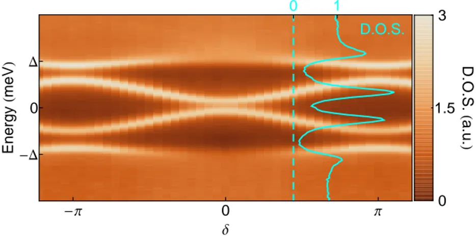
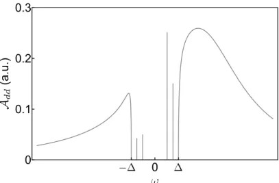
mag--Π 0 Π -D 0 D 0 1 ∆ Energy H meV L 0 1.5 3 D .O .S . H a .u . L D.O.S.
Spectroscopy of the Andreev Bound States
Figure 1.1: Colorplot of the density of states (D.O.S.) of a CNT measured as a function of the superconducting phase difference δ between electrodes. Andreev Bound States appear as resonances (bright lines on this graph) whose energies depend periodically on δ. The solid trace corresponds to a cross-section of the data at the phase indicated by the dashed line.
netic flux in the loop. In between these electrodes, a tunnel probe is weakly contacted to the CNT in order to measure its density of states by tunnel-ing spectroscopy. The detailed description of our process of fabrication is exposed in part IV.
In part II, we present a first experiment realized on such structure in which we have successfully observed individual ABSs in the CNT. They appear as resonances in the density of states of the CNT within a gap of width 2∆ where ∆ is the amplitude of the order parameter of the superconducting electrodes (see Fig. 1.1). We were also able to measure the 2π-periodic dependence with
δ of the ABSs’ energies. This phase dependence is a signature of the ABSs
and is intimately related to their role in the transport of supercurrent in the CNT, even though that current was not actually measured in the experiment. The supercurrent carried by an ABS is indeed given by the derivative if its energy with respect to δ. In chapter 6, based on this behaviour, we evaluate the performance of our device as a SQUID-magnetometer.
1.2
ABSs in Quantum Dots
Trying to interpret this first experiment has led us to address the question of the formation of ABSs in Quantum Dots (QDs). This is because, most experiments involving electronic transport through CNTs can be interpreted
-11.7 -11.4 -11.1 -D 0 D VbgHVL Energy H meV L 0 3 6 D .O .S . H a .u . L -11.7 -11.4 -11.1 -D 0 D VbgHVL Energy H meV L 0 1 2 D .O .S . H a .u . L
Figure 1.2: Experimental (upper graph) and theoretical (lower graph) de-pendence of the Andreev Bound States spectra with the voltage applied on a back gate. Comparison of our experimental results and calculations per-formed within the phenomenological approach of Ref. [16] yields a very good agreement. In this model, ABSs appear as facing bell-shaped resonances with their bases resting against opposite edges of the superconducting gap. For large enough Coulomb repulsion these resonances may form a loop. The features observed in experimental data can be identified as such bell-shaped resonances corresponding thus to different orbitals in the nanotube. Closer inspection reveals however that adjacent resonances are sometimes coupled, forming avoided crossings, so that we need to consider the case where two orbitals contribute simultaneously to the spectral properties within the su-perconducting gap. For this, we extend the model to two serially-connected QD each containing an orbital, with a significant hopping term in between. This model is fairly natural, given that the centre tunnel probe electrode is likely to act as an efficient scatterer.
in terms of QD, and ours in no exception. In QDs, the electronic structure, prior to the connection to superconducting leads, is quantized in orbitals that can each contain two electrons of opposite spin, and a gate electrode allows to control the filling of these orbitals. Moreover, due to Coulomb repulsion, the energy necessary to add an electron to the QD the charging energy -is one of the biggest energy scale of the system. In our experiments it -is ten times larger than the characteristic energy of superconductivity ∆.
Our experiment showed that by applying a voltage on a capacitively cou-pled gate, one can tune the ABSs’ energies. The observations were consistent with ABSs arising from the hybridization of levels of opposite spin belong-ing to orbitals of the CNT behavbelong-ing as a double quantum dot. In part I, we introduce the theoretical approaches which allow to describe these ex-perimental results. A first approach is based on an effective non-interacting model developed in Ref. [16] by Vecino et al. It consists in a phenomenolog-ical treatment - Hartree-Fock like - of the Coulomb repulsion in the CNT. Though based on rough approximations, this approach yields a rather good agreement with experimental results (see Fig. 1.2) allowing to extract de-tailed information on our sample: couplings between CNT and the leads or strength of Coulomb repulsion. Spectra of ABSs constitute thus a powerful spectroscopic tool for QDs. We validate this phenomenological approach, for the parameters range of our experiment, by comparison with exact numerical renormalization group (NRG) calculations.
In part III, we report on a second experiment that aimed at filling the gaps left in the analysis of the first experiment. In particular we wanted to check the double-dot analysis that we had used for the first experiment. A second goal of this experiment was to investigate the possible interplay between the PE in a QD and the Kondo effect. The Kondo effect is complex many-body phenomenon which arises in a QD connected to normal leads (i.e. non superconducting). When the QD contains, in its last occupied orbital, a single electron, its spin degree of freedom interacts with conduction seas of the electrodes. Virtual charge fluctuations, in which an electron briefly migrates off, or into the QD lead to spin-exchange between the local moment and the conduction sea [17]. This spin-exchange gives rise to the formation of a many-body spin-singlet state characterized by an energy scale TK: its
Kondo temperature. This state manifests by a peak at the Fermi level in the density of states of the CNT. Its interplay with superconductivity has been the subject of numerous experimental [5, 9, 14, 18, 19, 20, 21] and theoretical works (see for example [22, 23, 24, 25]). There are however still few quantitative experimental investigations leaving many open questions, like: is there an interplay between Kondo effect and superconductivity ruled by the ratio TK/∆? We explored this interplay through the spectroscopy of
ABSs by comparing normal state and superconducting state measurements of the CNT’s density of states (see Fig. 1.3). Our experimental results show that, within the parameters range of our experiment, Kondo effect observed in the normal state induces no qualitative change in the behaviour of ABSs. The behaviour that we observe experimentally is well described by NRG calculations which can capture both the Kondo effect and the formation of ABSs in QDs, as is shown in Fig. 1.3. We also discuss the quantum transition between a spin-singlet and a spin-1/2 ground state of the QD in the superconducting state when the gate voltage is varied. The most spectacular effect of such transition is the reversal of the supercurrent by adding a single extra electron in the QD. This is directly visible in our spectroscopy by an ABS that crosses the Fermi level in forming a loop pattern as a function of the gate voltage in an odd valley of the QD. A second signature of this transition is a phase shift of π in the phase-dependence of the ABSs, indicating that the CNT goes from a zero to a pi-junction behaviour. Finally in this second experiment we show some spectroscopic features that are specific of double-QD physics.
1.3
Perspectives
Our observation of the ABSs in a CNT constitutes an important step forward in the exploration of PE in nanostructure. This experiment is not just the confirmation of a fifty years old prediction [26, 27, 28], but is at the heart of modern issues on hybrid nanostructure with superconducting leads. This field is presently very active. People are considering all sorts of S-X-S de-vices with all possible electronic properties for X, and some of them are very promising. For instance, if X is a topological insulator (or a semiconductor with strong spinorbit coupling and Zeeman splitting), it is predicted that -under appropriate circumstances - some ABSs should take the appearance of Majorana fermions which could be a basis for the implementation of topolog-ical quantum information processing. But so far, only a limited number of predictions have considered the effect of interactions [29]. Our work should give some insight in order to picture the influence of interaction on the for-mation of Majorana fermions. Apart from this exciting perspective, other cornerstone experiments could extend the present work.
Semiconducting nanowires (NW) are characterized by a large spin-orbit interaction and can be contacted to Ss. Since they share similar geometry than CNTs, the spectroscopy of ABSs could, in principle, be realized in the same way than in our experiment. Such spectroscopy would open exciting perspective for the understanding of the interplay between superconductivity
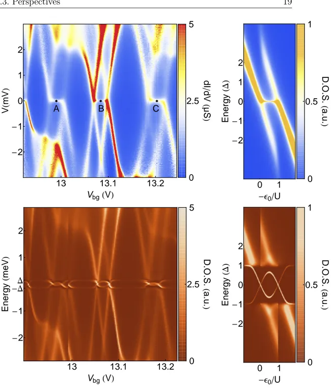
ì ì ì 13 13.1 13.2 -2 -1 0 1 2 VbgHVL V H mV L 0 2.5 5 dI dV H µ S L A B C 1 0 0 -2 -1 1 2 -Ε0U Energy HD L 0 0.5 1 D .O .S . H a .u . L 13 13.1 13.2 -D D -2 -1 1 2 VbgHVL Energy H meV L 0 2.5 5 D .O .S . H a .u . L 1 0 0 -2 -1 1 2 -Ε0U Energy HD L 0 0.5 1 D .O .S . H a .u . L
Figure 1.3: On the left: densities of states of the CNT measured as a function of the gate voltage Vbg when the leads are driven into their normal state with
a magnetic field (upper graph), and when they are in their superconducting state (lower graph). In normal state measurements, Kondo peaks (indicated by black diamond) appear at the Fermi level. In the superconducting state, these peaks disappear because of the opening of a superconducting gap be-tween −∆ and +∆. Within this gap, ABSs appear because of proximity effect. They form loop when we tune the gate voltage Vbg. All these
be-haviours are nicely captured by NRG approach, as shown by the matching graphs on the right.
and spin orbit interaction.
Some two-dimensional electron gases (2DEG) in semiconductor heterostruc-tures are also characterized by a strong spin orbit [30, 31]. Hence, they were also proposed as candidate for the observation of Majorana fermions [32]. Moreover, the possibility of patterning the 2DEG and introducing lateral gates offer an even richer degree of control than CNTs or NWs: couplings to the leads as well as charging energies would be tunable parameters, in contrast to our experiment where they are essentially imposed during fabri-cation of the device. Moreover, as coupling between the tunnel probe and the QD could also be tuned, it would make possible to limit the broadening of ABSs due to the coupling to the probe, thereby increasing the resolution of Andreev Bound States spectra as a spectroscopic tool. We could also, as in Ref. [33], realize this spectroscopy through an extra QD acting as an energy filter and reach an even better resolution.
Andreev Bound States in
Quantum Dots
Superconducting proximity effect and Josephson effect Close to an interface with a superconductor (denoted by S), materials that are not in-trinsic superconductors (hereafter called normal materials and denoted by X) acquire some characteristic properties of the superconductor. This effect, generically known as “the proximity effect”, is of wide generality although its strength and length-scale depend on the electronic properties of the normal material and on the quality of the interface.
A striking manifestation of this proximity effect can be observed in S-X-S junctions: if X is thin enough and the temperature low enough, such a junction can sustain a supercurrent. Such phenomenon constitutes a general-ization of the supercurrent flow through an insulating barrier (S-I-S junction) described by B. Josephson, and, by extension, it is also called Josephson ef-fect.
The physics of the proximity effect was investigated and understood soon after the discovery of the BCS theory. The group led by de Gennes in Orsay notably contributed to this work [27, 34, 35].
With the advent of mesoscopic physics there was a renewed interest on the proximity effect that started in the 90’s. This revival was pushed both by the development of microfabrication techniques that allowed to make elabo-rate heterostructures at the scales relevant for the proximity effect, but also by the emergence of new ideas in the domain of mesoscopic physics, such as the Landauer-Büttiker scattering formalism [36], Random matrices [37], Nazarov’s circuit theory [38], etc...
This has led to consider proximity and Josephson effects in countless structures, where X could be anything among molecules (graphene, carbon nanotube, fullerene), diffusive normal metals, ferromagnetic materials, semi-conductors (two dimensional electron gas or nanowires) and atomic contacts. In the recent years the introduction of new materials has made the field of proximity effect richer with for instance the observation of a striking µm-range proximity effect though ferromagnetic layers presumably due to equal-spin Cooper pairs (a.k.a. “equal-spin-triplet”) [39, 40, 41], or predictions of the presence of composite “Majorana fermions” in exotic proximity structures involving topological insulators or semiconductors with strong spin-orbit cou-pling [42].
The behaviour of all the above mentioned structures, despite their very different electronic properties, can be qualitatively understood within a re-markably uniform language based on key concepts of the superconducting proximity effect: Andreev reflections and Andreev bound states [26, 28, 43]. These two concepts are easily understood and depicted in the com-bined framework of the Landauer-Büttiker scattering formalism and the Bogoliubov-de Gennes formulation [44] of the BCS theory [45, 46, 47]. We
first introduce them below.
Then we will restrict the topic to proximity effect in Quantum dots (a general introduction to Quantum Dots is provided in appendix A). Many experiments have already reported the measurement of a Josephson super-current through QDs [48], but the link between these observations and the underlying phenomena remained rather qualitative. By addressing the DOS of the QD in proximity effect, we reach a deeper understanding of these experiments.
In chapter 2, we will introduce the concepts of Andreev reflection and Andreev Bound States with scattering formalism which provides intuitive pictures of those notions. Afterward, in chapter 3, we will introduce a Green’s function description of the superconducting proximity effect in QD. This formal tool affords a handy and straightforward way to calculate observables in a QD. In this part of the thesis, we will first focus on not too strongly coupled QD in which effective non-interacting models are appropriate. Later on, we will address the case of QD displaying Kondo effect [49].
Scattering description of the
proximity effect
In the present chapter, we adopt the scattering approach to describe general properties of the proximity effect. This approach, pioneered by C. Lambert [50] and C. Beenakker [51], allows to obtain the quasiparticle excitation spec-trum of a Josephson junction including the Andreev Bound States. From this spectrum can be deduced various observables such as the supercurrent.
Here, we follow closely Beenakker’s method and notations to introduce the process of Andreev reflections and the formation of Andreev Bound States in S-X-S junctions. Finally, since the experiments we performed use a carbon nanotubes as a QD, we eventually apply this description to a quantum dot in which interactions are treated in a minimal fashion.
2.1
Andreev reflection
Andreev reflection is the process by which charge carriers from a normal metal (X) can enter a superconductor (S). Addressing this problem amounts to solve the Bogoliubov-de Gennes equations at an X-S interface, and this is a difficult problem since one should in principle determine the superconducting order parameter ∆ (see appendix F for definition) self-consistently while solving the equations. Fortunately, in many experimental situations where a weak link is connected to much more massive superconducting electrodes, approximating the order parameter as a step function at the interface yields a simple and yet very good approximation. In this case, the Andreev reflection amplitude can be obtained by simply matching wave functions of the normal metal with those of the bulk superconductor.
Let us consider an electron in the normal metal (x < 0) at an energy 25
E
Δ
- Δ
x
x = 0
DOS of the S part EF E < ΔX
S
x
x = 0
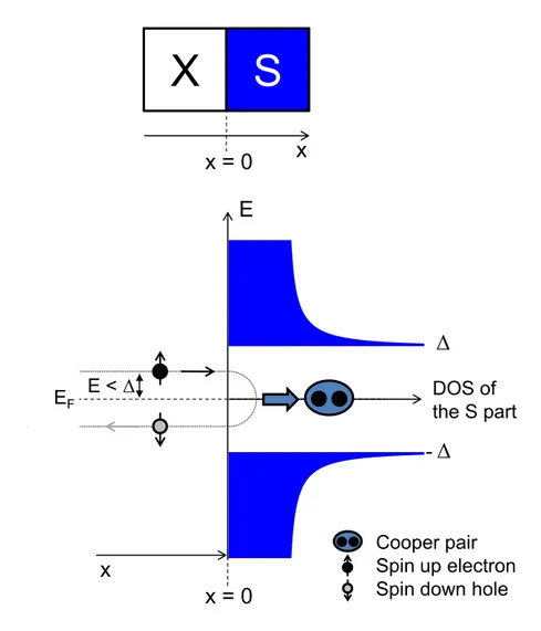
Cooper pair Spin up electron Spin down holeAndreev Reflection of an electron into its time-reversed conjugated hole at a X-S interface
Figure 2.1: Schematic representation (bottom diagram) of the Andreev re-flection of an electron into its time-reversed conjugated hole at a X-S in-terface. The latter is represented in the top diagram with the X part on the left and the S part on the right. When a right-moving spin up electron in the X part, with an energy E smaller than the superconducting gap ∆, reaches the interface with a S part (represented by its density of states in blue) at x = 0, it cannot enter by itself the superconductor. It may be either normally reflected (if the interface is not perfect) or Andreev reflected into its time-reversed conjugated hole (left-moving and spin down). In the latter case, a Cooper pair is transferred to the superconductor S.
(defined with respect to the Fermi level EF) lower than the superconducting
gap |ϵ| < ∆ propagating toward the superconducting part (x > 0). Since the solutions to the BdG equation in the superconductor (equivalent of the Schrödinger’s equation in normal materials) are in the Nambu space, we also describe the normal metal states in this space. The incident electron is then
a state: [
1 0
] eikx
that we need to match to states in the S region (see Eq. F.7 of section F.2 in appendix F) at the interface (x = 0 see Fig. 2.1). For matching the hole part, it is necessary to introduce a reflected hole component on the N side (l.h.s.): [ 1 0 ] eikx+ λ [ 0 1 ] eikx = µ [ 1 a(|∆|ϵ )e−iϕ ] eik+(ϵ)x
where λ and µ are coefficients to be determined (one rapidly sees that µ = 1) and a is a function of the energy given by the ratio of the coherence factors (see appendix F). Since |ϵ| < ∆, the wavevectors are imaginary on the S side (r.h.s.) and only the evanescent wave (Im [k+(ϵ)] > 0) is an acceptable
physical solution. The hole reflection amplitude is simply:
λ = a ( ϵ |∆| ) e−iϕ
For|ϵ| < ∆, one has |a|2 = 1 so that, the electron is reflected as a hole with unit probability (|λ|2 = 1). Note that the phase of reflected hole relative to that of the incident electron depends both on energy (through arg(a)) and on the phase ϕ of the order parameter of the superconductor (see Fig. F.3). A hole in X incident on S is conversely reflected as an electron. However, a hole propagating to the right has a negative wave vector and has to be matched with a −k−(E) solution. The reflection coefficient is then a(|∆|ϵ )e+iϕ, where
ϵ is the energy of the reflected electron.
This is the Andreev reflection process that explains how charges pass from N to S: the right-propagating incident electron carries a charge −e, and it is reflected as a left-propagating hole of charge +e. By conservation, a charge−2e has to enter the superconductor as a Cooper pair, in the so-called "superconducting condensate".
The Andreev process is not restricted to|ϵ| < ∆; the same reasoning can be made at all energies in exactly the same way, with the same formal result: the a function correctly gives the probability amplitude for the hole reflection
process at all energies. Thus the a function is generally called the Andreev reflection amplitude. As shown in appendix F (Fig. F.3), for |ϵ| > ∆, the Andreev reflection probability is less than unity, falling off rapidly away from the gap edge.
2.1.1
Scattering description of AR
From the point of view of electrons and holes in the normal metal, one can describe the Andreev reflection process using a scattering matrix, that relates the amplitudes of the incoming states on the NS interface and outgoing (reflected) states: ( eout hout ) = a ( ϵ |∆| ) ( 0 e−iϕ eiϕ 0 ) ( ein hin )
This scattering matrix is unitary (i.e. particle-number conserving) only for energies|ϵ| < ∆. At larger energies, propagating quasiparticles can enter the superconductor and Andreev reflection is only partial.
2.1.2
Case of non ideal materials and interfaces
The above description of plane wave matching to describe the Andreev re-flection is not essential. The process also occurs in diffusive materials, and the Andreev reflection amplitude is exactly the same for diffusive states, as long as the inverse proximity effect can be neglected.
In cases where the inverse proximity effect cannot be neglected, the or-der parameter has a spatial dependence different from a step function at the interface. Then one cannot simply match the wave functions of the N side with the bulk superconductor wave functions. However the fact that no propagating states exist in S at energies |ϵ| < ∆ is still true, so that full Andreev reflection remains exactly valid. The only change will be that the detailed energy dependence of the AR amplitude will be quantitatively different from that given above, but not qualitatively. Hence, whatever the interface, whatever the materials, AR remains perfect and can be seen as a spectral property of NS interfaces.
For interfaces with imperfect transparency, a normal (non-Andreev) scat-tering also occurs at the interface, partly reflecting electrons as electrons and holes as holes, in addition of the AR process. Both these processes can be cast into a single scattering matrix that remains unitary at energies below the gap. The normal scattering process can also be formally separated from the pure AR process. This is what we do in the following.
2.2
ABS in S-X-S systems
The Landauer description of coherent conductors [36] (Fig. 2.2) in the nor-mal state allows to describe transport in terms of independent channels, the Landauer channels. This picture, valid in absence of electron-electron and inelastic interactions inside the device, elegantly deals with interferences in quantum devices and yields a powerful and intuitive description of such sys-tems. This approach can be adapted to describe systems with superconduct-ing reservoirs provided we can neglect the pairsuperconduct-ing interaction in the central part of the device, that is, when the scattering of electrons and of holes can be considered separately. This assumption is justified if either the central part is not intrinsically superconducting (the pairing interaction is zero inside the central part), or the central part is much shorter than the coherence length of superconductor so that the pairing interaction has a negligible weight in that part compared to the reservoirs. Moreover, as in Ref. [51], we assume that the only scattering in the superconductors consists of Andreev reflection at the SN interfaces, i.e. normal scattering happens only within the central part of the device.
We first write the scattering matrix for electrons and holes in this system in the normal state.
2.2.1
Normal state scattering matrices
For electrons in the central part, the vectors of incident (a) and reflected (b) electronic modes in the left (n1 modes) and right (n2 modes) leads are related by the scattering matrix according to:
( be n1 ben2 ) = Se. ( ae n1 aen2 )
where Se, the scattering matrix, a priori depends on energy and has the block
structure: Se= Se(ϵ) = ( r(ϵ) t(ϵ) t′(ϵ) r′(ϵ) )
Left
reservoir
(n1 modes)
Right
reservoir
(n2 modes)
S
eS
hScatterer
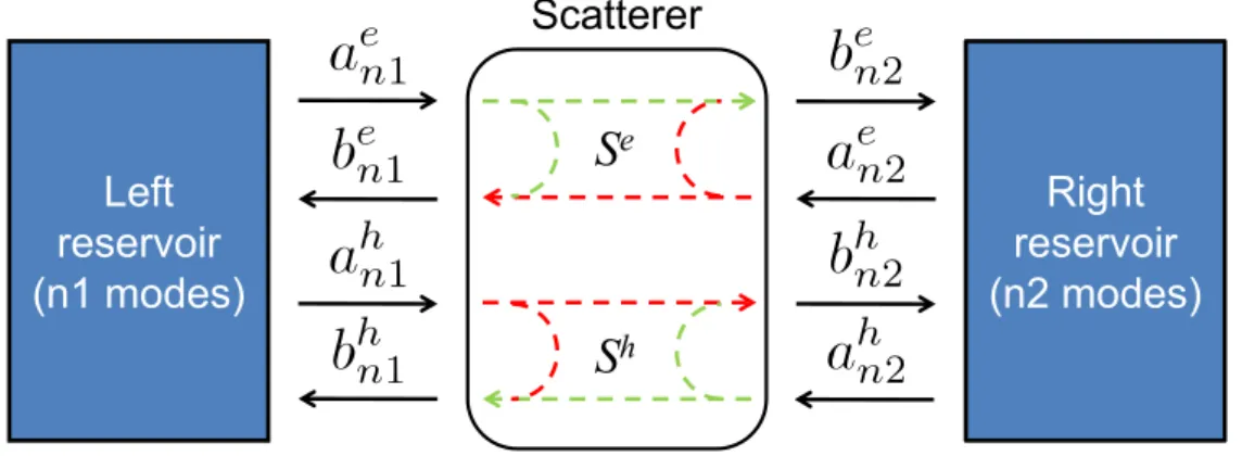
Figure 2.2: In the Landauer description, a coherent conductor is described by a matrix SN =
(
Se 0
0 Sh
)
containing the probability amplitudes for a mode of a reservoir to be either reflected or transmitted.
(in systems obeying time-reversal symmetry1 t′ = t). Similarly, the hole scattering is given by:
( bhn1 bh n2 ) = Sh. ( ahn1 ah n2 )
For a given electron at energy ϵ (relative to EF), its conjugated hole
in Nambu space has opposite energy. In systems where electron and hole components of the Nambu space inside X have the same symmetries as BCS superconductors (that is, all states are spin-degenerate and holes are exact time-reversed symmetric particles of electrons), the scattering of holes can be obtained simply by “projecting the electron movie in reverse motion”. In that case the Se and Sh matrices for holes and electrons are linked by:
Sh(ϵ) = (Se(−ϵ))∗
Combined scattering of electrons and holes on X can thus be expressed
1In mesoscopic physics, a time-reversal symmetry is considered to be broken when par-ticles with opposite spins going in opposite directions have different amplitude probability to be transmitted, for example in presence of a magnetic field. However time-reversal symmetry, in the sense of particle physics, is of course not broken: if we really reverse time, we also reverse magnetic field and a particle will go over the same trajectory, simply reversed.
as: be n1 be n2 bhn1 bh n2 = SN. ae n1 ae n2 ahn1 ah n2
where SN can be cast as a block matrix:
SN =
(
Se 0
0 Sh
)
with 0 a matrix with all its entries equal to 0.
2.2.2
Andreev scattering
As shown above in section 2.1.1, the Andreev reflection can be described as a scattering process for which the b states become incident and the a are
emergent: aen1 ae n2 ah n1 ahn2 = SA. ben1 be n2 bh n1 bhn2
where SA can also be cast as a block matrix:
SA = a ( ϵ |∆| ) 0 In1e −iϕ1 0 0 In2e−iϕ2 In1eiϕ1 0 0 In2eiϕ2 0
where In is a n× n identity matrix and ϕ1 and ϕ2 are the superconducting
phases of the two reservoirs.
2.2.3
Resonant bound states : Andreev Bound States
Cascading the above SN and SAmatrices, an incident state ain =( ae
n1aen2ahn1ahn2
)
is stationary and bound inside X (with only evanescent tails into the su-perconductors) whenever ain = SA.SNain. This condition implies that the
energies which give the roots of the equation2:
Det [I− SA.SN] = 0 (2.1)
are the energies of these bound states. These states mediated by the An-dreev reflection are the so-called ABSs. Therefore, if X is described by an appropriate scattering matrix SN, the ABSs energies can always be found
with relation 2.1. The existence of Andreev Bound States is thus a universal feature of hybrid S-X-S junction3.
Beenakker and van Houten pointed out [52] that this situation was analo-gous to a Fabry-Perot optical resonator with phase-conjugating mirrors. The role of the optical cavity is played by the coherent conductor, a CNT in our experiment, and its interfaces with superconducting leads play the role of the mirrors. Andreev reflection is analogous to optical phase conjugation: an electron in the nanostructure with energy below the superconducting gap is reflected as its time-reverse conjugated hole. This hole can be subse-quently reflected as an electron, and if the phase acquired during this cycle fulfils a resonant condition, ABSs form. ABSs thus correspond to optical resonant standing waves, being however electronic excitations constituted by a superposition of time-reversed states with opposite spins. Within the superconducting gap, ABS form a discrete spectrum which depends on the superconducting phase difference δ = ϕ1 − ϕ2 between the left and right
superconducting electrodes, as we can see by rewriting Eq. 2.1 in the form: Det I − a ( ϵ |∆| )2( e−iδ2 0 0 eiδ2 ) Se(ϵ) ( eiδ2 0 0 e−i2δ ) Sh(ϵ) = 0
This phase dependence is the manifestation of the fact that in each AR the electron (resp. hole) acquires a phase4 ϕ
1 or ϕ2 (resp. −ϕ1 or−ϕ2), such that
after a cycle the phase acquired depends on δ. The phase difference is thus analogous to the length of the optical Fabry-Perot. This phase dependence is a characteristic signature of the ABSs in S-X-S structures and the proof that they carry supercurrent (see 3.1.5, appendix C and Ref. [51, 53, 54]).
In appendix F, we discuss the well-known case of an infinitely short single channel with perfect and finite transmission.
2.2.4
Supercurrent in S-X-S junctions: contribution of
ABSs
The scattering formalism is not restricted to the extraction of the ABSs’ spectrum. Beenakker has indeed shown in Ref. [54] the link between the
3It is also true for S-X structures where bound states can form at interfaces. In this case the ABSs’s energies don’t depend on the phase.
4Not only, as it also acquires an energy-dependent phase arg(a(E |∆|
))
in each AR, and also a phase due to propagation and scattering in the coherent conductor.
spectrum of a S-X-S junction and the supercurrent flowing through it. He decomposes the latter in two parts:
• the contribution of the ABSs which is related to the derivative of their energies with respect to δ,
• and the contribution of the continuum (for |E| > ∆).
He shows in particular that for the case of a quantum point contact, the second contribution is negligible and all the supercurrent is carried by the ABSs.
In appendix C, we give an alternative demonstration, for the case of a Quantum Dot, of these physical properties using Green’s function techniques.
2.3
ABS in S-QD-S system from the
scatter-ing description
We now consider the case where the central scatterer is a quantum dot (QD). In a QD, scattering occurs via resonant tunneling through discrete states.
2.3.1
Non-interacting dot
If we consider, as a first approach, that electrons do not to interact in the QD, the lead-QD-lead structure can be modelled as a double barrier system. The energy levels are then discrete spin-degenerate states given by the ladder of waves-in-a-box solutions to the Schrödinger equation.
Let ϵr be the energy of one of these resonant levels, relative to the Fermi
energy EF in the reservoirs, and let ΓL/~ and ΓR/~ be the tunnel rates
through the left and right barriers. We denote Γ = ΓL+ΓR. If Γ≪ ∆E (with
∆E the level spacing in the quantum dot) and T ≪ Γ/kB, we can assume that
transport through the QD occurs exclusively via resonant tunneling through the spin degenerate level of energy ϵr. The conductance G of the QD has
thus the form[55, 56, 57]:
G = 2e 2 h 4ΓLΓR ϵ2 r + Γ2 = 2e 2 h TBW (2.2)
where TBW is the Breit-Wigner transmission probability at the Fermi level.
Assuming the resonance couples to a single mode in the reservoirs (general-ization to many modes is straightforward, see Ref. [58]), the normal-state
Breit-Wigner scattering matrix sϵr(ϵ) which yields this conductance has the form [56]: sϵr(ϵ) = ( 1− i2ΓL ϵ−ϵr+iΓ ) ei2δL −i √ 4ΓLΓR ϵ−ϵr+iΓ e i(δL+δR) −i√4ΓLΓR ϵ−ϵr+iΓe i(δL+δR) ( 1− i2ΓR ϵ−ϵr+iΓ ) ei2δR (2.3)
Note that since the reflection phases δL and δR later vanish in the
determi-nation of the energies of the ABS, we do not need to specify them. Büttiker has shown how the conductance, given by Eq. 2.2, follows, via the Landauer formula (see Ref. [36]), from the Breit-Wigner scattering matrix 2.3.
As we are able to describe a non-interacting QD by scattering matrix, we can perfectly describe the superconducting proximity effect in QDs in term of ABSs and find their energies with relation 2.1. Beenakker and van Houten [59] have considered the ABSs occurring through such spin-degenerate reso-nance, that is when both spin components of the ABS are parts of the same resonant level. They found results for the supercurrent in agreement with the perturbative approach of Glazman and Matveev [22], validating their scattering approaches for description of the superconducting proximity effect in QDs with small charging energies.
2.3.2
Weakly-coupled interacting dot: simple effective
model
However, in real QDs, in addition to the confinement energy mentioned above, Coulomb repulsion has to be taken into account. In simplest situa-tions one can nevertheless recover a simple effective non-interacting picture, in which each time an electron is added to the QD one merely pays a charg-ing energy and possibly the configuration energy necessary to access the next free orbital (see the appendix A for a more detailed discussion of QDs).
When the coupling to the leads is weak, one needs to invoke states of opposite spin to build an ABS. In a dot where time-reversal symmetry is not broken, the most favorable states for making an ABS correspond to a pair of state arising from a single orbital of the dot, that is a singly-occupied orbital (odd electron number in the dot) followed by the doubly occupied orbital (even electron number). Such a pair of states are the closest in energy, only separated by the effective charging energy of the dot, and the two electrons involved in these states have opposite spin by virtue of the Pauli exclusion principle. Moreover these states are coupled in an identical manner to the reservoirs since this coupling arises from properties of the orbital. Neverthe-less taking into account this interaction together with the coupling to the
0 Π 2Π -D 0 D ∆ Ε -Ε+
ABSs energies ϵ− and ϵ+ from scattering description
Figure 2.3: In solid lines, we have represented ϵ− and ϵ+ as a function of δ
obtained from Eq. 2.4 with ϵ↑ =−2.5∆, ϵ↓ = 2.5∆, ΓL = 2∆, ΓR = ∆. In
dashed lines, we have represented the ABSs for the same parameters except that we have inverted spin up and spin down.
electrodes terribly complicates the problem and no fully analytic results ex-ists (See appendix A). Yet, within some range of parameters, most of the effect of Coulomb interaction of the electrons in the dot can be mimicked by introducing a phenomenological breaking of the spin degeneracy of these states (see Appendix A, and Refs [16]). Such a "caricature" of the problem yields a tractable non-interacting effective model that still contains a good deal of the interesting physics of this system. Discussing or justifying this approximation is beyond the scope of this experimental thesis, but in chapter 3 we will show how the results of this phenomenological model compare with exact numerical results.
We thus consider a pair of levels:
ϵ↑ = ϵ0+ U/2
ϵ↓ = ϵ0− U/2
where ϵ0 is the mean position of the levels (we will see in part II, that this
parameter can be controlled experimentally by a gate voltage), and U =
|ϵ↑− ϵ↓| is the effective charging energy (which of the spin up or down state
The scattering matrix SN then takes the form: SN = ( sϵ↑(ϵ) 0 0 sϵ↓(−ϵ)∗ )
With this scattering matrix, Eq. 2.1 giving the positions of the ABS yields the equation in ϵ:
Det I2− a ( ϵ |∆| )2( e−iδ 0 0 eiδ ) sϵ↑(ϵ) ( eiδ 0 0 e−iδ ) sϵ↓(−ϵ)∗ = 0 (2.4)
where δ = ϕ1− ϕ2 is the superconducting phase difference between the two
reservoirs.
Expending the determinant, this equation takes the algebraic form5:
D (ϵ) 4 (∆ 2− ϵ2) ∆2(ϵ− ϵ ↑+ iΓ) (−ϵ − ϵr− iΓ) a ( ϵ |∆| )2 = 0 with: D (ϵ) = [ ϵ +U 2 − Γg (ϵ) ]2 − ϵ2 0− Γ 2 [ 1 + ( 1− δΓ 2 Γ2 ) sin2 ( δ 2 )] f (ϵ)2 (2.5) where δΓ = ΓL− ΓR, g (ϵ) = √∆−ϵ2−ϵ2 and f (ϵ) = ∆ √ ∆2−ϵ2. Roots of Eq. 2.5
give the energy of the ABSs. As shown in Fig. 2.3, within the gap of the superconductors, there are 2 solutions ϵ+, ϵ− to the equation D (ϵ) = 0, such
that −∆ < ϵ−, ϵ+< ∆.
2.3.3
Meaning of the sign of the eigenenergies;
arbi-trariness of the description
In the previous section, we arbitrarily assumed that the spin up electron state has an energy lower by U than the spin down electron state. This choice led to get two eigenenergies ϵ+ and ϵ− that are not symmetric with respect to
the Fermi level. Making the opposite choice (or equivalently chosen U < 0), the sign of the eigen-energies would have been reversed (dashed lines in Fig.
5To reach this expression we use the fact that s
ϵ↓(−ϵ)∗ is unitary
(i.e. sϵ↓(−ϵ)†sϵ↓(−ϵ) = I2) to transform Eq. 2.4 into:
a( ϵ |∆| )2 Det[sϵ↓(−ϵ)] × Det [ a ( ϵ |∆| )∗ sϵ↓(−ϵ) ( e−iδ 0 0 eiδ ) − a( ϵ |∆| ) ( e−iδ 0 0 eiδ ) sϵ↑(ϵ) ] = 0 and we
use the relation sϵ↓(−ϵ) =
(
sϵ↑(ϵ)− 1
)
× ϵ−ϵ↑+iΓ
2.3). However, physical observables, such as the Josephson current or the tunnel density of states will end to be the same whether we choose, in our model, U to be positive (spin up lower in energy) or negative (spin up higher in energy).
This is related to the fact that signs of the energies, that are roots of Eq. 2.5, have no real physical meaning and are just conventional features related to the Nambu space. This is discussed in section F.1.
Proximity effects in QD in
terms of Greens functions
The scattering formalism described above offers a clear physical picture to understand how ABSs form in general, and in a QD, in particular. However a Green’s functions (GF) description of the proximity effect in QD is a more straightforward technique to calculate physical observables of the system, such as the Josephson current carried by the QD or its DOS. We stress that the two formalisms are rigorously equivalent (see for example [60, 61, 62] or Appendix A of Ref. [49]), and thus observables could also be computed in the scattering approach. In this chapter divided in three sections, we tackle the problem of a S-QD-S junction using GF techniques.
To calculate the GFs that will allow us to obtain these observables, we need to write down the Hamiltonian of the S-QD-S system. The latter can be correctly described by a single-level Anderson model (introduced in detail in appendix A) but where normal leads are replaced by BCS superconductors. There are, however, no exact analytical solution for this model. Therefore, following Ref. [16], we first use an approximation (see also section A.4.1) which gives rise to an effective non-interacting model that we can solve. Then, we will use Numerical Renormalization Group (NRG) technique, which allows an exact numerical treatment of the QD with superconducting leads, in order to validate the phenomenological model and to find out its region of applicability.
In the first section 3.1, we use the effective model of Ref. [16] in which Coulomb repulsion in the QD is addressed phenomenologically in the same non-interacting picture than in section 2.3. In order to calculate the TDOS and the supercurrent through the QD, we express the Green’s functions which will be introduced in subsection 3.1.1. General properties of GFs like self-energy and poles will be included in this subsection in order to gain a physical
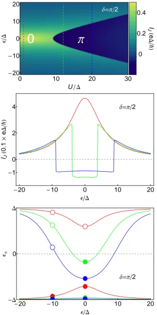
insight on this formalism. Next in subsection 3.1.2, we explain how to ex-tract from QD’s GF a first observable: the QD’s density of states. Then we analyze the GF’s expression for an asymmetric QD in section 3.1.3, and we extend our model to a double QD in which two QDs are connected in series between two superconducting electrodes in section 3.1.4. In section 3.1.5, we explain how to calculate, from QD’s GFs a second observable: the super-current flowing through the QD. We also discuss how the phenomenological model describes the singlet-doublet transition of the device and the resulting reversal of supercurrent (the so-called 0− π transition) [3, 48].
In section 3.2, we briefly introduced the NRG technique. We will discuss how one can used NRG calculations to obtain exact numerical results on the proximity effect in QD.
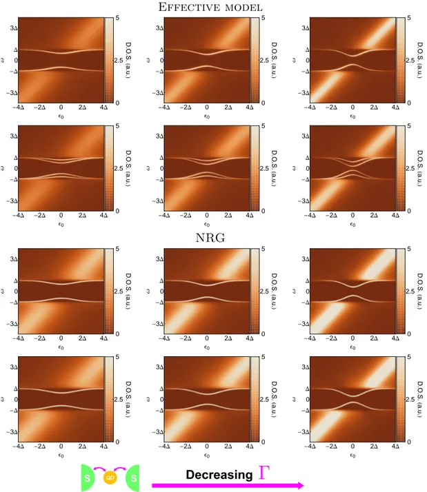
Finally in section 3.3, we analyze the influence of the physical ingre-dients of the model on the QD’s DOS and particularly on the ABSs. In parallel to this analysis, we carry out a comparison between NRG and the simplified non-interacting treatment in order to understand the limits of the phenomenological approach.
3.1
Effective description of the S-QD-S
junc-tion
3.1.1
Green’s function of a QD connected to
supercon-ducting leads
We use here exactly the same effective non-interacting picture of a QD cou-pled to superconducting leads (see section A.4.1 appendix A) as in the scat-tering description of section 2.3. However, in contrast with the scatscat-tering approach where we used known results without making explicit the Hamil-tonian of the system, here we write down this HamilHamil-tonian, as we will need it to express the GF.
3.1.1.1 Effective Hamiltonian of a S-QD-S junction
As in section 2.3, we restrict to a single orbital of the QD, as most of the relevant physics is captured in this simple case. There are at most two electrons in the dot, which then are necessarily of opposite spin, due to the Pauli principle. We also adopt the same approximate treatment of the Coulomb interaction by introducing a phenomenological breaking of the spin