HAL Id: hal-00164772
https://hal.archives-ouvertes.fr/hal-00164772
Submitted on 25 Sep 2007HAL is a multi-disciplinary open access
archive for the deposit and dissemination of sci-entific research documents, whether they are pub-lished or not. The documents may come from
L’archive ouverte pluridisciplinaire HAL, est destinée au dépôt et à la diffusion de documents scientifiques de niveau recherche, publiés ou non, émanant des établissements d’enseignement et de
Fitness landscape of the cellular automata majority
problem: View from the Olympus
Sébastien Verel, Philippe Collard, Marco Tomassini, Leonardo Vanneschi
To cite this version:
Sébastien Verel, Philippe Collard, Marco Tomassini, Leonardo Vanneschi. Fitness landscape of the cellular automata majority problem: View from the Olympus. Theoretical Computer Science, Elsevier, 2007, 378 (1), pp.54-77. �10.1016/j.tcs.2007.01.001�. �hal-00164772�
hal-00164772, version 1 - 25 Sep 2007
Fitness Landscape of the Cellular Automata
Majority Problem:
View from the ”Olympus”
S. Verel
a, P. Collard
a, M. Tomassini
band L. Vanneschi
caLaboratoire I3S, CNRS-University of Nice Sophia Antipolis, France bInformation Systems Department, University of Lausanne, Switzerland cDipartimento di Informatica Sistemistica e Comunicazione, University of
Milano-Bicocca, Italy
Abstract
In this paper we study cellular automata (CAs) that perform the computational Majority task. This task is a good example of what the phenomenon of emergence in complex systems is. We take an interest in the reasons that make this particular fitness landscape a difficult one. The first goal is to study landscape as such, and thus it is ideally independent from the actual heuristics used to search the space. However, a second goal is to understand the features a good search technique for this particular problem space should possess. We statistically quantify in various ways the degree of difficulty of searching this landscape. Due to neutrality, investigations based on sampling techniques on the whole landscape are difficult to conduct. So, we go exploring the landscape from the top. Although it has been proved that no CA can perform the task perfectly, several efficient CAs for this task have been found. Exploiting similarities between these CAs and symmetries in the landscape, we define the Olympus landscape which is regarded as the ”heavenly home” of the best local optima known (blok). Then we measure several properties of this subspace. Although it is easier to find relevant CAs in this subspace than in the overall landscape, there are structural reasons that prevents a searcher from finding overfitted CAs in the Olympus. Finally, we study dynamics and performances of genetic algorithms on the Olympus in order to confirm our analysis and to find efficient CAs for the Majority problem with low computational cost.
Key words: Fitness landscapes, Correlation analysis, Neutrality, Cellular automata, AR models
1 Introduction
Cellular automata (CAs) are discrete dynamical systems that have been stud-ied theoretically for years due to their architectural simplicity and the wide spectrum of behaviors they are capable of [1,2]. CAs are capable of universal computation and their time evolution can be complex. But many CAs show simpler dynamical behaviors such as fixed points and cyclic attractors. Here we study CAs that can be said to perform a simple “computational” task. One such tasks is the so-called majority or density task in which a two-state CA is to decide whether the initial state contains more zeros than ones or vice versa. In spite of the apparent simplicity of the task, it is difficult for a local system as a CA as it requires a coordination among the cells. As such, it is a perfect paradigm of the phenomenon of emergence in complex systems. That is, the task solution is an emergent global property of a system of locally interacting agents. Indeed, it has been proved that no CA can perform the task perfectly i.e., for any possible initial binary configuration of states [3]. However, several efficient CAs for the density task have been found either by hand or by us-ing heuristic methods, especially evolutionary computation [4,5,6,7,8,9]. For a recent review of the work done on the problem in the last ten years see [10].
All previous investigations have empirically shown that finding good CAs for the majority task is very hard. In other words, the space of automata that are feasible solutions to the task is a difficult one to search. However, there have been no investigations, to our knowledge, of the reasons that make this particular fitness landscape a difficult one. In this paper we try to statistically quantify in various ways the degree of difficulty of searching the majority CA landscape. Our investigation is a study of the fitness landscape as such, and thus it is ideally independent from the actual heuristics used to search the space provided that they use independent bit mutation as a search operator. However, a second goal of this study is to understand the features a good search technique for this particular problem space should possess.
The present study follows in the line of previous work by Hordijk [11] for another interesting collective CA problem: the synchronization task [12].
The paper proceeds as follows. The next section summarizes definitions and facts about CAs and the density task, including previous results obtained in building CAs for the task. A description of fitness landscapes and their sta-tistical analysis follows. This is followed by a detailed analysis of the majority problem fitness landscape. Next we identify and analyze a particular subspace of the problem search space called the Olympus. Finally, we present our con-clusions and hints to further works and open questions.
2 Cellular Automata and the Majority Problem
2.1 Cellular Automata
CAs are dynamical systems in which space and time are discrete. A standard CA consists of an array of cells, each of which can be in one of a finite number of possible states, updated synchronously in discrete time steps, according to a local, identical transition rule. Here we will only consider boolean automata
for which the cellular state s ∈ {0, 1}. The regular cellular array (grid) is
d-dimensional, where d = 1, 2, 3 is used in practice. For one-dimensional grids, a cell is connected to r local neighbors (cells) on either side where r is referred to as the radius (thus, each cell has 2r + 1 neighbors, including itself). The transition rule contained in each cell is specified in the form of a rule table, with an entry for every possible neighborhood configuration of states. The state of a cell at the next time step is determined by the current states of a surrounding neighborhood of cells. Thus, for a linear CA of radius r with
1≤ r ≤ N, the update rule can be written as:
sit+1 = φ(si−rt ..., s
i
t, ...si+rt ),
where st
i denotes the state of site i at time t, φ represents the local transition
rule, and r is the CA radius.
The term configuration refers to an assignment of ones and zeros to all the
cells at a given time step. It can be described by st= (s0t, s1t, . . . , sN −1t ), where
N is the lattice size. The CAs used here are linear with periodic boundary
conditions sNt +i= sit i.e., they are topologically rings.
A global update rule Φ can be defined which applies in parallel to all the cells:
st+1 = Φ(st).
The global map Φ thus defines the time evolution of the whole CA.
To visualize the behavior of a CA one can use a two-dimensional space-time
diagram, where the horizontal axis depicts the configuration st at a certain
time t and the vertical axis depicts successive time steps, with time increasing down the page (for example, see figure 1).
2.2 The Majority Problem
The density task is a prototypical distributed computational problem for CAs.
For a finite CA of size N it is defined as follows. Let ρ0 be the fraction of 1s
in the initial configuration (IC) s0. The task is to determine whether ρ0 is
(a) (b)
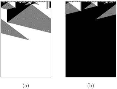
Fig. 1. Space-time diagram for the GKL rule. The density of zeros ρ0 is 0.476 in
(a) and ρ0 = 0.536 in (b). State 0 is depicted in white; 1 in black.
the majority problem. If ρ0 > 1/2 then the CA must relax to a fixed-point
configuration of all 1’s that we indicate as (1)N; otherwise it must relax to a
fixed-point configuration of all 0’s, noted (0)N, after a number of time steps
of the order of the grid size N. Here N is set to 149, the value that has been customarily used in research on the density task (if N is odd one avoids the
case ρ0 = 0.5 for which the problem is undefined).
This computation is trivial for a computer having a central control. Indeed, just scanning the array and adding up the number of, say, 1 bits will provide the answer in O(N) time. However, it is nontrivial for a small radius one-dimensional CA since such a CA can only transfer information at finite speed relying on local information exclusively, while density is a global property of the configuration of states [4].
It has been shown that the density task cannot be solved perfectly by a uni-form, two-state CA with finite radius [3], although a slightly modified version of the task can be shown to admit perfect solution by such an automaton [13]. It can also be solved perfectly by a combination of automata [14].
2.3 Previous Results on the Majority task
The lack of a perfect solution does not prevent one from searching for im-perfect solutions of as good a quality as possible. In general, given a desired global behavior for a CA (e.g., the density task capability), it is extremely difficult to infer the local CA rule that will give rise to the emergence of the computation sought. This is because of the possible nonlinearities and large-scale collective effects that cannot in general be predicted from the sole local CA updating rule, even if it is deterministic. Since exhaustive evaluation of all
possible rules is out of the question except for elementary (d = 1, r = 1) and perhaps radius-two automata, one possible solution of the problem consists in using evolutionary algorithms, as first proposed by Packard in [15] and further developed by Mitchell et al. in [5,4].
The performance of the best rules found at the end of the evolution is eval-uated on a larger sample of ICs and it is defined as the fraction of correct
classifications over n = 104 randomly chosen ICs. The ICs are sampled
ac-cording to a binomial distribution (i.e., each bit is independently drawn with probability 1/2 of being 0).
Mitchell and coworkers performed a number of studies on the emergence of synchronous CA strategies for the density task (with N = 149) during evo-lution [5,4]. Their results are significant since they represent one of the few instances where the dynamics of emergent computation in complex, spatially extended systems can be understood. In summary, these findings can be sub-divided into those pertaining to the evolutionary history and those that are part of the “final” evolved automata. For the former, they essentially observed that, in successful evolution experiments, the fitness of the best rules increases in time according to rapid jumps, giving rise to what they call “epochs” in the evolutionary process. Each epoch corresponds roughly to a new, increasingly sophisticated solution strategy. Concerning the final CA produced by evolu-tion, it was noted that, in most runs, the GA found unsophisticated strategies that consisted in expanding sufficiently large blocks of adjacent 1s or 0s. This “block-expanding” strategy is unsophisticated in that it mainly uses local in-formation to reach a conclusion. As a consequence, only those IC that have low or high density are classified correctly since they are more likely to have extended blocks of 1s or 0s. In fact, these CA have a performance around 0.6. However, some of the runs gave solutions that presented novel, more so-phisticated features that yielded better performance (around 0.77) on a wide distribution of ICs. However, high-performance automata have evolved only nine times out of 300 runs of the genetic algorithm. This clearly shows that it is very difficult for genetic algorithm to find good solutions in this the search space.
These new strategies rely on traveling signals that transfer spatial and tem-poral information about the density in local regions through the lattice. An example of such a strategy is given in Figure 1, where the behavior of the so-called GKL rule is depicted [4]. The GKL rule is hand-coded but its behavior is similar to that of the best solutions found by evolution. Crutchfield and coworkers have developed sophisticated methodologies for studying the trans-fer of long-range signals and the emergence of computation in evolved CA. This framework is known as “computational mechanics” and it describes the intrinsic CA computation in terms of regular domains, particles, and particle interactions. Details can be found in [16,17,10].
Andre et al. in [7] have been able to artificially evolve a better CA by using genetic programming. Finally, Juill´e and Pollack [8] obtained still better CAs by using a coevolutionary algorithm. Their coevolved CA has performance
about 0.86, which is the best result known to date.
3 Fitness Landscapes
3.1 Introduction
First we recall a few fundamental concepts about fitness landscapes (see [18,19] for a more detailed treatment). A landscape is a triplet (S, f, N) where S is
a set of potential solutions (also called search space), N : S → 2S, a
neigh-borhood structure, is a function that assigns to every s∈ S a set of neighbors
N(s), and f : S 7→ IR is a fitness function that can be pictured as the “height”
of the corresponding potential solutions.
Often a topological concept of distance d can be associated to a neighborhood
N. A distance d : S × S 7→ IR+ is a function that associates with any two
configurations in S a nonnegative real number that verifies well-known prop-erties.
For example, for a binary coded GA, the fitness landscape S is constituted by
the boolean hypercube B = {0, 1}l consisting of the 2l solutions for strings
of length l and the associated fitness values. The neighborhood of a solution,
for the one-bit random mutation operator, is the set of points y∈ B that are
reachable from x by flipping one bit. A natural definition of distance for this landscape is the well-known Hamming distance.
Based on the neighborhood notion, one can define local optima as being
con-figurations x for which (in the case of maximization): ∀y ∈ N(x), f(y) ≤ f(x)
Global optima are defined as being the absolute maxima (or minima) in the whole of S. Other features of a landscape such as basins, barriers, or neutrality can be defined likewise[18]. Neutrality is a particularly important notion in our study, and will be dealt with further.
A notion that will be used in the rest of this work is that of a walk on a
landscape. A walk Γ from s to s′
is a sequence Γ = (s0, s1, . . . , sm) of solutions
belonging to S where s0 = s, sm = s
′
and ∀i ∈ [1, m], si is a neighbor of si−1.
The walk can be random, for instance solutions can be chosen with uniform probability from the neighborhood, as in random sampling, or according to other weighted non-uniform distributions, as in Monte Carlo sampling, for example. It can also be obtained through the repeated application of a “move” operator, either stochastic or deterministic, defined on the landscape, such as a form of mutation or a deterministic hill-climbing strategy.
3.2 Neutrality
The notion of neutrality has been suggested by Kimura [20] in his study of the evolution of molecular species. According to this view, most mutations are neutral (their effect on fitness is small) or lethal.
In the analysis of fitness landscapes, the notion of neutral mutation appears to be useful [21]. Let us thus define more precisely the notion of neutrality for fitness landscapes.
Definition: A test of neutrality is a predicate isNeutral : S × S → {true,
f alse} that assigns to every (s1, s2) ∈ S2 the value true if there is a small
difference between f (s1) and f (s2).
For example, usually isNeutral(s1, s2) is true if f (s1) = f (s2). In that case,
isNeutral is an equivalence relation. Other useful cases are isNeutral(s1, s2)
is true if |f(s1)− f(s2)| ≤ 1/M with M is the population size. When f is
stochastic, isNeutral(s1, s2) is true if |f(s1)− f(s2)| is under the evaluation
error.
Definition:For every s∈ S, the neutral neighborhood of s is the set Nneut(s) =
{s′
∈ N(s) | isNeutral(s, s′
)} and the neutral degree of s, noted nDeg(s) is
the number of neutral neighbors of s, nDeg(s) = ♯(Nneut(s)− {s}).
A fitness landscape is neutral if there are many solutions with high neutral degree. In this case, we can imagine fitness landscapes with some plateaus called neutral networks. Informally, there is no significant difference of fitness between solutions on neutral networks and the population drifts around on them.
Definition: A neutral walk Wneut = (s0, s1, . . . , sm) from s to s
′
is a walk
from s to s′
where for all (i, j)∈ [0, m]2 , isNeutral(s
i, sj) is true.
Definition: A Neutral Network, denoted NN, is a graph G = (V, E) where
the set V of vertices is the set of solutions belonging to S such that for all s
and s′ from V there is a neutral walk Wneut belonging to V from s to s
′ , and two vertices are connected by an edge of E if they are neutral neighbors.
Definition: A portal in a NN is a solution which has at least one neighbor
3.3 Statistical Measures on Landscapes
3.3.1 Density of States
H. Ros´e et al. [22] develop the density of states approach (DOS) by plotting the number of sampled solutions in the search space with the same fitness value. Knowledge of this density allows to evaluate the performance of random search or random initialization of metaheuristics. DOS gives the probability of having a given fitness value when a solution is randomly chosen. The tail of the distribution at optimal fitness value gives a measure of the difficulty of an optimization problem: the faster the decay, the harder the problem.
3.3.2 Neutrality
To study the neutrality of fitness landscapes, we should be able to measure and describe a few properties of NN. The following quantities are useful. The size ♯NN i.e., the number of vertices in a NN, the diameter, which is the
longest distance over the distance1 between two solutions belonging to NN.
The neutral degree distribution of solutions is the degree distribution of the vertices in a NN. Together with the size and the diameter, it gives informa-tion which plays a role in the dynamics of metaheuristic [23,24]. Huynen [25] defined the innovation rate of NN to explain the advantage of neutrality in fitness landscapes. This rate is the number of new, previously unencountered fitness values observed in the neighborhood of solutions along a neutral walk on NN. Finally, NN percolate the landscape if they come arbitrarily close to almost any every other NN ; this means that, if the innovation rate is high, a neutral path could be a good way to explore the landscape.
Another way to describe NN is given by the autocorrelation of neutral degree along a neutral random walk [26]. From neutral degree collected along this neutral walk, we computed its autocorrelation (see section 3.3.4). The auto-correlation measures the auto-correlation structure of a NN. If the auto-correlation is low, the variation of neutral degree is low ; and so, there is some areas in NN of solutions which have nearby neutral degrees.
3.3.3 Fitness Distance Correlation
This statistic was first proposed by Jones [19] with the aim of measuring the difficulty of problems with a single number. Jones’s approach states that what makes a problem hard is the relationship between fitness and distance of the solutions from the optimum. This relationship can be summarized by
calculating the fitness-distance correlation coefficient (FDC). Given a set F =
{f1, f2, ..., fm} of m individual fitness values and a corresponding set D =
{d1, d2, ..., dm} of the m distances to the nearest global optimum, FDC is
defined as: F DC = CF D σFσD where: CF D = 1 m m X i=1 (fi− f)(di− d)
is the covariance of F and D and σF, σD, f and d are the standard deviations
and means of F and D. Thus, by definition, FDC ∈ [−1, 1]. As we hope that
fitness increases as distance to a global optimum decreases (for maximization problems), we expect that, with an ideal fitness function, FDC will assume
the value of −1. According to Jones [19], GA problems can be classified in
three classes, depending on the value of the FDC coefficient:
• Misleading (F DC ≥ 0.15), in which fitness increases with distance.
• Difficult (−0.15 < F DC < 0.15) in which there is virtually no correlation between fitness and distance.
• Straightforward (F DC ≤ −0.15) in which fitness increases as the global optimum approaches.
The second class corresponds to problems for which the FDC coefficient does
not bring any information. The threshold interval [−0.15, 0.15] has been
em-pirically determined by Jones. When FDC does not give a clear indication
i.e., in the interval [−0.15, 0.15], examining the scatterplot of fitness versus
distance can be useful.
The FDC has been criticized on the grounds that counterexamples can be constructed for which the measure gives wrong results [27,28,29]. Another drawback of FDC is the fact that it is not a predictive measure since it re-quires knowledge of the optima. Despite its shortcomings, we use FDC here as another way of characterizing problem difficulty because we know some optima and we predict whether or not it is easy to reach those local optima.
3.3.4 The Autocorrelation Function and the Box-Jenkins approach
Weinberger [30,31] introduced the autocorrelation function and the corre-lation length of random walks to measure the correcorre-lation structure of
fit-ness landscapes. Given a random walk (st, st+1, . . .), the autocorrelation
func-tion ρ of a fitness funcfunc-tion f is the autocorrelafunc-tion funcfunc-tion of time series
(f (st), f (st+1), . . .) :
ρ(k) = E[f (st)f (st+k)]− E[f(st)]E[f (st+k)]
where E[f (st)] and var(f (st)) are the expected value and the variance of
f (st). Estimates r(k) of autocorrelation coefficients ρ(k) can be calculated
with a time series (s1, s2, . . . , sL) of length L :
r(k) = PL−k j=1(f (sj)− ¯f )(f (sj+k)− ¯f ) PL j=1(f (sj)− ¯f )2 where ¯f = 1 L PL
j=1f (sj), and L >> 0. A random walk is representative of
the entire landscape when the landscape is statistically isotropic. In this case, whatever the starting point of random walks and the selected neighbors dur-ing the walks, estimates of r(n) must be nearly the same. Estimation error diminishes with the walk length.
The correlation length τ measures how the autocorrelation function decreases and it summarizes the ruggedness of the landscape: the larger the correlation
length, the smoother is the landscape. Weinberger’s definition τ = − 1
ln(ρ(1))
makes the assumption that the autocorrelation function decreases exponen-tially. Here we will use another definition that comes from a more general analysis of time series, the Box-Jenkins approach [32], introduced in the field of fitness landscapes by Hordijk [33]. The time series of fitness values will be ap-proached by an autoregressive moving-average (ARMA) model. In ARMA(p, q) model, the current value depends linearly on the p previous values and the q previous white noises.
f (st) = c + p X i=1 αif (st−i) + ǫt+ q X i=1
βiǫt−i where ǫt are white noises.
The approach consists in the iteration of three stages [32]. The identification stage consists in determining the value of p and q using the autocorrelation function (acf) and the partial autocorrelation function (pacf) of the time series.
The estimation stage consists in determining the values c, αi and βi using the
pacf. The significance of this values is tested by a t-test. The value is not significant if t-test is below 2. The diagnostic checking stage is composed of two parts. The first one checks the adequation between data and estimated
data. We use the square correlation R2 between observed data of the time
series and estimated data produced by the model and the Akaide information criterion AIC:
AIC(p, q) = log(ˆσ2) + 2(p + q)/L where ˆσ2 = L−1
L
X
j=1
(yj− ˆyj)2
The second one checks the white noise of residuals which is the difference be-tween observed data value and estimated values. For this, the autocorrelation of residuals and the p-value of Ljung-Box test are computed.
3.4 Fitness Cloud and NSC
We use the fitness cloud (FC) standpoint, first introduced in [34] by V´erel and coworkers. The fitness cloud relative to the local search operator op is
the conditional bivariate probability density Pop(Y = ˜ϕ | X = ϕ) of reaching
a solution of fitness value ˜ϕ from a solution of fitness value ϕ applying the
operator op. To visualize the fitness cloud in two dimensions, we plot the
scatterplot F C ={(ϕ, ˜ϕ) | Pop(ϕ, ˜ϕ)6= 0}.
In general, the size of the search space does not allow to consider all the possible individuals, when trying to draw a fitness cloud. Thus, we need to use samples to estimate it. We prefer to sample the space according to a distribution that gives more weight to “important” values in the space, for instance those at a higher fitness level. This is also the case of any biased searcher such as an evolutionary algorithm, simulated annealing and other heuristics, and thus this kind of sampling process more closely simulates the way in which the program space would be traversed by a searcher. So, we use the Metropolis-Hastings technique [35] to sample the search space.
The Metropolis-Hastings sampling technique is an extension of the Metropolis algorithm to non-symmetric stationary probability distributions. It can be defined as follows. Let α be the function defined as:
α(x, y) = min{1,y
x},
and f (γk) be the fitness of individual γk. A sample of individuals{γ1, γ2, . . . , γn}
is built with the algorithm shown in figure 2.
In order to algebraically extract some information from the fitness cloud, in [36,37], we have defined a measure, called negative slope coefficient (nsc). The
abscissas of a scatterplot can be partitioned into m segments {I1, I2, . . . , Im}
with various techniques. Analogously, a partition of the ordinates {J1, J2, . . . ,
Jm} can be done, where each segment Ji contains all the ordinates
corre-sponding to the abscissas contained in Ii. Let M1, M2, . . . , Mm be the
aver-ages of the abscissa values contained inside the segments I1, I2, . . . , Im and let
N1, N2, . . . , Nm be the averages of the ordinate values in J1, J2, . . . , Jm. Then
we can define the set of segments {S1, S2, . . . , Sm−1}, where each Si connects
the point (Mi, Ni) to the point (Mi+1, Ni+1). For each one of these segments
Si, the slope Pi can be calculated as follows:
Pi =
Ni+1− Ni
begin
γ1 is generated uniformly at random;
for k:= 2 to n do
1. an individual δ is generated uniformly at random; 2. a random number u is generated from a
uniform (0, 1) distribution; 3. if (u≤ α(f(γk−1), f (δ))) then γk := δ else goto 1. endif 4. k:= k + 1; endfor end
Fig. 2. The algorithm for sampling a search space with the Metropolis-Hastings technique.
Finally, we can define the NSC as: nsc =
m−1X i=1
ci, where: ∀i ∈ [1, m) ci = min(Pi, 0)
We hypothesize that nsc can give some indication of problem difficulty in the following sense: if nsc= 0, the problem is easy, if nsc< 0 the problem is difficult and the value of nsc quantifies this difficulty: the smaller its value, the more difficult the problem. In other words, according to our hypothesis, a problem
is difficult if at least one of the segments S1, S2, . . . , Sm−1 has a negative slope
and the sum of all the negative slopes gives a measure of problem hardness. The idea is that the presence of a segment with negative slope indicates a bad evolvability for individuals having fitness values contained in that segment.
4 Analysis of the Majority Problem Fitness Landscape
4.1 Definition of the fitness landscape
As in Mitchell [4], we use CA of radius r = 3 and configurations of length N = 149. The set S of potential solutions of the Majority Fitness Landscape is the set of binary string which represent the possible CA rules. The size of
S is 222r+1
= 2128, and each automaton should be tested on the 2149 possible
different ICs. This gives 2277 possibilities, a size far too large to be searched
ex-haustively. Since performance can be defined in several ways, the consequence is that for each feasible CA in the search space, the associated fitness can be
different, and thus effectively inducing different landscapes. In this work we will use one type of performance measure based on the fraction of n initial configurations that are correctly classified from one sample. We call standard performance (see also section 2.3) the performance when the sample is drawn from a binomial distribution (i.e., each bit is independently drawn with prob-ability 1/2 of being 0). Standard performance is a hard measure because of the predominance in the sample of ICs close to 0.5 and it has been typically employed to measure a CA’s capability on the density task.
The standard performance cannot be known perfectly due to random varia-tion of samples of ICs. The fitness funcvaria-tion of the landscape is stochatic one which allows population of solutions to drift arround neutral networks. The error of evaluation leads us to define the neutrality of landscape. The ICs are chosen independently, so the fitness value f of a solution follows a normal law
N (f,σ(f )√n), where σ is the standard deviation of sample of fitness f , and n is the
sample size. For binomial sample, σ2(f ) = f (1− f), the variance of Bernouilli
trial. Then two neighbors s and s′ are neutral neighbors (isNeutral(s, s′) is
true) if a t-test accepts the hypothesis of equality of f (s) and f (s′
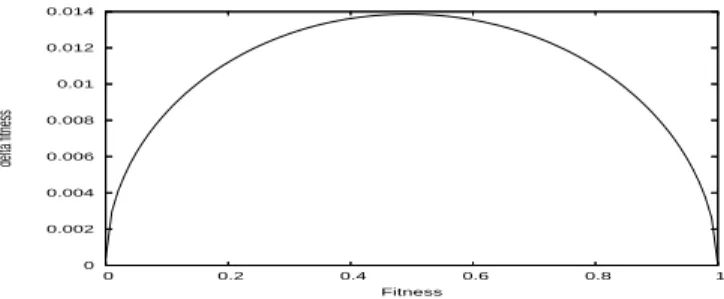
) with 95 percent of confidence (fig. 3). The maximum number of fitness values
statis-tically different for standard performance is 113 for n = 104, 36 for n = 103
and 12 for n = 102. 0 0.002 0.004 0.006 0.008 0.01 0.012 0.014 0 0.2 0.4 0.6 0.8 1 delta fitness Fitness
Fig. 3. Error of standard performance as a function of standard performance given by t-test with 95 percent of confidence with sample of size n = 104. Bitflip is neutral if the absolute value of the difference between the two fitnesses is above the curve.
4.2 First statistical Measures
The DOS of the Majority problem landscape was computed using the uni-form random sampling technique. The number of sampled points is 4000 and, among them, the number of solutions with a fitness value equal to 0 is 3979. Clearly, the space appears to be a difficult one to search since the tail of the distribution to the right is non-existent. Figure 4 shows the DOS obtained using the Metropolis-Hastings technique. This time, over the 4000 solutions sampled, only 176 have a fitness equal to zero, and the DOS clearly shows a more uniform distribution of rules over many different fitness values.
0 0.05 0.1 0.15 0.2 0 0.1 0.2 0.3 0.4 0.5 0 0.01 0.02 0.03 0.04 0.05 0.06 0.45 0.46 0.47 0.48 0.49 0.5 0.51 0.52 (a) (b)
Fig. 4. DOS obtained using the Metropolis-Hastings technique to sample the search space, between fitness values 0.0 and 0.52 in (a) and between 0.45 and 0.52 in (b). x-axis: fitness values; y-axis: fitness values frequencies.
It is important to remark a considerable number of solutions sampled with a fitness approximately equal to 0.5. Furthermore, no individual with a fitness value superior to 0.514 has been sampled. For the details of the techniques used to sample the space, see [36,37]
The autocorrelation along random walks is not significant due to the large number of zero fitness points and is thus not reported here.
The FDC, calculated over a sample of 4000 individuals generated using the Metropolis-Hastings technique, are shown in table 1. Each value has been obtained using one of the best local optima known to date (see section 4.4). FDC values are approximately close to zero for DAS optimum. For ABK optimum, FDC value is near to -0.15, value identified by Jones as the threshold between difficult and straightforward problems. For all the other optima, FDC
are close to−0.10. So, the FDC does not provide information about problem
difficulty.
Table 1
FDC values for the six best optima known, calculated over a sample of 4000 solutions generated with the Metropolis-Hastings sampling technique.
Rules GLK [38] Davis [7] Das [39] ABK [7] Coe1 [40] Coe2 [40] FDC -0.1072 -0.0809 -0.0112 -0.1448 -0.1076 -0.1105
Figure 5 shows the fitness cloud, and the set of segments used to calculate the NSC. As this figure clearly shows, the Metropolis-Hastings technique allows to sample a significant number of solutions with a fitness value higher than
zero. The value of the NSC for this problem is −0.7133, indicating that it
Table 2
Description of the starting of neutral walks.
00000000 00000110 00010000 00010100 00001010 01011000 01111100 01001101
0.5004 01000011 11101101 10111111 01000111 01010001 00011111 11111101 01010111 00000101 00000100 00000101 10100111 00000101 00000000 00001111 01110111
0.7645 00000011 01110111 01010101 10000011 01111011 11111111 10110111 01111111
and going further seems to be much harder.
0.05 0.1 0.15 0.2 0.25 0.3 0.35 0.4 0.45 0.5 0.55 Fitness 0.05 0.1 0.15 0.2 0.25 0.3 0.35 0.4 0.45 0.5 0.55 Fitness 0 0.05 0.1 0.15 0.2 0.25 0.3 0.35 0.4 0 0.1 0.2 0.3 0.4 0.5 0.6 0 0.1 0.2 0.3 0.4 0.5 0.6 Fitness Fitness
Fig. 5. Fitness Cloud and Scatterplot used to calculate the NSC value. Metropo-lis-Hastings technique has been used to sample the search space.
4.3 Neutrality
Computational costs do not allow us to analyze many neutral networks. In this section we analyze two important large neutral networks (NN). A large num-ber of CAs solve the majority density problem on only half of ICs because they
converge nearly always on the final configuration (O)N or (1)N and thus have
performance about 0.5. Mitchell [5] calls these “default strategies” and notices that they are the first stage in the evolution of the population before jumping to higher performance values associated to “block-expanding” strategies (see
section 2.3). We will study this large NN, denoted NN0.5 around standard
performance 0.5 to understand the link between NN properties and GA
evo-lution. The other NN, denoted NN0.76, is the NN around fitness 0.7645 which
contains one neighbor of a CA found by Mitchell et al. The description of this “high” NN could give clues as how to “escape” from NN toward even higher fitness values.
In our experiments, we perform 5 neutral walks on NN0.5 and 19 on NN0.76.
Each neutral walk has the same starting point on each NN. The solution with performance 0.5 is randomly solution and the solution with performance
0.76 is a neighboring solution of solution find by Mitchell (see tab 2). We try to explore the NN by strictly increasing the Hamming distance from the starting solution at each step of the walk. The neutral walk stops when there is no neutral step that increases distance. The maximum length of walk is thus
128. On average, the length of neutral walks on NN0.5 is 108.2 and 33.1 on
NN0.76. The diameter (see section 3.3.2) of NN0.5 should probably be larger
than the one of NN0.76.
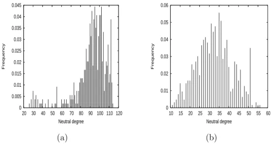
0 0.005 0.01 0.015 0.02 0.025 0.03 0.035 0.04 0.045 20 30 40 50 60 70 80 90 100 110 120 Frequency Neutral degree 0 0.01 0.02 0.03 0.04 0.05 0.06 10 15 20 25 30 35 40 45 50 55 60 Frequency Neutral degree (a) (b)
Fig. 6. Distribution of Neutral Degree along all neutral walks on N N0.5 in (a) and
N N0.76 in (b).
Figure 6 shows the distribution of neutral degree collected along all neutral
walks. The distribution is close to normal for NN0.76. For NN0.5 the
distribu-tion is skewed and approximately bimodal with a strong peak around 100 and
a small peak around 32. The average of neutral degree on NN0.5 is 91.6 and
standard deviation is 16.6; on NN0.76, the average is 32.7 and the standard
deviation is 9.2. The neutral degree for NN0.5 is very high : 71.6 % of
neigh-bors are neutral neighneigh-bors. For NN0.76, there is 25.5 % of neutral neighbors. It
can be compared to the average neutral degree overall neutral NKq-landscape with N = 64, K = 2 and q = 2 which is 33.3 % [41].
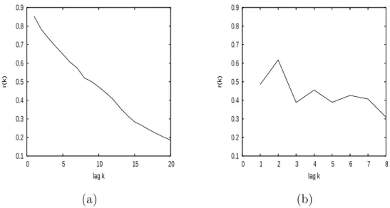
Figure 7 gives an estimation of the autocorrelation function of neutral degree of the neutral networks. The autocorrelation function is computed for each
neutral walk and the estimation r(k) of ρ(k) is given by the average of ri(k)
over all autocorrelation functions. For both NN, there is correlation. The
cor-relation is higher for NN0.5 (ρ(1) = 0.85) than for NN0.76(ρ(1) = 0.49). From
the autocorrelation of the neutral degree, one can conclude that the neutral network topology is not completely random, since otherwise correlation should have been nearly equal to zero. Moreover, the variation of neutral degree is smooth on NN; in other words, the neighbors in NN have nearby neutral degrees. So, there is some area where the neutral degree is homogeneous.
0.1 0.2 0.3 0.4 0.5 0.6 0.7 0.8 0.9 0 5 10 15 20 r(k) lag k 0.1 0.2 0.3 0.4 0.5 0.6 0.7 0.8 0.9 0 1 2 3 4 5 6 7 8 r(k) lag k (a) (b)
Fig. 7. Estimation of the autocorrelation function of neutral degrees along neutral random walks for N N0.5 (a) and for N N0.76 (b).
0 10 20 30 40 50 0 20 40 60 80 100 120
Number of new fitness values
Step Innovation rate nb advantageus innovation 0 10 20 30 40 50 0 5 10 15 20 25 30 35 40 45
Number of new fitness values
Step
Innovation rate nb advantageus innovation
(a) (b)
Fig. 8. Innovation rate along one neutral random walk. Fitness of the neutral net-works is 0.5004 (a) and 0.7645 (b).
The innovation rate and the number of new better fitnesses found along the longest neutral random walk for each NN is given in figure 8. The majority of new fitness value found along random walk is deleterious, very few solutions are fitter.
This study give us a better description of Majority fitness landscape neutral-ity which have important consequence on metaheuristic design. The neutral degree is high. Therefore, the selection operator should take into account the case of equality of fitness values. Likewise the mutation rate and population size should fit to this neutral degree in order to find rare good solutions out-side NN [42]. For two potential solutions x and y on NN, the probability
Table 3
Description and standard performance of the 6 previously known best rules (blok ) computed on sample size of 104.
GLK 00000000 01011111 00000000 01011111 00000000 01011111 00000000 01011111 0.815 00000000 01011111 11111111 01011111 00000000 01011111 11111111 01011111 Das 00000000 00101111 00000011 01011111 00000000 00011111 11001111 00011111 0.823 00000000 00101111 11111100 01011111 00000000 00011111 11111111 00011111 Davis 00000111 00000000 00000111 11111111 00001111 00000000 00001111 11111111 0.818 00001111 00000000 00000111 11111111 00001111 00110001 00001111 11111111 ABK 00000101 00000000 01010101 00000101 00000101 00000000 01010101 00000101 0.824 01010101 11111111 01010101 11111111 01010101 11111111 01010101 11111111 Coe1 00000001 00010100 00110000 11010111 00010001 00001111 00111001 01010111 0.851 00000101 10110100 11111111 00010111 11110001 00111101 11111001 01010111 Coe2 00010100 01010001 00110000 01011100 00000000 01010000 11001110 01011111 0.860 00010111 00010001 11111111 01011111 00001111 01010011 11001111 01011111
P (x6∈ NN) + P (y 6∈ NN) − P (x 6∈ NN ∩ y 6∈ NN). This probability is higher
when solutions x and y are far due to the correlation of neutral degree in NN. To maximize the probability of escaping NN the distance between potential solutions of population should be as far as possible on NN. The population of an evolutionary algorithm should spread over NN.
4.4 Study of the best local optima known
We have seen that it is difficult to have some relevant informations on the Majority Problem landscape by random sampling due to the large number of solutions with zero fitness. In this section, we will study the landscape from the top. Several authors have found fairly good solutions for the density problem, either by hand or, especially, using evolutionary algorithms [38,39,7,40]. We
will consider the six Best Local Optima Known2, that we call blok, with a
standard performance over 0.81 (tab. 3). In the following, we will see where the blok are located and what is the structure of the landscape around these optima.
Table 4
Distances between the six best local optima known
GLK Davis Das ABK Coe1 Coe2 average
GLK 0 20 62 56 39 34 28.6 Davis 20 0 58 56 45 42 33 Das 62 58 0 50 59 44 35.4 ABK 56 56 50 0 51 54 36.6 Coe1 39 45 59 51 0 51 43 Coe2 34 42 44 54 51 0 39 4.4.1 Spatial Distribution
In this section, we study the spatial distribution of the six blok. Table 4 gives the Hamming distance between these local optima. All the distances are lower than 64 which is the distance between two random solutions. Local optima do not seem to be randomly distributed over the landscape. Some are nearby, for instance GLK and Davis rules, or GLK and Coe2 rules. But Das and GLK rules, or Coe1 and Das rules are far away from each other.
Figure 9 represents the centroid (C) of the blok. The ordinate is the frequency of appearance of bit value 1 at each bit. On the right column we give the number of bits which have the same given frequency. For six random solutions in the fitness landscape, on average the centroid is the string with 0.5 on the 128 bits and the number of bits with the same frequency of 1 follows the binomial law 2, 12, 30, 40, 30, 12, 2. On the other hand, for the six best local optima, a large number of bits have the same value (29 instead of 4 in the random case) and a smaller number of bits (22 instead of 40 in the random case) are “undecided” with a frequency of 0.5.
The local optima from the blok are not randomly distributed over the land-scape. They are all in a particular hyperspace of dimension 29 defined by the following schema S:
000*0*** 0******* 0***0*** *****1** 000***** 0*0***** ******** *****1*1 0*0***** ******** *****1** ***1*111 ******** ***1***1 *******1 ***1*111
We can thus suppose that the fixed bits are useful to obtain good solutions. Thus, the research of a good rule would be certainly more efficient in the subspace defined by schemata S. Before examining this conjecture, we are going to look at the landscape “from the top”.
1 5/6 2/3 1/2 1/3 1/6 0 0 20 40 60 80 100 120 15 15 23 22 23 16 14 frequence of 1 number of apparition number of gene
Fig. 9. Centroid C of the six blok. The squares give the frequency of 1 over the six blok as function of bits position. The right column gives the number of bits of C from the 128 which have the same frequency of 1 indicated by the ordinate in the ordinate (left column).
4.4.2 Evolvability horizon
Altenberg defined evolvability as the ability to produce fitter variants [43]. The idea is to analyze the variation in fitness between one solution and its neighbors. Evolvability is said positive if neighbor solutions are fitter than the solution and negative otherwise. In this section, we define the evolvability horizon (EH) as the sequence of solutions, ordered by fitness values, which can be reached with one bitflip from the given solution. We obtain a graph with fitness values in ordinates and the corresponding neighbors in abscissa sorted by fitnesses (see figure 10).
Figure 10 shows the evolvability horizon of the blok. There is no neighbor with a better fitness value than the initial rule; so, all the best known rules are local optima. The fitness landscape has two important neutral networks at fitness
0 (NN0) and fitness 0.5 (NN0.5) (see section 4.3). No local optimum is nearby
NN0; but a large part of neighbors of local optima (around 25% on average)
are in NN0.5. As a consequence a neutral local search on NN0.5can potentially
find a portal toward the blok.
For each EH, there is an abscissa r from which the fitness value is roughly
linear. Let fr be this fitness value, f128 the fitness of the less sensible bit, and
m the slope of the curve between abscissa r and 128. Thus, the smaller m and r, the better the neighbors. On the contrary, higher slope and r values mean that the neighbor fitness values decay faster.
For example evolvability is slightly negative from GLK, as it has a low slope and a small r. At the opposite, the Coe2 rule has a high slope ; this optimum is thus isolated and evolvability is strongly negative. We can imagine the space ”view from GLK” flatter than the one from Coe2.
Although all EH seem to have roughly the same shape (see fig. 10), we can ask whether flipping one particular bit changes the fitness in the same way. For instance, for all the optima, flipping the first bit from ’0’ to ’1’ causes a drop in fitness. More generally, flipping each bit, we compute the average and standard deviation of the difference in fitnesses; results are sorted into increasing average differences (see figure 13-a). The bits which are the more deleterious are the ones with the smaller standard deviation, and as often as not, are in the schemata S. So, the common bits in the blok seem to be important to find good solution: for a metaheuristic, it would be of benefit to search in the subspace defined by the schema S.
0.9 0.8 0.7 0.6 0.5 0.4 fr r fitness genes 0.8178 0.9 0.8 0.7 0.6 0.5 0.4 fr r fitness genes 0.8216 GLK: r = 53, m = 0.000476 Das: r = 69, m = 0.00106 0.9 0.8 0.7 0.6 0.5 0.4 fr r fitness genes 0.8147 0.9 0.8 0.7 0.6 0.5 0.4 fr r fitness genes 0.8231 Davis: r = 62, m = 0.000871 ABK: r = 41, m = 0.00114 0.9 0.8 0.7 0.6 0.5 0.4 fr r fitness genes 0.8578 0.9 0.8 0.7 0.6 0.5 0.4 fr r fitness genes 0.8578 Coe1: r = 68, m = 0.00170 Coe2: r = 62, m = 0.00424
Fig. 10. Evolvability horizon for the 6 best known rules computed on binomial sample of ICs of size 104. For each rule, the dotted horizontal line is its fitness. Row
5 Olympus Landscape
We have seen that there are many similarity inside the blok. In this section we will use this feature to define the Olympus Landscape and, to show and exploit, the relevant properties of this subspace.
5.1 Definition
The Olympus Landscape is a subspace of the Majority problem landscape. It takes its name from the Mount Olympus which is traditionally regarded as the heavenly home of the ancient Greek gods. Before defining this subspace we study the two natural symmetries of the majority problem.
The states 0 and 1 play the same role in the computational task ; so flipping bits in the entry of a rule and in the result have no effect on performance. In the same way, CAs can compute the majority problem according to right or left
direction without changing performance. We denote S01 and Srl respectively
the corresponding operator of 0/1 symmetry and right/lef t symmetry. Let
x = (x0, . . . , xλ−1)∈ {0, 1}λ be a solution with λ = 22r+1. The 0/1 symmetric
of x is S01(x) = y where for all i, yi = 1− xλ−i. The right/lef t symmetric of
x is Srl(x) = y where for all i, yi = xσ(i) with σ(Pλ−1j=0 2nj) =
Pλ−1
j=02λ−1−nj.
The operators are commutative: SrlS01 = S01Srl. From the 128 bits, 16 are
invariant by Srl symmetry and none by S01. Symmetry allows to introduce
diversity without losing quality ; so evolutionary algorithm could be improved
using the operators S01 and Srl.
We have seen that some bit values could be useful to reach a good solution (see subsection 4.4.2), and some of those are among the 29 joint bits of the blok (see subsection 4.4.1). Nevertheless, two optima from the blok could be distant whereas some of theirs symmetrics are closer. Here the idea is to choose for each blok one symmetric in order to broadly maximize the number of joint bits. The optima GLK, Das, Davis and ABK have only 2 symmetrics because
symmetrics by S01 and Srl are equal. The optima Coe1 and Coe2 have 4
sym-metrics. So, there are 24.42 = 256 possible sets of symmetrics. Among these
sets, we establish the maximum number of joint bits which is possible to obtain is 51. This “optimal” set contains the six Symmetrics of Best Local Optima
Known (blok′
) presented in table 5. The Olympus Landscape is defined from
the blok′ as the schemata S′ with the 51 fixed bits above:
000*0*0* 0****1** 0***00** **0**1** 000***** 0*0**1** ******** 0*0**1*1 0*0***** *****1** 111111** **0**111 ******** 0**1*1*1 11111**1 0*01*111
Table 5
Description of the 6 symmetrics of the best local optima known (blok′) chosen to maximize the number of joint bits.
GLK′ 00000000 01011111 00000000 01011111 00000000 01011111 00000000 01011111 = GLK 00000000 01011111 11111111 01011111 00000000 01011111 11111111 01011111 Das′ 00000000 00101111 00000011 01011111 00000000 00011111 11001111 00011111 = Das 00000000 00101111 11111100 01011111 00000000 00011111 11111111 00011111 Davis′ 00000000 00001111 01110011 00001111 00000000 00011111 11111111 00001111 = S01(Davis) 00000000 00001111 11111111 00001111 00000000 00011111 11111111 00011111 ABK′ 00000000 01010101 00000000 01010101 00000000 01010101 00000000 01010101 = S01(ABK) 01011111 01010101 11111111 01011111 01011111 01010101 11111111 01011111 Coe1′ 00000001 00010100 00110000 11010111 00010001 00001111 00111001 01010111 = Coe1 00000101 10110100 11111111 00010111 11110001 00111101 11111001 01010111 Coe2′ 00010100 01010101 00000000 11001100 00001111 00010100 00000010 00011111 = Srl(Coe2) 00010111 00010101 11111111 11001111 00001111 00010111 11111111 00011111 Table 6
Distances between the symmetrics of the Best Local Optima Known (blok′) GLK′ Davis′ Das′ ABK′ Coe1′ Coe2′ average
GLK′ 0 20 26 24 39 34 23.8 Davis′ 20 0 14 44 45 42 27.5 Das′ 26 14 0 50 43 44 29.5 ABK′ 24 44 50 0 39 26 30.5 Coe1′ 39 45 43 39 0 49 35.8 Coe2′ 34 42 44 26 49 0 32.5
The Olympus Landscape is a subspace of dimension 77. All the fixed bits from
schema S (see section 4.4.1) are fixed in the schema S′
with the same value except for the bit number 92.
Table 6 gives the Hamming distance between the six blok′
. All the distances are shorter than those between the blok (see table 4). On average, distance
between the rules is 29.93 for the blok′ and 35.93 for the blok. Rules in the
blok′
are closer to each other with the first four rules being closer than the two last obtained by coevolution.
The centroid of the blok′
(C′
), has less “undecided” bits (13) and more fixed
bits (51) than the centroid C (see figure 11). Distances between C′
blok′
(see figure 12) are shorter than the one between C and the blok. The six
blok′
are more concentrated around C′
. Note that, although Coe1 and Coe2
are the highest local optima, they are the farthest from C′, although above
distance 38.5 which is the average distance between C′
and a random point in the Olympus landscape. This suggest one should search around the centroid while keeping one’s distance from it.
1 5/6 2/3 1/2 1/3 1/6 0 0 20 40 60 80 100 120 28 14 12 13 22 16 23 frequence of 1 number of apparition number of gene
Fig. 11. Centroid of the blok′. The squares give the frequency of 1 over the blok′ as function of bit position. The right column gives the number of bits of C′ from the 128 which have the same frequency of 1 indicated in the ordinate (left column).
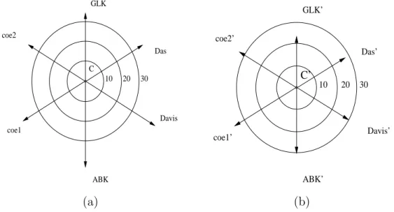
coe1 Das Davis ABK coe2 GLK C 10 20 30 ABK’ GLK’ Das’ Davis’ coe1’ coe2’ 30 20 10 C’ (a) (b)
Fig. 12. Distance between the blok and the centroid C (a) and distance between blok′ and the centroid C′ (b).
The figure 13-b shows the average and standard deviation over the six blok′
of evolvability per bit. The one over blok′
have the same shape than the mean curve over blok, only the standard deviation is different, on the average
stan-dard deviation is 0.08517 for blok and 0.08367 for blok′
. The Evolvability
Horizon is more homogeneous for the blok′
-0.4 -0.35 -0.3 -0.25 -0.2 -0.15 -0.1 -0.05 0 fitness bits position -0.4 -0.35 -0.3 -0.25 -0.2 -0.15 -0.1 -0.05 0 fitness bits position (a) (b)
Fig. 13. Average with standard deviation of evolvability per bit over the blok (a) and over the blok′ (b). The boxes below the figures indicate with a vertical line which bits are in schema S (a) and schema S′ (b).
The Olympus contains the blok′
which are the best rules known and is a subspace with unusually high fitness values easy to find as we will show in the next sections. As such, it is a potentially interesting subspace to search. However, this does not mean that the global optimum of the whole space must necessarily be found there.
5.2 Statistical Measures on the Olympus Landscape
In this section we present the results of the main statistical indicators re-stricted to the Olympus subspace.
5.2.1 Density of States and Neutrality
Figure 14-a has been obtained by sampling the space uniformly at random. The DOS is more favorable in the Olympus with respect to the whole search space (see section 3.3.1) although the tail of the distribution is fast-decaying beyond fitness value 0.5.
The neutral degree of 103 solutions randomly chosen in Olympus is depicted
in figure 14-b. Two important NN are located around fitnesses 0 and 0.5 where the neutral degree is over 80. On average the neutral degree is 51.7. For comparison, the average neutral degree for NKq landscapes with N = 64,
0 0.01 0.02 0.03 0.04 0.05 0 0.2 0.4 0.6 0.8 1 0.190 Frequency Fitness 0 20 40 60 80 100 120 0 0.2 0.4 0.6 0.8 1 Neutral Degree Fitness (a) (b)
Fig. 14. Density of states (a) and Neutral degree of solutions as a function of fitness (b) on Olympus. 103 random solutions from Olympus were evaluated on a sample
of ICs of size 104.
K = 2 and q = 2 is 21.3. Thus, the neutral degree is high on the Olympus and this should be exploited to design metaheuristics fitting the problem.
5.2.2 Fitness Distance Correlation
FDC has been calculated on a sample of 4000 randomly chosen solutions belonging to the Olympus. Results are summarized in table 7. The first six lines of this table reports the FDC where distance is calculated from one
particular solution in the blok′
. The line before last reports FDC where distance is computed from the nearest optimum for each individual belonging to the sample. The last line is the FDC, relative to euclidean distance, to the centroid
C′
. Two samples of solutions were generated: Osample, where solutions are randomly chosen in the Olympus and Csample, where each bit of a solution has probability to be ’1’ according to the centroid distribution.
With the sample based on the Olympus, the FDC is lower, meaning that
im-provement is easier for the blok′
than for the overall landscape (see section 4.2)
except for Coe1. FDC with GLK′
, ABK′
, nearest, or C′
is over the threshold −0.15. For Csample, all the FDC values are lower than on Osample. Also,
except for Coe1′
, the FDC is over the limit−0.15. This correlation shows that
fitness gives useful information to reach the local optima. Moreover, as the FDC from the centroid is high (see also figure 15), fitness leads to the centroid
C′
. We can conclude that on the Olympus, fitness is a reliable guide to drive
searcher toward the blok′
Table 7
FDC where distance is calculated from one particular solution in the blok′, the nearest, or from the centroid of blok′. Two samples of solutions of size 104 were generated: Osample and Csample.
Osample Csample GLK′ -0.15609 -0.19399 Davis′ -0.05301 -0.15103 Das′ -0.09202 -0.18476 ABK′ -0.23302 -0.23128 Coe1′ -0.01087 0.077606 Coe2′ -0.11849 -0.17320 nearest -0.16376 -0.20798 C′ -0.23446 -0.33612 0 0.1 0.2 0.3 0.4 0.5 0.6 0.7 0.8 0.9 25 30 35 40 45 Fitness Distance 0 0.1 0.2 0.3 0.4 0.5 0.6 0.7 0.8 0.9 25 30 35 40 45 Fitness Distance (a) (b)
Fig. 15. FDC scatter-plot computed with euclidean distance to the centroid C′. Two samples of solutions of size 104 were generated: Osample in (a) and Csample in (b).
5.2.3 Correlation structure analysis: ARMA model
In this section we analyze the correlation structure of the Olympus landscape using the Box-Jenkins method (see section 3.3.4). The starting solution of each random walk is randomly chosen on the Olympus. At each step one random bit is flipped such that the solution belongs to the Olympus and the fitness
is computed over a new sample of ICs of size 104. Random walks have length
approach3 is ±2/√104 = 0.02. 0 0.2 0.4 0.6 0.8 1 0 20 40 60 80 100 120 rho(s) lag s -0.1 0 0.1 0.2 0.3 0.4 0.5 0.6 0.7 0.8 0.9 0 10 20 30 40 50 60 70 rho(s) lag s (a) (b)
Fig. 16. Autocorrelation (a) and partial autocorrelation (b) function of random walk on Olympus.
Identification Figure 16 shows the estimated autocorrelation (acf) in (a)
and partial autocorrelation (pacf) in (b). The acf decreases quickly. The first-order autocorrelation is high 0.838 and it is of the same first-order of magnitude as for NK-landscapes with N = 100 and K = 7 [33]. The acf is closed to the two-standard-error bound from lag 40 and cuts this bound at lag 101 which is the correlation length. The fourth-order partial autocorrelation is close to the two-standard-error bound. The partial autocorrelation after lag 4 tapers off to zero. This suggests an AR(3) or AR(4) model. The t-test on the estimation coefficients of both model AR(3) and AR(4) are significant, but p-values of Box-Jenkins test show that residuals are not white noises. Thus, we tried to
fit an ARMA(3, 1) model. The last autoregressive coefficient α3 of the model
is close to non-significant. In order to decide the significance of this coefficient, we extracted the sequence of the 980 first steps of the walk and estimated the
model again. The t-test of α3 drops to 0.0738. So α3 is non significant and not
necessary. We thus end up with an ARMA(2, 1) model.
Estimation The results of the ARMA(2, 1) model estimation is:
yt = 0.00281 + 1.5384yt−1 − 0.5665yt−2 + ǫt − 0.7671ǫt−1
(20.4) (32.6) (13.7) (18.1)
3 All the statistic results have been obtained with the R programming environment
where yt = f (xt). The t-test statistics of the significance measure are given
below the coefficients in parentheses: they are all significant.
Diagnostic checking For the ARMA(2, 1) model estimation, the Akaide
Information Criterion (aic) is −16763.63 and the variance of residuals is
V ar(ǫt) = 0.01094. Figure 17 shows the residuals autocorrelation and p-value
of Box-Jenkins test for the estimates of the ARMA(2, 1) model. The acf of residuals are all well within the two-standard-error bound expected for h = 28. So, the residuals are not correlated. The p-value of Box-Jenkins test are quite good over 0.25. The residuals can be considered as white noises.
The value of R-square ¯R2 = 0.7050 is high and higher in comparison to the
synchronizing-CA problem [11] where ¯R2 is equal to 0.38 and 0.35.
-0.03 -0.02 -0.01 0 0.01 0.02 0.03 0.04 5 10 15 20 25 30 35 40 45 50 rho(s) lag s 0 0.2 0.4 0.6 0.8 1 0 2 4 6 8 10 12 14 p-value lag s (a) (b)
Fig. 17. Autocorrelation function of residuals (a) and p-value of Ljung-Box statistic (b) for model ARM A(2, 1).
We can conclude that the model ARMA(2, 1) accurately fits the fitness val-ues given by random walks over the Olympus Landscape. The high correlation shows that a local search heuristic is adequate to find good rules on the Olym-pus. An autoregressive model of size 2 means that we need two steps to predict the fitness value; so, as suggested by Hordijk, it would be possible to construct more efficient local search taking into account this information. The moving average component has never been found in other landscape fitness analysis. What kind of useful information does it give? Maybe information on nature of neutrality. Future work should study those models in more detail.
5.2.4 Fitness Cloud and NSC
Figure 18 shows the scatterplot and the segments {S1, S2, ..., Sm−1} used to
slope, it seems easy for a local search heuristic to reach fitness values close to 0.6. A comparison of this fitness cloud with the one shown in figure 5 (where the whole fitness landscape was considered, and not only the Olympus) is illuminating: if the whole fitness landscape is considered, then it is “hard” to find solutions with fitness up to 0.5 ; on the other hand, if only solutions belonging to the Olympus are considered, the problem becomes much easier : it is now “easy” to access to solutions with fitness greater than 0.5.
0 0.1 0.2 0.3 0.4 0.5 0.6 0.7 Fitness 0 0.1 0.2 0.3 0.4 0.5 0.6 0.7 0.8 Fitness 0 0.1 0.2 0.3 0.4 0.5 0.6 0 0.1 0.2 0.3 0.4 0.5 0.6 0.7 0.8 0 0.1 0.2 0.3 0.4 0.5 0.6 0.7 Fitness Fitness
Fig. 18. Fitness Cloud and Scatterplot used to calculate the NSC value on Olympus.
5.3 Genetic Algorithms on the Olympus Landscape
In this section, we use different implementations of a genetic algorithm to con-firm our analysis of the Olympus and to find good rules to solve the Majority problem. All implementations are based on a simple GA used by Mitchell et al. in [5].
A population of 200 rules is used and fitness is computed by the success rate on unbiased sample of ICs. New individuals are first evaluated on sample of size
103. At each generation, a new sample of size 103is generated. If an individual
stays in the population during n generations, its fitness is computed from a
sample of size 103n which corresponds to the cumulative sample of ICs. In all
cases, initialization and mutation are restricted to the Olympus. In order to obtain, on average, one bit mutation per individuals on Olympus, the mutation probability per bit is 1/77. One point crossover is used with rate 0.6. We use three implementations of this GA : the Olympus based GA (oGA), the Centroid based GA (cGA) and the Neutral based GA (nGA). The oGA allows to test the usefulness of searching in the Olympus, the cGA tests the efficiency of searching around the centroid and the nGA exploits the considerable neutrality of the landscape.
Initial population For ’Olympus’ and ’Neutral’ based GAs, the initial pop-ulation is randomly chosen in the Olympus. For cGA, the initial poppop-ulation is generated according to the centroid: probability to have ’1’ at a given bit
position is given by C′ value at the same position. In the same way, if one bit
is mutated, its new value is generated according to C′
.
Selection schema oGA and cGA both use the same selection scheme as
in Mitchell et al.. The top of 20 % of the rules in the population, so-called elite rules, are copied without modification to the next generation and the remaining 80 % for the next generation were formed by random choice in the elite rules. The selection scheme is similar to the (µ+λ) selection method. The nGA uses tournament selection of size 2. It takes into account the neutrality of the landscape: if the fitnesses of two solutions are not statistically different using the t-test of 95 % of confidence, we consider that they are equal and
choose the individual which is the more distant from the centroid C′
; this choice allows to spread the population over the neutral network. Otherwise the best individual is chosen. nGA uses elitism where the top 10 % of different rules in the population are copied without modification.
Performance Each GA run lasts 103 generations and 50 independent runs
were performed. For each run, we have performed post-processing. At each
generation, the best individuals are evaluated on new sample of 104 ICs and
the average distance between all pairs of individuals is computed. Best and average performances with standard deviation are reported in table 8. We also computed the percentage of runs which are able to reach a given fitness level and the average number of generations to reach this threshold (see figure 19).
Table 8
GA performances computed on sample of size 104.
GA Average Std Deviation Best oGA 0.8315 0.01928 0.8450 cGA 0.8309 0.00575 0.8432 nGA 0.8323 0.00556 0.8472
All GAs have on average better performances than the optima find by hu-man or by genetic programming. As expected, searching in the Olympus is useful to find good rules. All the GAs have nearly the same average perfor-mances. However, standard deviation of ’Olympus’ is four times larger than standard deviation of ’Centroid’. As it is confirmed by the mean distance be-tween individuals, the cGA quickly looses diversity (see fig. 20). On the other hand, ’Neutral’ GA keep genetic diversity during runs. Figure 19 shows that for the most interesting threshold over 0.845, ’Neutral’ have more runs able
0 0.2 0.4 0.6 0.8 1 0.8 0.81 0.82 0.83 0.84 0.85 0.86 0.87 Percent of runs Fitness cGA oGA nGA 0 100 200 300 400 500 600 700 800 900 0.8 0.81 0.82 0.83 0.84 0.85 0.86 0.87 Average generation Fitness cGA cGA nGA (a) (b)
Fig. 19. Statistics percentage of runs (a) and number of generations (b) for the evo-lutionary emergence of CAs with performances exceeding various fitness thresholds.
to overcome the threshold (3/50) than ’Olympus’ (1/50) or ’Centroid’ (0/50). Even though we cannot statistically compare the best performance of different GAs, the best rule was found by the nGA with performance of 0.8472 to be compared to the second best rule Coe1.
0 5 10 15 20 25 30 35 40 0 100 200 300 400 500 600 700 800 900 1000 Distance Generations cGA oGA nGA
Fig. 20. Average hamming distance between individuals of population as a function of generation.
These experimental results using GAs confirm that it is easy to find good rules in the Olympus Landscape. During all the 50 independent runs, we find a lot of different CAs with performance over 0.82: 3642 for oGA, 1854 for cGA and 11437 for nGA. A ’low’ computational effort is needed to obtain such CAs. A run takes about 8 hours on PC at 2 GHz. Taking the neutrality into account allows to maintain the diversity of the population and increases the chance to reach rules with high performance.
6 Conclusions
Cellular automata are capable of universal computation and their time evo-lution can be complex and unpredictable. We have studied CAs that perform the computational Majority task. This task is a good example of the phe-nomenon of emergence in complex systems is. In this paper we have taken an interest in the reasons that make this particular fitness landscape a difficult one. The first goal was to study the landscape as such, and thus it is ideally independent from the actual heuristics used to search the space. However, a second goal was to understand the features a good search technique for this particular problem space should possess. We have statistically quantified in various ways some features of the landscape and the degree of difficulty of optimizing. The neutrality of the landscape is high, and the neutral network topology is not completely random. The main observation was that the land-scape has a considerable number of points with fitness 0 or 0.5 which means that investigations based on sampling techniques on the whole landscape are unlikely to give good results.
In the second part we have studied the landscape from the top. Although it has been proved that no CA can perform the task perfectly, six efficient CAs for the majority task have been found either by hand or by using heuristic methods, especially evolutionary computation. Exploiting similarities between these CAs and symmetries in the landscape, we have defined the Olympus landscape as a subspace of the Majority problem landscape which is regarded
as the ”heavenly home” of the six symmetric of best local optima known (blok′
). Then, we have measured several properties of the Olympus landscape and we have compare with those of the full landscape, finding that there are less solutions with fitness 0. FDC shows that fitness is a reliable guide to drive a
searcher toward the blok′
and its centroid. An ARMA(2, 1) model has been used to describe the fitness/fitness correlation structure. The model indicates that local search heuristics are adequate for finding good rules. Fitness clouds and nsc confirm that it is easy to reach solutions with fitness higher than 0.5. Although it is easier to find relevant CAs in this subspace than in the complete landscape, there are structural reasons that prevents a searcher from finding overfitted GAs in the Olympus. Finally, we have studied the dynamics and performances of three Genetic Algorithms on the Olympus in order to confirm our analysis and to find efficient CAs for the Majority problem with low computational effort.
Beyond this particular optimization problem, the method presented in this paper could be generalized. Indeed, in many optimization problems, several efficient solutions are available, and we can make good use of this set to design an ”Olympus subspace” in the hope of finding better solutions or finding good solutions more quickly.