HAL Id: cea-02434032
https://hal-cea.archives-ouvertes.fr/cea-02434032
Submitted on 18 Mar 2020
HAL is a multi-disciplinary open access archive for the deposit and dissemination of sci-entific research documents, whether they are pub-lished or not. The documents may come from teaching and research institutions in France or abroad, or from public or private research centers.
L’archive ouverte pluridisciplinaire HAL, est destinée au dépôt et à la diffusion de documents scientifiques de niveau recherche, publiés ou non, émanant des établissements d’enseignement et de recherche français ou étrangers, des laboratoires publics ou privés.
Indirect method of measuring glass temperature in a
Cold Crucible Induction Melter
G. Barba Rossa, E. Sauvage, P. Brun
To cite this version:
G. Barba Rossa, E. Sauvage, P. Brun. Indirect method of measuring glass temperature in a Cold Crucible Induction Melter. XVIII International UIE - Congress on Electrotechnologies for Material Processing, Jun 2017, Hanovre, Germany. �cea-02434032�
XVIII International UIE-Congress
Electrotechnologies for Material Processing
Hannover (Germany), June 6-9, 2017
Indirect method of measuring glass temperature in a Cold
Crucible Induction Melter
G. Barba Rossa, E. Sauvage, P. Brun
Abstract
This study concerns the control and optimization of the vitrification process of nuclear waste in a Cold Crucible Induction Melter (CCIM). A new method was developed for the control of glass temperature in the crucible, based on the precise measurement of heat flux through a water-cooled rod immersed in the glass melt. The measuring rod is separated from the flowing hot glass by a cold glass “skull”, ensuring much lower exposure to corrosive conditions than classical thermocouple sensors. This heat flux measurement enables a precise estimation of the glass temperature using a newly designed correlation formula between heat flux and glass temperature. Dimensioning of the measurement rod – i.e. its size and cooling water supply – was made possible by running coupled 3D numerical simulations of fluid flow, heat transfers and electromagnetics in the CCIM.
Introduction
Material processing involving Cold Crucible Induction Melters needs precise temperature control using sensors that can withstand highly corrosive conditions and relatively strong harmonic magnetic fields. Until now, most temperature measurements have been carried out by means of thermocouple sensors embedded in “glove fingers” made of noble materials able to tolerate corrosive hot glass flows. In such a design, the fingers have to be sufficiently long and thin to eliminate perturbations induced by heat conduction towards the water-cooled rod propping them up. The study described here focused on the design and testing of an indirect temperature measurement technique based on heat flux measurement. A temperature estimator was derived using multiphysics modeling of the CCIM, taking into account direct electromagnetic induction inside the melt, glass flow, and heat transfers.
1. CCIM modelling and estimator design
1.1. Cold Crucible Induction Melting
Cold Crucible Induction Melters are cooled crucibles in which processed materials are heat-treated by direct electromagnetic induction. In the vitrification process of nuclear waste, the glass mixture is vigorously stirred with an immersed rotating agitator shaft to obtain atomic scale entrapment of nuclear wastes, and both thermal and chemical homogenization. The use of cold crucible induction melters is suitable for processing extremely corrosive materials that require high elaboration temperatures. Almost every part of the metallic crucible is water-cooled, and thus becomes coated with a cold protective layer usually called a “glass skull”. Rather than being submitted to high temperatures, these cooled elements undergo strong heat transfers from the glass melt to the cooling water.
1.2. Multiphysics modelling
The glass mixture is considered as a local non-polarizable and non-magnetic linear isotropic conductor. The Maxwell equations are written in the quasi-magnetostatic approximation, using the 𝑨 − 𝑉 potentials formulation, and are solved in the frequency domain. Enforcing Coulomb gauge, the induction problem is reduced to the following Maxwell-Ampère and charge conservation equations:
𝛻2𝑨 = 𝜇
0𝜎(𝛻𝑉 + 𝑖2𝜋𝑓𝑨) (1.1)
𝛻 ⋅ (𝜎(𝛻𝑉 + 𝑖2𝜋𝑓𝑨)) = 0 (1.2)
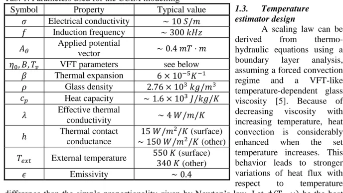
The parameters appearing in all the equations are grouped in Tab. 1. For the sake of simplicity, only typical values are given since most of the parameters related to glass are temperature-dependent. The external oscillating magnetic field produced by the surrounding inductor is modelled by a uniform vertically oriented field, using suitable Dirichlet boundary conditions for the vector potential on the cylindrical lateral boundary of the melt:
𝑨 = 𝐴𝜃𝒆𝜽 (1.3)
where 𝒆𝜽 is the orthoradial unit vector, and homogeneous Neumann boundary conditions are assumed on other boundaries [1, 2]. A non-homogeneous Neumann boundary condition for the scalar potential on every boundary ensures zero face-normal currents (the glass skull is considered to be a perfect electrical insulator):
𝜕𝑉
𝜕𝑛 = −𝑖2𝜋𝑓𝑨 ⋅ 𝒏 (1.4)
where 𝒏 is the outward pointing normal unit vector [3]. Thermo-hydraulic modelling assumes an incompressible and laminar flow of glass, which is considered as a Newtonian fluid with temperature-dependent viscosity following the Volgel-Fulcher-Tammann (VFT) law:
𝜂(𝑇) = 𝜂0 exp (𝑅(𝑇−𝑇𝐵
𝑣)) (1.5)
The Navier-Stokes equations are written under the Boussinesq approximation to account for natural convection, and the Rosseland diffusion approximation for internal radiation is applied to the energy equation. Viscous dissipation is ignored, leading to the following steady-state set of equations for velocity 𝒖, pressure 𝑝 and temperature 𝑇 [4]:
𝛻 ⋅ 𝒖 = 0 (1.6)
𝛻𝒖 ⋅ 𝒖 = −𝛻𝑝 + 𝛻 ⋅ (𝜂(∇𝒖 + ∇𝒖𝑇)) − 𝛽(𝑇 − 𝑇
𝑟𝑒𝑓)𝒈 (1.7)
𝜌𝑐𝑝𝒖 ⋅ 𝛻𝑇 = 𝛻 ⋅ (𝜆∇𝑇) +𝜎2‖𝛻𝑉 + 𝑖2𝜋𝑓𝑨‖2 (1.8)
where 𝑇𝑟𝑒𝑓 is an arbitrary reference temperature and ‖⋅‖ denotes the canonical Hermitian norm. The source term in the equation for temperature is the time-averaged Joule power density. A no-slip condition is prescribed for the fluid velocity on all boundaries except for the surface of the melt, subjected to Marangoni stress. Eventually, the temperature field must satisfy heat flux equilibrium with the exterior on every boundary:
Tab. 1. Parameters used for the CCIM modelling
1.3. Temperature estimator design
A scaling law can be derived from thermo-hydraulic equations using a boundary layer analysis, assuming a forced convection regime and a VFT-like temperature-dependent glass viscosity [5]. Because of decreasing viscosity with increasing temperature, heat convection is considerably enhanced when the set temperature increases. This behavior leads to stronger variations of heat flux with respect to temperature difference than the simple proportionality given by Newton’s law. Let 𝜙(𝑇ℎ, 𝜔) be the heat flux received by any cooled sensor immersed in the melt for a set glass hot temperature 𝑇ℎ (around mean temperature 〈𝑇ℎ〉) and stirring rotational speed 𝜔. The boundary layer analysis, not shown in this paper, leads to:
𝜙(𝑇ℎ, 𝜔) = (𝑇ℎ𝛼−𝑇𝑣) 1+𝛾
𝜔1⁄ 2 (1.10)
where 𝛾 depends only on the glass VFT parameters and the mean set temperature (𝑅 stands for the universal gas constant):
𝛾 =3𝑅(〈𝑇𝐵
ℎ〉−𝑇𝑣) (1.11)
and 𝛼 is a certain scaling constant depending on the sensor geometry and other glass properties. Hence, the temperature estimator is defined by inverting the scaling law:
𝑇ℎ ̅̅̅ = 𝑇𝑣+ 𝛼 (𝜙𝜔−1 2⁄ ) 1 1+𝛾 ⁄ (1.12)
Equation (1.12) is only valid for steady-states. The following section evaluates the scaling constant 𝛼 for a particular sensor design using 3D coupled numerical simulation of the CCIM.
2. Sensor design and numerical simulation
2.1. Heat flux sensor
In the design described here, the heat flux sensor is a part of a cylindrical water-cooled rod made of stainless steel and immersed in the melt. The heat flux received by the measurement rod is computed from the temperature difference between incoming and outgoing cooling water. An accurate heat flux measurement needs a sufficiently high water temperature difference, but must prevent any vaporization inside the sensor. The results of 3D
Symbol Property Typical value
𝜎 Electrical conductivity ∼ 10 𝑆/𝑚 𝑓 Induction frequency ∼ 300 𝑘𝐻𝑧 𝐴𝜃 Applied potential
vector ∼ 0.4 𝑚𝑇 ⋅ 𝑚
𝜂0, 𝐵, 𝑇𝑣 VFT parameters see below 𝛽 Thermal expansion 6 × 10⁻⁵𝐾−1 𝜌 Glass density 2.76 × 10³ 𝑘𝑔/𝑚3 𝑐𝑝 Heat capacity ∼ 1.6 × 10³ 𝐽/𝑘𝑔/𝐾 𝜆 Effective thermal conductivity ∼ 4 𝑊/𝑚/𝐾 ℎ Thermal contact conductance 15 𝑊/𝑚2/𝐾 (surface) ∼ 150 𝑊/𝑚2/𝐾 (other) 𝑇𝑒𝑥𝑡 External temperature 550 𝐾 (surface) 340 𝐾 (other)
coupled numerical simulations of the CCIM shown hereafter enabled a precise estimation of the heat flux, thus ensuring a proper sizing of the sensor in terms of cooling rate.
2.2. Simulation strategy and results
Equations (1.1), (1.2), (1.6), (1.7) and (1.8) can be solved simultaneously with a finite volume scheme using ANSYS ® Fluent. Equations (1.1) and (1.2) – written here for complex amplitudes – were split into 8 real scalar equations and added to the software workflow using User Defined Functions. Couplings were solved with a segregated method until global convergence was reached. The embedded Multiple Reference Frame model was used to solve the stirrer steady rotational motion [6]. For a given value of stirring intensity 𝜔 ≈ 5 𝑟𝑎𝑑/𝑠, tuning the value of applied vector potential 𝐴𝜃 enabled different values of glass temperature inside the melt to be reached, ranging from 1200 °𝐶 to 1300 °𝐶. For each temperature, the total heat flux across the measuring rod boundary was computed.
The glass used in the experiment was a French borosilicate simulant glass for the vitrification of fission products. Precise rheological measurements with varying temperatures were carried out on a small sample of glass. The glass was found to follow the Vogel-Fulcher-Tammann law very accurately in the temperature range under study (see Fig. 1) with parameters:
𝜂0 = 1.16 × 10⁻² 𝑃𝑎 ⋅ 𝑠, 𝐵 = 3.32 × 10⁴ 𝐽/𝑚𝑜𝑙, 𝑇
𝑣 = 586 °𝐶 (2.1)
leading to the scaling law exponent 𝛾 = 2.00. Numerical simulations show very clearly that the behavior of heat flux with respect to the set hot temperature is in good agreement with the analytical scaling law, setting the scaling constant 𝛼 ≈ 55.9 𝑆𝐼 and 〈𝑇ℎ〉 = 1250 °𝐶 (see Fig. 1 and 2).
Fig. 2: Numerical simulation of the CCIM – horizontal cross section colored by Joule power density, vertical plane colored by temperature and heat flux sensor envelope
in gray 0 2 4 6 8 10 12 14 16 2.50 3.00 3.50 4.00 4.50 5.00 5.50 6.00 1150 1200 1250 1300 1350 Dy n am ic al visc os ity (P a. s) He at fl u x th rou gh th e senso r (kW)
Prescribed hot temperature (°C)
VFT law
Heat flux from Equation (1.10) Heat flux from simulation Viscosity measurements
Fig. 1: Heat flux comparison between numerical results and analytical scaling law - viscosity change on the temperature
3. Experimental validation
3.1. Experimental setup
The experiment consisted in the melting of around 300 kg of glass simulant. The CCIM was instrumented with both the heat flux sensor and a thermocouple sensor. The experiment was programmed to last 24 hours, and automatic measurements of temperature and heat flux were performed every 5 minutes. Temperature control was achieved with a PID controller governing the Joule power injected into the melt by the surrounding inductor. Different temperatures were set for the melt, starting from a temperature of 1290 °𝐶 and down to 1200 °𝐶 with constant stirring rotation speed ≈ 5 𝑟𝑎𝑑/𝑠 . Each 10°𝐶 decrease in the command was followed by a stabilization period of at least one hour. The glass melt was then reheated up to 1300 °𝐶. After stabilization, stirring intensity was decreased step by step down to 2 𝑟𝑎𝑑/𝑠 with stabilization plateaus.
3.2. Results
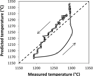
Fig. 3 shows the comparison between the glass temperature given by the thermocouple sensor and predicted temperature 𝑇̅̅̅ obtained ℎ from heat flux measurements. A good agreement can be observed, with less than 20°C deviation during the first sequence, even during transient regimes following the change in set temperature between plateaus. A larger deviation can be seen when heating the melt back to higher temperatures, due to a strong imbalance between injected Joule power and heat fluxes from the melt to the cold crucible. For the second sequence, the behavior of the temperature estimator was satisfactory but showed a larger deviation, up to 40°C for the lowest stirring intensity. This overestimation could be due to the fact that natural convection is no longer negligible for low rotational speeds. The contribution of free convection to the heat flux received by the sensor was not accounted for in the boundary layer analysis, because of the assumption of a forced convection regime. This assumption was however valid for high rotational speeds, for which the Richardson number in the melt 𝑅𝑖 ∝ 𝜔−2 was low enough (about 2 × 10⁻²).
Conclusions
In this study, a Model and Simulation-based Systems Engineering approach was used to design a new indirect method of measuring glass temperature in a Cold Crucible Induction Melter used for nuclear waste vitrification. The temperature was computed from real-time measurements of the heat flux received by a cooled sensor immersed in the melt, able to withstand extremely corrosive conditions. The temperature estimator was derived from an analytical and numerical study of the magneto-thermo-hydraulic problem and showed a good agreement with the experimental data collected on a melting experiment where glass was vigorously stirred using a mechanical cooled agitator. Unlike classical thermocouple sensors,
1150 1170 1190 1210 1230 1250 1270 1290 1310 1330 1350 1150 1200 1250 1300 1350 Pr e d ict e d t e m p e ra tu re ( °C) Measured temperature (°C)
Fig. 3: Comparison between measured glass temperature and the estimator
which need special costly finger gloves to withstand a hot glass flow, the sensor was reduced to a simple water-cooled tube made of steel. The deviation observed for low stirring rotation speeds in the experiments could be eliminated by using a boundary layer analysis in the mixed heat convection regime, thus accounting for free convection effects.
Acknowledgements
The authors would like to thank the Joint Vitrification Lab (LCV), Areva and EDF for the financial support of this work.
References
[1] Badics, Z.: Transient eddy current field of current forced three-dimensional conductors. IEEE Transactions on magnetics, Vol. 28, 1992, pp. 1232–1234.
[2] Biro, O., Preis, K.: On the use of the magnetic vector potential in the finite element analysis of
three-dimensional eddy currents. IEEE Transactions on magnetics, Vol. 25, 1989, pp. 3145–3159.
[3] Beckstein, P., Galindo, V., Gerbeth, G.: Free-surface dynamics in the ribbon growth on substrate (rgs)
process. Proceedings of the International Conference on Heating by Electromagnetic Sources, Padua, 2016, pp.
127-134.
[4] Bird, R. B., Stewart, W. E., Lightfoot, E. N.: Transport Phenomena. John Wiley & Sons, 2007, 905 pp. [5] Barba Rossa, G., Sauvage, E.: Transfert thermique d’un fluide à viscosité thermo-dépendante vers une paroi
refroidie. Congrès Français de Thermique, Toulouse, 2016, 36.
[6] ANSYS ® Fluent, Release 15.0, Help System, Theory Guide, ANSYS, Inc.
Authors
Barba Rossa, Guillaume Sauvage, Emilien
CEA, DEN, DE2D, SEVT, LDPV CEA, DEN, DE2D, SEVT, LDPV
Centre de Marcoule Centre de Marcoule
F-30207 Bagnols-sur-Cèze F-30207 Bagnols-sur-Cèze
E-mail: guillaume.barbarossa@cea.fr E-mail: emilien.sauvage@cea.fr Brun, Patrice
CEA, DEN, DE2D, SEVT, LDPV Centre de Marcoule
F-30207 Bagnols-sur-Cèze E-mail: patrice.brun@cea.fr