Adaptive estimation of acoustic normal modes

The

RESEARCH LABORATORY

of

ELECTRONICS

at the

MASSACHUSETTS INSTITUTE OF TECHNOLOGY

CAMBRIDGE, MASSACHUSETTS 02139

Adaptive Estimation of Acoustic Normal Modes

Kathleen E. Wage

RLE Technical Report No. 586

Adaptive Estimation of Acoustic Normal Modes

Kathleen E. Wage

RLE Technical Report No. 586

October 1994

The Research Laboratory of Electronics

MASSACHUSETTS INSTITUTE OF TECHNOLOGY

CAMBRIDGE, MASSACHUSETTS 02139-4307

This work was supported in part by a Clare Boothe Luce Fellowship and in part by the University

of California - Scripps ATOC Agreement PO 10037359.

Adaptive Estimation of Acoustic Normal Modes

by

Kathleen E. Wage

Submitted to the MIT Department of Electrical Engineering and Computer Science

and to the WHOI Department of Applied Ocean Science and Engineering

in partial fulfillment of the requirements for the degree of

Master of Science

Abstract

Normal mode theory provides an efficient description of signals which propagate axially in

the SOFAR channel and are detectable at long ranges. Mode amplitudes and their second

order statistics are useful in studies of long-range acoustic propagation and for applications

such as Matched Mode Processing (MMP) and Matched Field Tomography (MFT). The

purpose of this research is to investigate techniques for estimating the average power in the

modes of a signal given pressure measurements from a vertical line array.

This thesis develops the problem of mode estimation within a general array processing

framework which includes both deterministic and stochastic characterizations of the modal

structure. A review of conventional modal beamforming indicates that these methods

pro-vide poor resolution in low signal-to-noise ratio environments. This is not surprising since

standard estimation techniques rely on minimizing a squared error criterion without regard

to the ambient noise. The primary contribution of this thesis is an adaptive estimator for

coherent modes that is based on a method suggested by Ferrara and Parks for array

pro-cessing using diversely-polarized antennas. Two formulations of the adaptive method are

investigated using a combination of analytical techniques and numerical simulations. The

performance evaluation considers the following issues: (i) power level of the noise, (ii)

or-thogonality of the sampled modeshapes, (iii) number of data snapshots, and (iv) coherence

of the signal. The new approach is fundamentally different from other modal estimators

such as those used in MMP because it is data-adaptive and maximizes the received power

instead of minimizing the squared error. As a result, the new methods perform significantly

better than least squares in high noise environments. Specifically, the Ferrara/Parks

formu-lations are able to maintain nulls in the modal spectrum since they do not suffer the bias

error that significantly affects the least squares processor.

A second contribution of the thesis is an extension of the coherent estimator to facilitate

estimation of phase-randomized modes. Although the results of this work are preliminary,

the extended formulation appears to offer several advantages over least squares in certain

cases.

Thesis Supervisor: Arthur B. Baggeroer

Acknowledgements

First, I thank God for the many blessings that have enriched my life and ultimately made this work possible.

I thank my advisor, Prof. Arthur Baggeroer, for suggesting this area of research and for providing invaluable technical guidance along the way. Thanks also to Brian Sperry for many useful discussions regarding this research.

I have learned a great deal from my colleagues in the Digital Signal Processing Group. Their help and friendship is much appreciated. In particular, I am indebted to Steve Isabelle for his thoughtful advice and encouragement.

I consider my experiences as a teaching assistant to be one of the most valuable aspects of the past three years. It has been a true privilege to work with John Buck, Prof. Steve Leeb, Prof. Alan Oppenheim, Stephen Scherock, and Andy Singer.

Many people have provided the necessary doses of humor, encouragement, and e-mail that have helped me maintain my sanity in graduate school. For their kindness and friend-ship I am especially grateful to: Amy Troutman, Emily Parkany, Dr. Cristi Bell-Huff, Melissa Caldwell, Aradhana Narula, Karin Knoll, Dr. Ellen Livingston, Mark Allen, and Susie Wee. A special thanks to the Knoxville-based moral support engineering firm of

"Dr." Kathy and Steve Drevik for their southern hospitality.

At this stage of my life, no thesis can be complete without acknowledging all of the people who got married while I was working on it. So a special thanks (and best wishes!) to the following couples who provided me with some welcome weekends away from MIT: Amanda and Randy, Kathy and Steve, Pam and David, Lizette and Frank, Becky and Mike, Karen and Randy, Cristi and John, Melissa and Eric, and Traci and Ernesto.

Finally, I am eternally grateful to my parents, Jim and Virginia Wage, for their love and support. It is with sincere thanks that I dedicate this thesis to them.

Funding for this work was provided by a Clare Boothe Luce Fellowship (1991-1992) and the University of California - Scripps ATOC Agreement, PO#10037359.

Contents

2.1 Ocean Acoustic Waveguide ...

2.2 Normal Mode Representation of Narrowband Signals ... 2.2.1 Modal Propagation in a Range-Independent Waveguide 2.2.2 Modal Propagation in a Range-Dependent Waveguide 2.2.3 Modal Propagation in a Random Waveguide ... 2.3 Problem Formulation ...

2.4 Important Considerations in Modal Array Processing ... 2.4.1 Ambient Noise ...

2.4.2 Modal Orthogonality ...

2.4.3 Estimation of the Covariance Matrix ... 2.4.4 Signal Coherence ... 2.4.5 Performance Measures ... 3 4 5 7 10 10 13 14 15 ... .15 ... .17 ... .18 . . . 22 ... .23 ... .24 ... .26 . . . 27 ... .28 ... .30 ... .31 ... .32

.. . . . .

.

3 Least Squares Methods 3.1 Standard Least Squares ... 3.1.1 Ambient Noise ... 3.1.2 Modal Orthogonality .... 3.1.3 Estimated Covariance Issues 3.1.4 Signal Coherence ... 3.2 Summary ... 4 Adaptive Estimation of Coherent Modes 4.1 Minimum Variance Modal Estimator . . 4.1.1 Ambient Noise ... 4.1.2 Modal Orthogonality ... 4.1.3 Estimated Covariance Issues . . 4.1.4 Signal Coherence ... 4.2 MUSIC Modal Estimator ... 4.2.1 Ambient Noise ... 4.2.2 Modal Orthogonality ... 4.2.3 Estimated Covariance Issues . . . 4.2.4 Signal Coherence ... 4.3 Summary ... 5 Adaptive Estimation of Incoherent Modes 5.1 Modified Minimum Variance Formulation 5.2 Summary ... 6 Conclusion 6.1 Sum m ary . . .... .. ... .. ... . ... . .. . . .. . 6.2 Suggestions for Further Research ... A Fisher Information Matrix for Modal Estimation B Mean and Variance of the Least Squares Power Estimates 34 . . . 35 ... 39 . . . 41 . . . 44 . . . 45 . . . 45 47 . . . 49 . . . 55 . . . 57 . . . 59 . . . 63 . . . 65 ... ... 71 . . . 73 . . . 74 . . . 76 . . . 77 79 79 86 88 88 89 91 93 2.5 Summary ... ...

C Mean and Variance of the MV Power Estimates 95

D Mean and Variance of the MUSIC Power Estimates 97

List of Figures

2-1 Model of an ocean environment . . . 16

2-2 Data acquisition and pre-processing ... ... . 17

2-3 Idealized range-independent waveguide . . . 18

2-4 Sound speed profile and modeshapes for the deep water waveguide .... . 20

2-5 Simulation array for the deep water waveguide ... ... . 29

2-6 Modeshape correlation for the deep water waveguide ... 30

2-7 Degrees of freedom for the simulation array ... ... . 31

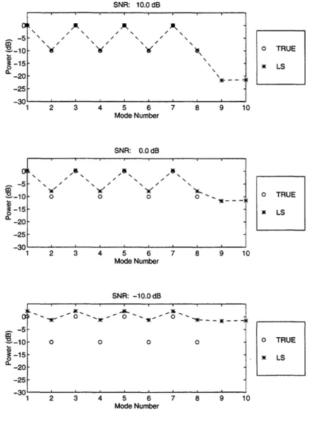
3-1 Least squares power estimates for the deep water example ... . 37

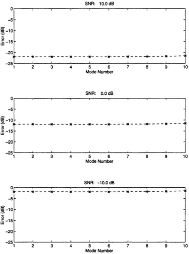
3-2 Error in least squares power estimates for the deep water example .... . 39

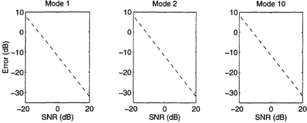
3-3 Error vs. SNR for modes 1, 2, and 10 of the deep water waveguide. Ambient noise consists of white sensor noise only ... 40

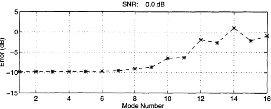
3-4 Error vector for the 16-mode example using the deep water waveguide . . . 42

3-5 Total error vs. number of modes to estimate for the deep water example . . 43

3-6 Bias error vs. number of snapshots for mode 1. Predicted and Monte Carlo results for the LS estimator are shown ... 45

3-7 Variance vs. number of snapshots for mode 1. Predicted and Monte Carlo results for the LS estimator are shown along with the Cramer Rao bound.. 46

4-1 Minimum variance power estimates for the deep water example ... . 52

4-2 Error in minimum variance power estimates for the deep water example . . 55

4-3 Error vs. SNR for modes 1, 2, and 10 of the deep water waveguide. Ambient noise consists of white sensor noise only. Both MV and LS errors are shown for the ideal covariance case. Note that the vertical scale for mode 10 is different than for modes 1 and 2 ... 56

4-4 Error vector for the 16-mode example using the deep water waveguide . . 57

4-5 Total error vs. number of modes to estimate for the deep water example. Two cases are shown: the top plot displays the 0 dB SNR results and the bottom plot displays the -10 dB SNR results ... 58

4-6 Example of global localization problem for the MV estimator: 15 modes estimated at -10 dB SNR ... 60

4-7 Peaks of the minimum variance power spectrum for the 15-mode estimate at two SNR levels: 0 dB and -10 dB ... 60

4-8 Bias error vs. number of snapshots for mode 1. Predicted and Monte Carlo results are shown ... 62

4-9 Variance vs. number of snapshots for the MV estimator. Predicted and Monte Carlo simulation values are shown. The Cramer Rao bound is given for reference ... 63

4-10 Total error vs. coherence for the Ferrara/Parks MV formulation ... . 64

4-11 MUSIC power estimates for the deep water example ... ... . 69

4-12 Error in MUSIC power estimates for the deep water example ... . 71

4-13 Error vs. SNR for modes 1, 2, and 10 of the deep water waveguide. Ambient noise consists of white sensor noise only. MUSIC, MV, and LS error curves are shown for the ideal covariance case. Note that the vertical scale for mode 10 differs from the one used for modes 1 and 2 ... 72

4-14 Error vector for the 16-mode example using the deep water waveguide. MU-SIC, MV, and LS results are shown ... ... . 73

4-15 Total error vs. number of modes to estimate for the deep water example. Results for two input SNR's (0 dB and -10 dB) are shown ... 74

4-16 Error vs. number of snapshots for mode 1. Predicted and Monte Carlo results are shown for all three estimators ... 76

4-17 Variance vs. number of snapshots for the MUSIC estimator ... 77

4-18 Total error vs. coherence for the Ferrara/Parks MUSIC formulation .... . 78

5-1 Estimation Error for Partially Incoherent Mode Example ... . 82

5-2 Total Error vs. Coherence for the Modified MV Algorithm. SNR=0 dB... 85 5-3 Total Error vs. Coherence for the Modified MV Algorithm. SNR=10 dB. . 86

Chapter 1

Introduction

1.1

Motivation

The ocean is an extremely efficient channel which is capable of transmitting low frequency sound over long distances. Sound waves refract towards regions of lower velocity, therefore a minimum in sound speed creates an acoustic channel. For example, sound propagating downward from a source bends back toward the channel axis (depth of minimum sound speed). Once it passes through the axis on an upward path, it begins to bend away from the surface. In this fashion, sound is effectively trapped in a duct and can propagate from a source to a receiver hundreds or even thousands of kilometers away. In the deep ocean a minimum sound speed (occurring at approximately 1 km below the surface) defines the ocean acoustic waveguide which is also known as the SOund Fixing And Ranging (SOFAR) channel [1].

Normal mode theory provides an efficient description of low frequency sound traveling along refracted paths in the SOFAR channel. Coherent interference of a family of rays that share the same phase speed creates a standing wave (or mode) in depth. The modes form a complete set of orthogonal basis functions in the vertical. As a result, the sound pressure at any receiver point in the waveguide consists of a weighted sum of normal modes. The phase speed specifies the turning depths of the rays and determines the vertical extent of each corresponding mode. High order modes have low phase speeds and are associated with families of rays that intersect the surface or bottom boundaries. Since these modes suffer severe losses, the lower order or axial modes contain most of the signal energy at long ranges. The normal mode representation is efficient because only a subset of modes are

required to describe a signal at a significant distance from its source.

Normal mode theory offers more than just a convenient description of acoustic signals. Since the modes span different vertical sections of the water column, they each provide specific information about the sound source and the propagation path. Consequently, the normal mode decomposition is useful in several applications such as source localization and acoustic tomography. For example, recent papers indicate that source range and depth information may be obtained through matched field beamforming using the modal coeffi-cients (or weights) [2, 3, 4]. In the literature this technique is known as Matched Mode Processing (MMP).1 In another application, acoustic tomography is used to measure the speed of sound in the ocean. Normal modes are useful in this regard since modal group delays depend on the sound speed. Provided the mode arrivals can be reliably tracked, re-searchers can obtain estimates of the sound speed. In turn, these estimates provide valuable information about the channel. Note that one of the fundamental problems associated with both of the aforementioned applications is the detection and estimation of the modes in an acoustic signal. The purpose of this research is to explore techniques for modal estimation. Receivers capable of extracting the underlying modal structure typically consist of ver-tical arrays of sensors. One characteristic of acoustic propagation is that modes travel with different group velocities. Note that the group delays associated with the higher order modes may permit resolution on the basis of arrival time.2 Temporal resolution of the lower order modes, however, is not usually possible since their group delays are almost identical. Instead, an array can resolve these axial modes based on differences in their spatial distri-butions. This thesis focuses on array processing algorithms for estimation of the low order modes because they remain the most energetic at long ranges from the source.

The success of the applications described above depends on accurate modeling of acous-tic propagation. Many issues concerning transmissions over long distances in the ocean remain unresolved. Two of these issues, mode coherence and mode coupling, are particu-larly relevant to this thesis since they affect the mode estimation problem.

Mode coherence refers to the relative phasing between the modes of an acoustic signal. Coherent propagation means that the modes remain phase-locked as they travel. Incoherent propagation implies that the phase fluctuations in the signal vary from mode to mode.

1

Baggeroer et. al. provide a comprehensive review of matched field techniques [5].

Although coherent signal models appear to be fairly accurate over moderate distances, recent experimental evidence suggests that transmission over megameter ranges results in incoherent signals [6]. More experiments are required before accurate predictions of signal coherence are possible. Since the characteristics of a channel may not be known a priori, it is important to analyze the effects of coherence on modal estimation algorithms.

Mode coupling is the second major issue to consider. Models for slowly range-varying environments typically assume that the propagation is adiabatic, therefore no energy is transferred between modes. This simplifying assumption is not realistic over long ranges. Travel time analysis using modal arrivals requires a knowledge of the coupling character-istics. In practice it is often necessary to measure the coupling by examining the modal content of signals from a known source. The need for this type of experiment motivates the development of high resolution mode estimation algorithms.

This thesis considers mode estimation in a general context, but it is useful to mention a specific practical application in order to highlight several important aspects of the problem. Over the past several years, researchers have endeavored to exploit the efficiency of the ocean waveguide to study global environmental change. The fundamental idea behind these experiments is that changes in water temperature may be inferred from changes in the travel time of acoustic signals since the speed of sound depends on temperature. Because of the large local variability inherent in the ocean environment, this type of acoustic tomography requires long transmission paths in order to obtain reliable measurements of average water temperature. Accurate estimation of travel times and subsequent inversions for temperature depend on a thorough understanding of acoustic propagation over ranges on the order of 10,000 to 20,000 km (10-20 megameters). Two experiments have been designed to study global-scale propagation [7]. The first of these is the Heard Island Feasibility Test (HIFT) which took place over a 5-day period in January of 1991. HIFT demonstrated that coded low frequency signals can be received at megameter distances from a source. The Acoustic Thermometry of Ocean Climate (ATOC) project is a follow-up to Heard Island which is intended to show that the techniques developed with HIFT can be extended to study propagation paths and characteristics over several seasons. Both projects have emphasized the importance of using vertical line arrays (VLA's) to resolve the modal structure of received signals.

processing for the VLA's. First of all, the algorithms must be able to extract the modal arrivals from a relatively high noise background. Low signal-to-noise ratios are unavoidable in global acoustics research because of restricted source levels and large transmission losses. Environmental impact concerns and technical limitations constrain the source power output. Also, transmission losses over ranges of 10 to 20 megameters are quite significant. A second design requirement is that the estimators provide an accurate indication of which modes are truly present in the received signal. Obviously this is always a desirable property, but it is especially important for global experiments since adequate models for propagation over megameter distances do not exist. For example, if the output of the array processing is to be used to study mode coupling, then it is essential that nulls in the modal power distribution be maintained.

This section has indicated the importance of the normal mode decomposition for acoustic signals, thereby motivating the study of array processing methods for modal estimation. An example has been given to illustrate some of the relevant design constraints. The next section briefly reviews conventional methods and outlines the objectives of this thesis.

1.2

Objectives

The relative distribution of power among the modes of a signal provides valuable insights about mode coherence and coupling and is useful in detecting the modal arrivals for time delay estimation. Consequently, the goal of this thesis is to estimate the modal power spectrum given a set of measurements from a vertical line array.

Recent research in this area has concentrated on modal beamforming algorithms which produce time series of modal amplitudes [8, 9]. These algorithms, which have been developed primarily for MMP applications, rely on least squares estimation theory. Least squares methods minimize a squared error criterion without regard to the noise contained in the signal. Naturally, a strategy that ignores noise components is not expected to perform well in low SNR environments. This motivates the search for a fundamentally new approach to mode estimation.

This thesis has three primary objectives:

1. To develop the modal estimation problem within a general array processing frame-work which includes both deterministic and stochastic characterizations of the modal

structure.

2. To formulate a fundamentally new approach to the modal estimation problem. 3. To evaluate the performance of the new algorithms with respect to conventional

esti-mation techniques.

Four criteria are used in evaluating the new approach: (i) power level of the noise, (ii) orthogonality of the sampled modeshapes, (iii) number of data snapshots, and (iv) coherence of the signal.

1.3

Organization

The remainder of this thesis consists of five chapters. Chapter 2 develops relevant back-ground material and formulates the modal estimation problem. In addition, the simulation environment used for the numerical examples throughout the thesis is described. Chapter 3 reviews the conventional approach to modal analysis. Chapter 4 develops a new estimator for coherent modes and analyzes it with respect to the criteria mentioned above. Two for-mulations of the new method are considered, and a set of numerical examples are used to draw comparisons between the new and the conventional approaches. Chapter 5 presents an extension of the coherent mode estimation algorithm to the more general case of random or incoherent modes. Finally, Chapter 6 provides a summary and indicates future directions for research.

Chapter 2

Background

The purpose of this chapter is to define clearly the acoustic mode estimation problem within an array processing framework. The first section describes a basic model of an ocean waveguide which contains an acoustic source and a set of receivers. Section 2.2 reviews the normal mode representation of signals in both range-independent and range-varying waveguides. This section is intended as a brief overview of modal propagation. More com-prehensive treatments of normal mode theory are found in the classic text by Brekhovskikh and Lysanov [10] and in more recent books by Frisk [11] and Jensen, et. al. [12]. Sec-tion 2.3 formulates the general mode estimaSec-tion problem and highlights the importance of two special cases: (i) coherent modes and (ii) incoherent modes. The remainder of the chap-ter discusses important issues related to the signal processing and introduces performance measures for modal estimation algorithms. Over the course of the chapter, a deep water simulation environment is developed. This waveguide is used for the numerical examples throughout the thesis.1

2.1

Ocean Acoustic Waveguide

Figure 2-1 depicts a model of an ocean environment containing a narrowband source, several types of noise sources, and a receiving array. The density and sound speed profiles along with a set of boundary conditions for the surface, sediment and basement layer interfaces specify 'For the purposes of this thesis, scalar quantities are denoted by italics, column vectors by lowercase bold letters and matrices by uppercase bold letters. The superscript t represents the complex conjugate transpose operation and £ is the expected value operator.

the propagation characteristics of the medium. A cylindrical coordinate system with range r and depth (positive-downward) z describes the waveguide. For the purposes of this thesis, the environment is assumed to be independent of azimuthal angle. The model shown in the figure is range-invariant, but this is obviously not true for real ocean waveguides. Acoustic propagation using both range-independent and range-dependent models is discussed below.

Distributed Noise Sources r r * A A -Fr z Arbitrary Sound Speed Profile

Sediment

Basement

~

TC

Discrete Noise Source

-~~~

Figure 2-1: Model of an ocean environment

The source is a narrowband point source operating at a frequency . Propagation studies typically use low frequency tonal sources because higher frequencies are attenuated rapidly by the ocean's intrinsic absorptive processes. Several noise sources are indicated in the figure. Surface noise sources generate spatially correlated noise that has a structure which is strongly influenced by the propagation environment. Discrete noise sources are modeled as narrowband point sources with temporal and spatial characteristics similar to that of the signal source. The spatial structure of the noise is explored in more detail in Section 2.4.

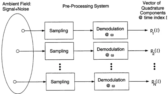
The receiving array and the associated data acquisition system are responsible for tem-poral and spatial sampling of the ambient wave field. Vertical deployment, as shown in Figure 2-1, is common for mode resolving arrays. Figure 2-2 shows a typical data acqui-sition and pre-processing system. Standard pre-processing of the antenna outputs consists of temporal sampling followed by demodulation at the frequency of the source. The re-sult is a vector time series, p(l), of quadrature components representing the pressure field.

Most processors include filters to improve input signal-to-noise ratio. The rest of this thesis implicitly assumes that these basic pre-processing steps have been taken.

Ambient Field:

Signal+Noise Pre-Processing System

Vector of Quadrature ("_mnrnnantfc te index I P ₁(t) P2(1) PN( )

Figure 2-2: Data acquisition and pre-processing

The ocean model used in this research consists of a horizontally-stratified medium with arbitrary sound speed and density profiles in the vertical which is bounded from above and below by semi-infinite halfspaces. The upper halfspace above the water's surface is modeled as a vacuum, and the lower halfspace has characteristics similar to the sediment layers. Range dependencies may be incorporated into the model by propagating signals through a cascade of range-independent sections.

2.2

Normal Mode Representation of Narrowband Signals

The acoustic wave equation, with parameters and boundary conditions derived from the environment, describes the propagation of sound in a horizontally-stratified waveguide. The sound pressure field generated by a narrowband source is conveniently characterized by Fourier transforming the wave equation to obtain the Helmholtz equation. Normal mode solutions to the Helmholtz equation are the focus of this section. The frequency dependence

2.2.1

Modal Propagation in a Range-Independent Waveguide

In this section the environment is assumed to be range-independent and is characterized by the sound speed profile c(z) and the density profile p(z) which vary with depth. Let p(r, z) be the sound pressure for a narrowband source and the Helmholtz equation becomes

2

~~~~~2

(z) = c2z

(21

rd-

rd

dp

₌

_k

r dr \dr/ pWzaz '' c2 z

where k is the wavenumber associated with the medium. F(r, z) is the forcing function asso-ciated with the acoustic point source. Consider the idealized range-independent waveguide shown in Figure 2-3. The waveguide is of depth H with a pressure release boundary at the surface (z = 0) and a perfectly rigid boundary at the bottom (z = H). An arbitrary depth-dependent sound speed profile is assumed. The rigid (non-propagating) bottom boundary condition simplifies this initial development; a brief discussion of the implications of more realistic bottom conditions follows.

Sound Speed r=O r

_- m,

z=O

z=H

w

Pressure Release Surface (p=O)

Rigid Bottom (P= O)

i , , , , , , > ,~~d

7/////////////

z Z

Figure 2-3: Idealized range-independent waveguide

The separation of variables technique yields solutions to the unforced (F = 0) Helmholtz equation of the form [10]

p(r, z) = H(1)(kmr)qOm(z) (2.2)

the first kind. The depth function qbm satisfies the following eigenvalue problem

d2tbmr

dz0 2 + [k 2_{(z) -k]m = 0 (2.3)}

dz2 qk(z

For the simple boundary conditions described above, this equation is a classical

Sturm-Liouville problem where the depth functions (modes) form a complete orthonormal (CON)

set. Thus, the solution to Equation 2.1 for a point source consists of a weighted sum of the

normal modes

p(r,z) = wmH(l)(kmr),m (z).

(2.4)

m

When the forcing function F is known, the orthogonality of the modes may be exploited to

determine the weights, win. In the case of a unit-normalized point source at depth zs and

range r = 0, the pressure at depth z and range r becomes

-i~r/4 eikmr

p(r, z) = e 4

E'

Z

p(zs) V87rr m

An asymptotic approximation for the Hankel function has been used to derive this result.

As shown in Equation 2.5 the source excites each mode at a level proportional to the value

of the mode function

Ok

at the source depth z.

While the sum is infinite, only a finite

number of modes actually propagate in the waveguide. Higher than a certain mode number

m, the horizontal wavenumbers are imaginary, therefore contributions from these modes

are exponentially decaying with range. Modes with imaginary km are called evanescent and

do not affect the modal sum if the point of interest is at any significant distance from the

source.

Although the essential features of the normal mode decomposition are revealed in the

idealized waveguide example, practical models require more realistic bottom conditions.

Jensen et. al. [12] provide a clear generalized derivation which incorporates arbitrary bottom

boundary conditions. The additional mathematical rigor offers few new insights, however.

Suffice it to say that at long ranges away from the source, the signal may always be written

as a weighted sum of the propagating modes.

Consider the following example of a realistic waveguide. This simulation environment

is used for all of the numerical examples in the later chapters.

Deep Water Simulation Environment

The channel is 4000 meters deep and is characterized by a Munk profile [13]. This profile is a canonical deep water sound speed profile with a single minimum. In this case the min-imum sound speed is 1480 m/s at an axis depth of 1000 meters. Water density is assumed to be 1.0 g/cm3. The left side of Figure 2-4 shows the sound speed profile for the simulation environment. A 70 Hz narrowband source is used for all the numerical examples. The right

Profile Modeshapes (70 Hz) U -1000 E c -2000 0 -3000 -Annn 1480 1500 0 2 4 6 8 10 12 14 16 (m/s) Mode Number

Figure 2-4: Sound speed profile and modeshapes for the deep water waveguide

side of Figure 2-4 is a plot of the modeshapes for the first 16 modes associated with the source. Note that the vertical extent of these modes effectively defines a channel in which low-angle rays can propagate outward from a source on the axis. The modeshapes were computed using a normal mode code developed by Baggeroer [14].

Consider sampling the wave field generated by a point source using a receiving array. Assuming that the field is composed of a subset of M discrete modes, the sum in Equa-tion 2.5 is most conveniently written using linear algebra notaEqua-tion. The vector of pressures measured by an N-element vertical array is defined as follows

p = bEPx (2.6)

where

in the signal processing,

{ Ibj2 = 2

*~~~ j f b

* E is an N x M matrix of sampled modeshapes,

01

* P is an M x M diagonal propagation matrix,

0

eikmr

0

0

0

* x is a vector of mode depth amplitudes containing the source excitation,

1

(Zs)

02 (Zs)

OM(Zs)

Equation 2.6 provides a compact representation of modal propagation in a range-independent waveguide. The matrix P transforms the initial excitation of the modes at the source (rep-resented by x) to the excitation levels at the receiver. The diagonal structure of the propa-gation matrix P reflects the fact that there is no transfer of energy among the modes. Note that the matrix E requires a slight modification to account for phase difference across the array if all sensors are not at the same range, i.e., if the array is tilted. The inclusion of

b in the model implies that the received pressures are contained in a zero-mean Gaussian

random vector. (2.7) (2.8) (2.10) P = Z e-i7r/4 0 p (z,,) -\/-8-7r 0

2.2.2

Modal Propagation in a Range-Dependent Waveguide

As previously indicated, models of range-dependent channels typically consist of a cascade of range-independent sections. A partial separation of variables solution leads to a set of mode depth functions and horizontal wavenumbers for each section. Regardless of the range-dependence of the waveguide, the signal at a receiving array may be written as a weighted sum of the "local" modes, i.e.,

p = bEPx

where E is a matrix of sampled modeshapes for the segment containing the receiver. As defined in Section 2.2.1, and x represent the inherent phase uncertainty and the initial modal excitation, respectively. Modifications to the matrix P account for the range depen-dent nature of the propagation.

In general, range dependencies in a channel lead to transfers of energy among the modes. As a result of this coupling, P is no longer a diagonal matrix. Full coupled mode theory usually requires numerical solution of the range equations for each segment in order to obtain the coupling parameters.

For mildly range-dependent environments, however, the adiabatic approximation leads to an analytically-tractable range solution. Adiabatic normal mode theory assumes that the range dependence is gradual enough that an individual propagating mode adapts with range but does not transfer energy into the other modes. In other words, the modeshapes and wavenumbers vary with range, but the modes do not couple or scatter into each other. The adiabatic approach results in the following summation for the pressure at a single receiver

i e -i~r/4

e

p(r, z) = e (Z)O(Z) k m (2.11)

p(zs>v/8r m s krn-mr

where the range-averaged wavenumber is defined as

km = 1 km(r')dr', (2.12)

and /bm(z) and q3ra(Z) represent the modeshapes at the source and receiver locations,

For an adiabatic model, the P matrix is the same as in Equation 2.9 provided that the range-averaged wavenumber km is substituted for km.

2.2.3

Modal Propagation in a Random Waveguide

The models discussed in the previous sections assume that the ocean is a deterministic medium, however experimental evidence indicates the presence of internal wave fields which can perturb the local sound speed profile. These perturbations introduce fluctuations in acoustic signals which can be simulated using stochastic propagation models. The literature contains many references to wave propagation in random media. In particular, Dozier and Tappert have presented a statistical theory of modal propagation in a random ocean [15, 16]. Baggeroer and Kuperman propose a paradigm for matched field processing in a stochastic

channel [17].

The framework of Equation 2.6 still applies for a random ocean, provided that the definitions of b and P are modified accordingly. The propagation term P becomes a matrix of zero-mean Gaussian random variables. The zero-mean and Gaussian assumptions again reflect the phase uncertainty inherent in the signal processing. The source scaling term, b, is a constant that is retained for consistency with the models described in the two previous sections (b[2 = a2). For the random case a channel is specified in terms of the second order statistics of the modal excitation, i.e., £ {PxxtPt}.

Baggeroer and Kuperman offer several examples of random channels [17]. The one that is relevant for later examples in this thesis corresponds to an adiabatic channel with internal waves. For this channel the second order statistics are shown below

£ {PxxtPt}

(1 - 'y)diag [xoxt] + xoxt

where

O < y < 1.

(2.13)

The operator diag indicates that only the diagonal terms are used; the off-diagonals are set to zero. The vector x represents the modal amplitude at the receiver for a deterministic adiabatic channel. Coherence of the signal is determined by the parameter -y. When y is equal to 1, the modes are phase locked; the propagation characteristics correspond to those of a deterministic adiabatic channel. At the other extreme, when -y is equal to 0, the modes are phase random; this implies a totally incoherent signal. The structure in Equation 2.13 ensures that there is no energy exchanged among the modes, hence the adiabatic assumption

is satisfied.

2.3

Problem Formulation

As indicated in Chapter 1, the average power in the normal modes provides valuable in-formation about the propagation environment. The objective of the algorithms discussed in this thesis is to estimate the power in each mode given a set of pressure measurements from an array of sensors. Since high order modes are less energetic at long ranges and can be resolved temporally, subsequent discussions focus on estimating the power spectrum of the low order modes.

Regardless of the characteristics of the waveguide, the signal measured by a receiver may be written as a weighted sum of the local modes

p = Ea (2.14)

where E is a matrix of local modeshapes and a is a vector of coefficients associated with the modes. The vector a contains the relative levels of each mode, as determined by the

initial source excitation and the propagation characteristics of the medium, i.e.,

a = Px. (2.15)

From the definitions of b, P, and x used in each of the previous sections, a is a zero-mean, Gaussian random vector with the M x M correlation matrix SM defined below,

SM = {aat} = £

{

u

f {pxxtPt}

(2.16)

The diagonal terms of SM are the average powers in the modes and the off-diagonal terms indicate correlation among the modes. Clearly the propagation environment, represented by P, determines the structure of the mode correlation matrix. In general SM is an arbitrary positive semi-definite M x M matrix, but two special cases are worth mentioning.

Coherent Modes

do not occur independently of phase variations for any other mode. Deterministic, time-invariant channels are always coherent; random or time-varying channels may or may not be coherent depending on the statistics of the propagation matrix P. Most matched field processing (MFP) algorithms rely on coherent signal models to generate replica vectors. Coherency is a reasonable assumption for transmission over moderate distances within an ocean basin. For example, Polcari has shown that the Arctic Ocean is a stable, highly

coherent channel [9].

When the modes are perfectly correlated, the SM matrix has rank 1 (only one non-zero eigenvalue). As a result, two parameters completely specify the correlation structure, i.e.,

=

PT

[aTafl.

PT

Incoherent Modes

A signal is totally incoherent when the modes are phase random with respect to one an-other. For example, data taken with one of the HIFT vertical line arrays indicates that a signal which was transmitted over an 18,000 km path consisted of an incoherent sum of modes [6]. Phase coherence of the normal modes is an aspect of global propation that is not well-understood. Signal randomization is more often considered in the context of rays. Theory predicts that signals traveling along different ray paths are uncorrelated at long ranges. Brekhovskikh and Lysanov [10] provide a useful discussion of this topic.

Incoherent modes are uncorrelated, thus SM is a diagonal matrix,

2(a2) 0 ... 0

SM = 0

(a2)

0

: .

"

,

0

0 ... 0 9(a)

rank M.

The goal of this thesis is to investigate new methods for estimating the modal power distribution from sound pressure measurements made with a vertical line array. In a realistic ocean environment, the measured pressure consists of the modal signal plus noise

p = Ea+ n. (2.19)

The signal and the noise are independent vector random processes, therefore a statistical description of the received field is useful. The modal signal is a zero-mean process with covarinace

Ss = E {EaatEt} = ESMEt. (2.20)

Ambient noise in the waveguide is assumed to be zero-mean with covariance SN. The structure of SN is discussed in Section 2.4.1. The above assumptions imply that p is a zero-mean random vector with the covariance given below

S = SS + SN. (2.21)

S is an N x N matrix referred to as the sensor covariance matrix. The algorithms described in the remaining chapters attempt to extract the average modal powers (diagonal terms of SM) from the pressure field characterized by S. In the case of a partially incoherent or random channel, the off-diagonal of SM terms contain valuable information, but a thorough study of their estimation is beyond the scope of this thesis.

2.4

Important Considerations in Modal Array Processing

The purpose of this section is to highlight important signal processing issues that arise in us-ing vertical line arrays to sample modal fields. Later chapters characterize the performance of estimators in terms of the four criteria discussed below.

2.4.1

Ambient Noise

Ambient noise in the waveguide is described by SN, the noise covariance among the array elements at a specific frequency. Ocean noise can be divided into three general categories:

1. Sensor noise: Spatially-correlated noise with the covariance matrix Sw =

c2, I

2. Distributed noise: Correlated noise with the covariance matrix Sc whose structure is determined by the propagation environment. One example of distributed noise is surface-generated noise.

3. Discrete noise sources: Noise sources that have signal-like qualities and contribute to the far-field effects that are described by the discrete modes. The covariance of discrete noise is denoted by

SD = EddtEt (2.22)

where d is the vector of mode amplitudes for the discrete noise source. The total noise covariance is

SN = SW + SC + SD (2.23)

Since the propagation environment is inhomogeneous in the vertical, the signal-to-noise ratio (SNR) differs from sensor to sensor on the array. It is sometimes convenient to define the SNR at the input to an N-element array as the geometric mean of the SNR's at each array element i.e.,

SNR = [(SNR

)(SNR

)... (SNRN)]k

or in dB

1 N

SNR=

H

10 log

(2.25)

n=1

In a homogeneous environment where the SNR is identical at all elements, the above equa-tion reduces to

SNR

Chapter 1 notes the prevalence of low SNR environments in global propagation studies. For example, input SNR's (before pre-processing) for the HIFT Monterey vertical line array were approximately -10 to -15 dB on a single hydrophone [18]. Since low SNR's can adversely

affect performance, it is important to consider the impact of noise on mode estimation algorithms.

2.4.2 Modal Orthogonality

The second major issue in modal estimation concerns the array's ability to sample the pressure field. In principle, a filled array which spans the water column can resolve a complete set of orthonormal modes. In practice however, arrays consist of discrete elements spanning a limited aperture. As a result, the sampled mode shapes may not be orthogonal, even though the true modes form a CON set. Realistically, an array can spatially resolve only that finite set of modes which are adequately sampled by its sensors.

One way of measuring the orthogonality of the sampled modes is to examine the mode-shape correlation matrix EtE. If the sampled modes are orthogonal, this matrix is diagonal. (For the purpose of this thesis, it is convenient to assume that the modeshapes are scaled equally such that orthogonal modes correspond to an EIE matrix that is a mulitple of the identity matrix. This assumption simplifies bookeeping somewhat, but is not a necessary condition for orthogonality.) If the sampled modes are not orthogonal, the matrix contains non-zero off-diagonal terms which represent the "cross-talk" between the modes. As an example, consider sampling the deep water environment with an array. The array geometry described below is used for numerical examples in the rest of the thesis.

Simulation Array

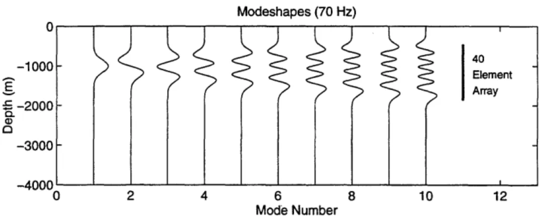
The array consists of 40 elements with 35 meter sensor spacing and spans almost 1400 meters. Figure 2-5 shows the first 10 modeshapes in relation to the position of the array. The top sensor is located at a depth of 475m, resulting in 40 percent of the elements being positioned above the channel axis. The array is designed to adequately sample the first 10 modes.

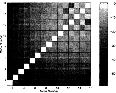
Figure 2-6 is a plot of the modeshape correlation using the first 16 modes of the wave-guide for the 70 Hz frequency band. The plot shows the elements of the correlation matrix on a log scale (10 log1 0EtE), normalized such that the maximum element corresponds to

0 dB. Note that above mode 11, the off-diagonal terms become significant. This is expected since the array is designed to sample the lowest 10 modes.

Modeshapes (70 Hz) U -1000 a -2000 a) 0 -3000 -Annn 0 2 4 6 8 10 12 Mode Number

Figure 2-5: Simulation array for the deep water waveguide

modeshape correlation matrix, defined as

DOFeff

(t4

i)(2.27)

where the

,U

i.e., when only one mode is included in E. For M > 1, the effective degrees of freedom

is a measure of how many linearly independent vectors are contained in E. If the modes are orthogonal, then the number of effective degrees of freedom is approximately equal to

M. As the modes lose orthogonality, DOFeff decreases. The plot in Figure 2-7 shows the

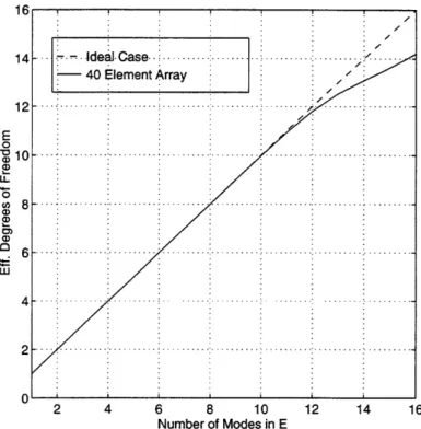
effective degrees of freedom vs. number of modes included in E. The dashed line corresponds to DOFeff for an ideal filled array that completely spans the water column. The solid line represents the degrees of freedom for the simulation array. Based on the figure, the array samples at least the first 11 modes adequately, but begins to lose degrees of freedom when 12 or more modes are included. Note that DOFeff is a useful measure of orthogonality for the lowest order modes. Due to aliasing, if only a subset of higher order modes are included in E, then the degrees of freedom measurement might be misleading.

The location of the array and the spacing of the sensors determines the orthogonality of the sampled modeshapes. The number of modes which can be accurately estimated by an array is limited by the orthogonality, but is also influenced by the estimation method. Determining the number of modes to estimate is usually an ad hoc procedure. Analysis of estimation algorithms must address this issue.

it 14 12I' .Q E z 8 0 E

Fa7

Figure 2-6: Modeshape correlation for the deep water waveguide

2.4.3

Estimation of the Covariance Matrix

Many mode estimation algorithms require the sensor covariance matrix S which contains the second order statistics of the sound field. In practice this matrix must be estimated from the vector time series of pressure measurements taken by the array. The sample covariance is defined as the average of outer products of the data snapshots,

l t

S : = L

pip-

iE

(2.28)

i=1

If the field is zero-mean, then S is an unbiased estimate of the true covariance. In addition, if the field is Gaussian (e.g., the model defined in Section 2.3), then Equation 2.28 generates a maximum likelihood estimate of the covariance [19]. The statistics of the sensor covariance estimate are important, especially for adaptive array processing. Goodman has shown that the sample covariance follows a complex Wishart distribution of order N with L degrees of freedom, where N is the number of sensors and L is the number of data snapshots [20]. Many multivariate statistics textbooks, such as the one by Muirhead [21], discuss the Wishart distribution and its relation to the sample covariance. Steinhardt [19] provides an excellent review of the subject with a focus on array processing applications. The properties of

16 _{! !} .

_~/.

~~/

~ ~ ~

4

Figure 2-7: Degrees of freedom for the simulation array

the complex Wishart distribution can be used to derive analytical results concerning the statistics of estimates. For example, Capon and Goodman have demonstrated that using a finite number of snapshots in the average leads to bias in algorithms which require the inverse of the sample covariance matrix [22]. Many adaptive algorithms are affected by the number of snapshots used to estimate the covariance. The analysis in the later chapters evaluates the performance of estimators with respect to the number of data snapshots available.

2.4.4 Signal Coherence

Signal coherence is another major issue to consider. As discussed in Section 2.3, coherent

modes lead to a rank one signal covariance matrix Ss. As coherence is lost, the rank of Ss increases. Many adaptive algorithms, e.g., those used in matched field processing, exploit the coherence of signals in order to accurately estimate the desired parameters. Since mode coherence is not guaranteed at long ranges, it is important to analyze the effects of coherence on modal estimation strategies.

2.4.5

Performance Measures

This section defines several empirical measures of performance which are useful in analyzing the issues presented in the preceding sections. Since the thesis is primarily concerned with estimating the average powers in the modes, an error vector is defined as follows

e = diag { SM-SM|}

.

A hat distinguishes the estimated mode correlation from its true value. The diag operator indicates that the vector consists of the diagonal elements of the error matrix.

Mode estimates are random variables, thus the error statistics are useful performance measures. The expected error or bias indicates how close the estimates are to the actual parameters on average. Error variance provides a measure of the spread of an estimate around its mean. Note that the error variance is equal to the variance of the estimate. Low variance is a desirable characteristic for an estimator. The Cramer-Rao bound provides a useful lower bound on the variance of an unbiased estimate [23]. Derivation of this limit requires only a knowledge of the conditional probability density of the observations given the true parameters. The bound on the variance of the average power estimates is expressed in terms of the elements of the Fisher information matrix J, e.g., for the ith mode power estimate

var {[§M]iij}

> [J']ii.

The Fisher information matrix for the mode power estimation problem is derived in Ap-pendix A. Therrien notes that a correction to the bound is available for the case of a biased estimator [23]. The correction term involves the gradient of the bias with respect to the desired parameter vector. Thus, the correction is unnecessary if the bias is due to noise which is independent of the modal signal.

Sometimes a scalar measure of the error is useful. The total error is defined as the trace of the error matrix, i.e.,

2.5

Summary

This chapter has presented a general mathematical model for mode propagation in an ocean waveguide. Both deterministic and random channels fit into the same framework, provided that the propagation parameters are specified appropriately. Section 2.3 has defined the acoustic mode estimation problem in an array processing context. The final section has outlined important issues which will be used in the performance analysis of the estimators developed in the following chapters. In addition this chapter has described a deep water environment and an array geometry for numerical simulations.

Chapter 3

Least Squares Methods

The previous two chapters have motivated and defined the modal estimation problem. In particular, Chapter 2 developed the necessary background and stressed the importance of different aspects of the signal processing. The purpose of this chapter is to review standard methods for estimating the modal powers.

In theory the orthogonality of the normal modes permits the use of spatial matched fil-ters. For example, Ferris [24] determines the weight associated with each mode by "match-ing" the received signal to the sampled modeshape. This method relies on the orthogonality of the sampled modeshapes, which is not always a valid assumption in practice. Recall from Chapter 2 that the orthogonality of the modes depends on the sensor spacing and position of the array. Since logistics and funding often limit the number of sensors that can be deployed, the desired modes are not always orthogonal. If the sampled modeshapes are not orthogonal, power from one mode can leak into estimates of the adjacent modes. Conven-tional approaches often apply Least Squares (LS) estimation theory to reduce the effects of non-orthogonal modeshapes. LS techniques compute a set of weights which minimize the total squared error between the measured and estimated modal fields.

Many researchers have addressed the problem of estimating the modes in an acoustic signal. Clay was the first to recognize the important link between the modal decomposition and array processing [25]. Hinich developed a maximum likelihood method for depth local-ization using the normal modes [26]. Since that time, a class of matched field processing algorithms based on normal mode theory has been developed. A survey of the current lit-erature indicates that Matched Mode Processing (MMP) applications generate most of the

mode estimation research [2, 3, 4, 27]. All of the standard estimation techniques used for MMP are based on minimizing a squared error criterion. A review article by Voronovich et.

al. compares five modal estimators using numerical simulations and experimental data [8].

Two recent theses have addressed the modal estimation problem. Polcari provides a thor-ough overview of conventional modal beamforming, including a practical application to a coherent Arctic channel [9]. Sperry discusses the use of least squares modal filtering in the context of a long-range propagation experiment [28].

This chapter is organized as follows. Section 3.1 develops the standard least squares estimator and analyzes it using a few numerical examples. The performance evaluation ad-dresses the main issues outlined in Chapter 2: ambient noise, mode orthogonality, estimated covariances, and signal coherence. Finally, Section 3.2 summarizes the characteristics of the LS estimator, thereby motivating the search for a new approach.

3.1

Standard Least Squares

Standard modal estimation algorithms produce time series using a least squares approach to generate the mode amplitudes for each data snaphsot. For a single pressure vector p, the LS technique minimizes a squared error criterion in order to estimate the mode amplitudes, i.e.,

alsi = min Ip - Eaj2. (3.1)

This method implicitly assumes that the received pressure consists only of the modal sig-nal Ea and ignores the noise components. The minimization problem stated above has a well-known solution [29, 30, 31],

i= (EtE)-lEtp. (3.2)

Consider the case where the received pressure consists of the modal signal only. It is trivial to show that ais is equal to the true mode amplitudes, provided that (EtE)-1 exists and the number of modes in the estimate is greater than the number of modes in the signal. Now suppose that additive noise corrupts the pressure measurements. The linearity of the LS processor implies that the noise corrupts the resulting mode estimates as well. For least squares methods to be effective, the SNR must be high enough so that the signal

components dominate the noise.

Note that if the modes are orthogonal then (EtE)- 1is a multiple of the identity matrix, and the least squares solution corresponds to Ferris' matched filtering approach. If the modes are not orthogonal, then the inverse in Equation 3.2 is usually computed using the Singular Value Decomposition (SVD).

Recall that the desired parameters to estimate are the average powers in the modes, i.e., the diagonal terms of the modal correlation matrix. Polcari [9] suggests that the second order modal statistics, can be obtained from the time series as an average of outer products

1

ala

SMLS = L a (3.3)

i=1

where L is the number of data snapshots available. Since the least squares processor is linear, Equation 3.3 is obviously equivalent to

SMLS = (EtE)-Et

{

(3.4)

where S is the estimated sensor covariance matrix.

The following example illustrates the basic characteristics of the least squares estimator. Subsequent sections examine specific aspects of the estimator's performance in more detail.

Deep Water Example

The simulation environment is the deep water waveguide described in Chapter 2. Figure 2-4 shows the modeshapes for the 70 Hz narrowband source used in the following examples. It is convenient to define a standard test signal for use throughout the thesis. The signal consists of a coherent sum of the lowest 8 modes: the odd modes (1, 3, 5, 7) are excited at a reference level of 0 dB and the even modes (2, 4, 6, 8) are excited at -10 dB. Modes 9 and higher are not present in the signal.' Additive noise in the environment consists of white sensor noise only. The power level of the white noise controls the effective signal-to-noise ratio for each example. As defined in Section 2.4.1, the input SNR is the geometric mean of the SNR's at each sensor in the array. The 40-element simulation array, described in

'Parameters of the test signal are somewhat arbitrary. The alternating pattern in the first 8 modes is for visualization purposes. The absence of modes 9 and higher is useful in determining how well the processing handles nulls in the modal power spectrum.

Section 2.4.2, samples the water column. Least squares processing attempts to resolve the power in the first 10 modes of the waveguide.

First consider the case where the sensor covariance is known exactly and does not have to be estimated from snapshot data. While this is clearly not a practical assumption, the ideal covariance case indicates the best possible performance of the estimator. Figure 3-1 shows the ideal LS estimates of the power in the first 10 modes for three different signal-to-noise ratios: 10 dB, 0 dB, and -10 dB. Circles denote the true power distribution and

SNR: 10.0 dB , .' , i ! i f I \ \ / \ \ 3 \ \ / \ \ / \ I/ \

\

Figure 3-1: Least squares power estimates for the deep water example

asterisks represent the LS mode estimates. The dashed line which interpolates the LS results is for viewing purposes; the estimate only exists for integer mode numbers. The top plot

o TRUE LS - -5 --10 -15 0. -20 -25 - ₀-5 a3- S-10--15 0 0,.--20 -25 -30 -5 -5 B -15 0 -20 -25 N * '.s, 7 , \ " , /,,, , " 0 0 0N 0 " 0 0 0 O0 .. I , -- -'; o TRUE LS 1 2 3 4 o TRUE LS 7 8 9 10 __ T i i . i . i i .i f I I I I I I I