HAL Id: hal-02326729
https://hal.archives-ouvertes.fr/hal-02326729
Submitted on 22 Oct 2019
HAL is a multi-disciplinary open access
archive for the deposit and dissemination of sci-entific research documents, whether they are pub-lished or not. The documents may come from teaching and research institutions in France or abroad, or from public or private research centers.
L’archive ouverte pluridisciplinaire HAL, est destinée au dépôt et à la diffusion de documents scientifiques de niveau recherche, publiés ou non, émanant des établissements d’enseignement et de recherche français ou étrangers, des laboratoires publics ou privés.
Heritability estimates from genomewide relatedness
matrices in wild populations: Application to a passerine,
using a small sample size
C. Perrier, B. Delahaie, A. Charmantier
To cite this version:
C. Perrier, B. Delahaie, A. Charmantier. Heritability estimates from genomewide relatedness matri-ces in wild populations: Application to a passerine, using a small sample size. Molecular Ecology Resources, Wiley/Blackwell, 2018, 18 (4), pp.838-853. �10.1111/1755-0998.12886�. �hal-02326729�
Heritability estimates from genome wide relatedness matrices in wild populations:
1
application to a passerine, using a small sample size
2 3
Running head: GRM in Corsican blue tits
4 5
Perrier C*, Delahaie B, Charmantier A.
6 7
Centre d'Ecologie Fonctionnelle et Evolutive, CNRS-UMR5175 CEFE, Montpellier,
8
France
9 10
*corresponding author: charles.perrier@cefe.cnrs.fr
11 12
Molecular Ecology Resources - Special issue Association Mapping in Natural
13
Populations.
14 15
Keywords: heritability; genetic correlation; RAD-sequencing; GRM; pedigree;
16
partitioning; phenotype; blue tit; SNP; Cyanistes caeruleus
17 18
Abstract
19
Genomic developments have empowered the investigation of heritability in wild
20
populations directly from genome wide relatedness matrices (GRM). Such GRM based
21
approaches can in particular be used to improve or substitute approaches based on
22
social pedigree (PED-social). However, measuring heritability from GRM in the wild has
23
not been widely applied yet, especially using small samples and in non-model species.
24
Here, we estimated heritability for four quantitative traits (tarsus length, wing length, bill
25
length and body mass), using PED-social, a pedigree corrected by genetic data
(PED-26
corrected) and a GRM from a small sample (n = 494) of blue tits from natural
27
populations in Corsica genotyped at nearly 50,000 filtered SNPs derived from RAD-seq.
28
We also measured genetic correlations among traits and we performed chromosome
29
partitioning. Heritability estimates were slightly higher when using GRM compared to
30
PED-social, and PED-corrected yielded intermediate values, suggesting a minor
31
underestimation of heritability in PED-social due to incorrect pedigree links, including
32
extra-pair paternity, and to lower information content than the GRM. Genetic correlations
33
among traits were similar between PED-social and GRM but credible intervals were very
34
large in both cases, suggesting a lack of power for this small dataset. Although a
35
positive linear relationship was found between the number of genes per chromosome
36
and the chromosome heritability for tarsus length, chromosome partitioning similarly
37
showed a lack of power for the three other traits. We discuss the usefulness and
38
limitations of the quantitative genetic inferences based on genomic data in small
39
samples from wild populations.
Introduction
41
Estimating additive genetic variance and heritability of quantitative traits is a major aim in
42
evolutionary biology because they are crucial components of all evolutionary models.
43
Further, fine-scale dissection of the genomic basis of quantitative traits in the wild, using
44
methods such as genome wide association and linkage mapping, requires validation
45
that the traits being mapped are actually heritable. New sequencing technologies have
46
empowered the estimation of genomic relatedness matrices (GRM) between individuals
47
(Visscher et al. 2008; Huisman 2017; Gienapp et al. 2017), feasibly without any social
48
pedigree (PED-social) recorded in the field. Since in a quantitative framework, common
49
SNPs additively explain a large part of genetic additive variance, it is possible to use
50
such realized relatedness estimated from genomic data to measure traits’ heritability in
51
wild populations (Yang et al. 2010). Furthermore, by aligning markers against a
52
reference genome, heritability can then be partitioned among chromosomes (or at other
53
genomic scales) enabling testing quantitative models of increasing heritability with the
54
number of genes per chromosomes (Yang et al. 2011b), or alternatively, identifying
55
chromosomes displaying higher genetic variance than expected. GRM estimates and
56
chromosome partitioning, first applied on human data (Yang et al. 2010; 2011b), were
57
then applied in well-known free-ranging animal populations (Great tits, Parus major,
58
Robinson et al. 2013; Soay sheep, Ovis aries, Bérénos et al. 2015) for which thousands
59
of individuals were genotyped at thousands of loci. There have been fewer empirical
60
applications of these methods to smaller samples (but see Wenzel et al. 2015; Silva et
61
al. 2017), although they have great potential in the current context of genomic tools
being increasingly applied to natural populations (Gienapp et al. 2017) that often rely on
63
relatively small samples.
64
Three important limitations for estimating GRM and GRM based heritability are
65
the number of SNPs, the number of individuals and the sampling variance (Visscher &
66
Goddard 2015). The limitation from the number (as well as diversity and quality) of
67
markers and their ability to resolve relatedness essentially vanished when we entered
68
the genomic era (Csillery 2006; Stanton-Geddes et al. 2013; Gienapp et al. 2017). The
69
sample size of individuals genotyped and phenotyped, however, remains an issue. For a
70
given dataset, the number of individuals included will influence both error and median
71
values of heritability estimates, as tested in two studies (Stanton-Geddes et al. 2013;
72
Visscher & Goddard 2015). Nevertheless, reasonable heritability estimates can be
73
reached using 150 to 200 individuals, as showed in a study on barrelclover (Medicago
74
trunculata, Stanton-Geddes et al. 2013). However, different species, demographic
75
contexts, and sampling strategies will likely perform differently for a similar number of
76
individuals, number of markers and traits’ architecture. Visscher & Goddard (2015)
77
showed that for designs that use genetic markers to estimate relatedness among
78
randomly sampled individuals from a population (which may be a common situation for
79
non-model species in natural populations), the error in heritability estimation is inversely
80
proportional to the squared sample size and is proportional to the effective population
81
size. Therefore, heritability estimates based from genetic marker relatedness in
82
extremely large populations will likely require thousands of samples (e.g. marine pelagic
83
fish (Gagnaire & Gaggiotti 2016)), but also thousands of loci (given the small linkage
84
disequilibrium among loci). Nevertheless, for populations of smaller size, a sampling
strategy aiming at capturing variance in realized relatedness offers possibilities to obtain
86
robust heritability estimates bounded by reasonable standard errors.
87
While genomics offers promising potential to obtain quantitative genetic
88
parameters for virtually any species or population (Gienapp et al. 2017), it has only been
89
used in a few studies to-date and more applications in smaller samples and non-model
90
species are needed. The first studies to estimate genomic heritability and partition
91
variation across the genome elsewhere than in humans were, understandably, focusing
92
on already well-known populations and species. In particular, analysis of 2644
93
individuals at 7203 SNPs from a long term population study of great tits was the first
94
application of quantitative genomics to a wild population (Robinson et al. 2013). The
95
Soay sheep (Ovis aries) also benefited from such a genomic quantitative genetic study,
96
with 5805 individuals genotyped at 37,037 autosomal SNPs (Bérénos et al. 2014). This
97
study revealed that most of the additive genetic (co)variances in sheep body size traits
98
were captured by half of the SNPs. These pioneering studies enabled the verification of
99
the power of quantitative genomics on known populations with long-term pedigrees and
100
characterized quantitative genetic parameters (Edwards 2013). Other authors also
101
estimated heritability from GRM in datasets with much less individuals, e.g. 200
102
barrelclover (Medicago trunculata) individuals genotyped at more than 5 million SNPs.
103
Wenzel et al. (2015) estimated genome-wide heritability in 695 red grouse (Lagopus
104
lagopus scotica) genotyped at 384 SNPs. Silva et al. (2017) estimated quantitative
105
genomic parameters in 1,898 house sparrows (Passer domesticus) genotyped at 6,348
106
SNPs and in 825 collared flycatchers (Ficedula albicolis) genotyped at 38,689 SNPs.
107
These examples confirmed the usefulness of the method in new cases and with fewer
individuals. Although we did not perform a thorough meta-analysis, there was a trend
109
among these studies for an increase, among and within studies, of heritability estimates’
110
standard errors with decreasing sample size and SNP amount. Nevertheless, and
111
surprisingly considering the number of studies performing genomic analyses since the
112
beginning of the genomic era, there are relatively few applications of genomic data to
113
estimate heritability, genetic correlations and chromosome partitioning, using smaller
114
datasets.
115
Here, we assessed heritability, genetic correlations, and chromosome partitioning
116
for four phenotypic traits, namely tarsus length, wing length, bill length, and body mass,
117
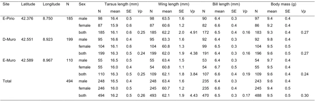
in a collection of 494 individuals of Corsican blue tits (Cyanistes caeruleus ogliastrae)
118
from three closely located sites in Corsica (Figure 1). Based on mitochondrial genetic
119
and phenotypic data, blue tits in Corsica and Sardinia have been qualified as a
120
subspecies, Cyanistes caeruleus ogliastrae (Kvist et al. 2004). The focal populations are
121
ideal for quantitative genetic study because of the availability of pedigree, phenotypic
122
and genetic data gathered through a long-term study (Charmantier et al. 2016). Based
123
on microsatellite and SNP genetic data, important gene flow together with significantly
124
low genetic differentiation have been suggested between Corsican populations (Porlier
125
et al. 2012; Szulkin et al. 2016). Phenotypic variance for the four aforementioned traits
126
has been characterized as quantitative and moderately to highly heritable (Charmantier
127
et al. 2004b; Blondel et al. 2006; Charmantier et al. 2016). The latest published results
128
based on 17 to 27 years of monitoring, provided population-specific significant
129
heritability ranging from 0.43 to 0.57 for tarsus length, 0.20-0.33 for wing length,
0.18-130
0.34 for bill length, and 0.22-0.32 for body mass. All trait combinations showed
significant additive genetic covariance (COVA) in at least one population; in particular
132
COVAs between wing length and tarsus length and between wing length and body mass
133
were significantly positive (Delahaie et al 2017). Lastly, from 18 to 25% of young have
134
been identified as extra-pair offspring in these Corsican blue tit populations (Charmantier
135
et al. 2004a), which may lead to slight underestimation of trait heritability from a
field-136
based social pedigree (Charmantier & Réale 2005).
137
The general objective of this study was to test the effectiveness of GRM to
138
estimate heritability and genetic correlations among traits and to perform heritability
139
partitioning while using a relatively small sample size of Corsican blue tits. We produced
140
a dataset of 494 Corsican blue tits, from three sites (sample sizes of 110, 185 and 199),
141
genotyped at nearly 50,000 filtered SNPs derived from RAD-seq and phenotyped for
142
four quantitative phenotypic traits (tarsus length, wing length, bill length, and body
143
mass). We looked for erroneous links in the social pedigree (PED-social) using the
144
genetic data, in order to build a corrected social pedigree (PED-corrected). We
145
estimated heritability using both GCTA (Yang et al. 2011a) and MCMCglmm (Hadfield
146
2010) for the 494 genotyped individuals (with the three sites pooled or separately),
147
based on GRM, social and corrected. Heritability differences between
PED-148
corrected and PED-social were computed in order to infer the possible effects of
149
pedigree errors on estimates of traits heritability (notably underestimation originating
150
from extra-pair copulations (Charmantier & Réale 2005)). Comparisons between
151
heritability estimated using PED-corrected and GRM aimed at defining the effect of the
152
greater precision and information content of the GRM. We estimated the effect of the
153
number of SNPs on tarsus length heritability estimates, in order to discuss the SNP
density needed to recover much of the additive genetic variance. Finally, we estimated
155
genetic correlations between traits and we partitioned heritability between
156
chromosomes, although these quantitative genomic tests may challenge our sample
157
size and probably require much larger sample size to produce accurate results. We
158
discuss the usefulness and limitations of these heritability inferences in small samples
159
from wild populations of non-model species.
160 161
Methods
162
Study sites, bird monitoring and phenotypic data
163
Data were collected in three locations (E-PIRIO, D-MURO and E-MURO) in Corsica
164
(France, Figure 1, Table 1). Approximately six kilometers separate D-MURO from
E-165
MURO and 27 km separate these sites from E-PIRIO. The landscape of these sites is
166
dominated either by the evergreen holm oak Quercus ilex (E-PIRIO and E-MURO) or by
167
the deciduous downy oak Q. pubescens (D-MURO). All sites were monitored as part of
168
a long-term research programme for 20 (E-Muro), 24 (D-Muro) and 42 years (E-Pirio)
169
until 2017. A total of 360 nest-boxes were monitored and 26,650 birds were ringed.
170
Capture and handling of the birds was conducted under permits provided by the Centre
171
de Recherches sur la Biologie des Populations d'Oiseaux (CRBPO) and by the Direction
172
Départementale des Services Vétérinaires (DDSV).
173
Each year, nest boxes were visited at least once a week during the reproductive
174
period (from early April to late June). Breeding blue tits were captured in nest boxes
175
during the feeding of their young, and banded (if not already banded earlier) with a
unique metal ring provided by the CRBPO. Nestlings were also banded before fledging
177
at 9-15 days old.
178
Four phenotypic traits were measured on male and female breeders: tarsus
179
length (from the intertarsal joint to the most distal undivided scute on the tarsometarsus),
180
flattened wing length, bill length (from the anterior end of the nares to the tip of the upper
181
mandible), and body mass. Phenotypic differences among individuals from the different
182
sites and used in genomic heritability estimates are presented in Table 1 and
183
Supplementary material 1 (see (Charmantier et al. 2016) for a review of phenotypic
184
divergence in these sites). Five to 20µl of blood were sampled from a small neck vein or
185
from a wing vein from adult breeders for later DNA extraction. Blood was stored at 4°C
186
in Queen's buffer (Seutin et al. 1991).
187 188
DNA extraction, RAD-sequencing, SNP calling and data filtering
189
We selected a set of 494 individuals captured between the years 2010-2016, from which
190
we extracted DNA from collected blood. The individuals were captured from three sites
191
(E-PIRIO, n = 185; D-MURO, n = 199; E-MURO, n = 110; Table 1). Individuals were
192
chosen according to the presence of several phenotypic measurements and a blood
193
sample. DNA extraction was achieved using Qiagen DNeasy Blood & Tissue kits. DNA
194
extractions were randomized across sites. DNA was quantified using first a NanoDrop
195
ND8000 spectrophotometer and then a Qubit 2.0 fluorometer with the DNA HS assay kit
196
(Life Technologies). DNA quality was checked on agarose gels.
197
Library preparation using restriction-site-associated DNA sequencing (RAD-seq;
198
Baird et al. 2008) with the enzyme SbfI was done by MGX (CNRS, Montpellier). Each
individual was identified using a unique 6 nucleotide tag and individuals were
200
multiplexed in equimolar proportions by groups of 36 individuals. Each library was
201
sequenced on one of 20 lanes of an Illumina HiSeq 2000 (libraries also included blue tit
202
individuals from another site that was not analyzed in this study).
203
Raw sequences were inspected with FastQC (Andrews 2010) for quality controls.
204
Potential fragments of Illumina adapters were trimmed with Cutadapt (Martin 2011),
205
allowing for a 10% mismatch in the adapter sequence. Reads were filtered for overall
206
quality, demultiplexed and trimmed to 85bp using process_radtags, from the Stacks
207
software pipeline V1.39 (Catchen et al. 2013), , allowing for one mismatch in the
208
barcode sequence. BWA-MEM 0.7.13 (Li & Durbin 2009) was used to map individual
209
sequences against the reference genome of the great tit (Laine et al. 2016) and to
210
produce sam files using default options. Samtools 0.1.19 (Li et al. 2009) was used to
211
build and sort bam files. Back in Stacks V1.39, we used pstacks to treat bam files, align
212
the reads into matching stacks, infer loci, and detect SNPs at each locus. We used a
213
minimum depth of coverage (m) of 5, the SNP model, and alpha = 0.05 (chi square
214
significance level required to call a heterozygote or homozygote). cstacks was used to
215
build the catalogue of loci using n = 3 (number of mismatches allowed between sample
216
loci when build the catalog). sstacks was used to match loci against the catalog.
217
populations, the last Stacks program used here, genotyped individuals. Loci were
218
retained if genotyped in at least 90% of individuals (all individuals from all sites
219
grouped), with heterozygosity per site ≤ 0.60, and with individual minimal read depth of
220
10 (“na” replaced genotypes below a read depth of 10). VCFtools (Danecek et al. 2011)
221
was used for further filtering of loci for a minimum average read depth of 20 across all
genotypes, and a maximum average read depth of 100 across all genotypes. Individuals
223
were genotyped for at least 90% of all loci; a filter would have otherwise been
224
implemented to remove individuals with low genotyping rate. The dataset was filtered to
225
retain loci with minimum allele frequency larger than 5% (MAF ≥ 0.05). Subsequently the
226
dataset was pruned for linkage disequilibrium with the plink command LD indep 50 5 2.
227 228
Population genetic structure and genome wide relatedness matrix
229
Data were converted to several formats using the R package radiator (Gosselin 2017).
230
Expected heterozygosity per site and Fst between sites were estimated using Genodive
231
(Meirmans & van Tienderen 2004). A PCA resolving genetic distance between
232
individuals was calculated using the R packages gdsfmt and SNPRelate (Zheng et al.
233
2012).
234
Genome wide relatedness matrices (GRM) were computed with GCTA (Yang et
235
al. 2010; 2011a) using the markers found on autosomes (i.e. excluding markers from
236
sex chromosomes). We estimated GRMs for each of the three sites and for the three
237
sites pooled. The GRM based on the three sites pooled was represented using a
238
heatmap and histograms in order to depict relatedness diversity in the different sites
239
(Figure 2). Finally, we computed several other GRMs for the unique purpose of
240
chromosome partitioning (detailed in the corresponding section).
241 242
Social pedigree
243
Social pedigrees (PED-social) were constructed using the pedantics R-package
244
(Morrissey & Wilson 2009),on the basis of the complete pedigree generated from the
whole long-term monitoring period. We first included all ringed individuals and assigned
246
their mother and father based on observational data at capture. Unknown parents of a
247
given nest were coded using a dummy identity in the PED-social to preserve sibship
248
information. PED-social were pruned for each dataset studied (each population
249
separately, and the combined pedigree of the three sites pooled) to retain only
250
genotyped individuals and their ancestors (see supplementary material 2 for detailed
251
characteristics of the pedigree).
252 253
Comparison between social pedigree and genome wide relatedness matrix and creation
254
of a corrected social pedigree
255
We compared the PED-social and GRM for the 494 genotyped individuals mainly in
256
order to infer the potential presence of erroneous pedigree relationship (particularly
257
parent-offspring and sibling relationship). Indeed, errors may occur in social pedigrees,
258
essentially due to extra-pair paternities, but also observational errors such as misreading
259
of bird ring, successive egg-laying by different females in the same nest box, and brood
260
parasitism. Such errors, notably extra-pair paternities, can downwardly bias estimates of
261
heritability (Charmantier & Réale 2005). We illustrated the concordances and
262
discrepancies between PED-social and GRM using a biplot (Figure 2D). We then
263
created corrected social pedigrees (PED-corrected) on the basis of discrepancies found
264
between the PED-social and the GRM. For pairs of individuals having PED-social
265
relatedness values of 0.5 (full-sibs or parent-offspring relationships) but GRM
266
relatedness estimates below 0.1, we assumed that these relationships corresponded to
267
erroneous parent-offspring relationship due to extra-pair paternity and assigned them a
0 in PED-corrected. For PED-social relatedness values of 0.5 but GRM estimates
269
between 0.15 and 0.35, we assumed they corresponded to full-sibs being half-sibs and
270
assigned them a value of 0.25 in PED-corrected. We also corrected false half-sibs in the
271
pedigree (pairs of individuals having a 0.25 relatedness value in the PED-social but a
272
GRM estimates smaller than 0.1) and assigned them a 0 relatedness values. We
273
acknowledge that probably some more relationships could have been corrected based
274
on discrepancies between PED-social and GRM, but the distribution of GRM values
275
below 0.15 were largely overlapping and it would have been difficult to assign correct
276
PED-corrected values. Using a method such as the one implemented in the R package
277
sequoia (Huisman 2017) would certainly have allowed the correction of these potential
278
errors as well. Another potential limitation comes from the fact that ancestors of the
279
genotyped individuals in the pedigree were not genotyped and therefore erroneous
280
relationships between these individuals were impossible to correct.
281 282
Inference of heritability
283
We used both a frequentist and a Bayesian method to estimate heritability of the four
284
traits. The frequentist method was implemented in GCTA. The Bayesian framework was
285
implemented in the MCMCglmm R-package (Hadfield 2010). Bayesian inference is
286
renowned to have a clear advantage over the other existing methods since the use of
287
posterior distributions propagates the errors in estimates derived from animal models
288
(Morrissey et al., 2014).
289
GCTA was used to estimate heritability for each trait, separately for each of the
290
four GRMs. We here used best linear unbiased estimates (BLUPs) for each individual
and phenotype since we could not implement more complex models in GCTA. BLUPs
292
were estimated for the entire dataset of 494 genotyped individuals using a generalized
293
linear mixed model with the MCMCglmm function, integrating a random effect for the
294
observer and permanent environment effects accounting for multiple measurements of
295
the same individual. Differences between sites and sex were also accounted for by
296
adding these two factors as fixed effects. We then extracted the posterior mode of the
297
BLUPS for each individual, and ran GCTA for each of the four GRMs and the four traits.
298
MCMCglmm was used to estimate heritability for each trait, separately for each of
299
the four GRMs, the four PED-social and the four PED-corrected. Sex was integrated as
300
a fixed effect in all models. Site was integrated as a fixed effect in the models that
301
included all the individuals from the different sites. Measurer, identity and animal
302
(corresponding either to the GRM, PED-social or PED-corrected matrix) effects were
303
incorporated as random factors in order to partition the phenotypic variance into its
304
observer, permanent environment and additive genetic components. Running models
305
based on the GRMs, we used both BLUPs (to compare with GCTA) and alternatively all
306
phenotypic measurements. For the models using GRMs and BLUPs, the only random
307
factor was the animal effect (ie. the GRM) as permanent environmental and observer
308
effects were already taken into account in the BLUPs. For the models based on
PED-309
social and PED-corrected, we did not use BLUPs (since it could bias the analysis and/or
310
give anticonservative results, Hadfield et al. 2010) but instead used all phenotypic
311
measurements. We used identical parameters, priors and iterations for each estimate.
312
Random effects included additive genetic effects (VA) estimated through the inclusion of
313
pedigree data, permanent environmental effects (VPE) accounting for repeated
measurements of the same individual, measurer identity controlling for any potential
315
confounding measurer effect (VOBS) and residual variance (VR). The models used can be
316
described as follow:
317
Y = ! + !" + !!! + !!"!" + !!!"# + ! Equation 1
318
Equation 1 describes the animal models run on phenotypic traits with Y the vector of
319
phenotypic observations for all individuals and the vector of mean phenotypes. Xb
320
stands for the fixed effects (containing sex and site for the models on all individuals, and
321
sex only for within site models). ZA, ZPE and ZO correspond to the random factors:
322
additive genetic (a), permanent environment (pe), and measurer (obs) random effects,
323
respectively. e is the vector of residual errors. Posterior distributions were composed of
324
1,000 values per parameter. We used 120,000 iterations per model with sampling every
325
100 steps and with 20,000 discarded burn-in iterations. We used slightly informative
326
priors to facilitate convergence, with V = VP / (r + 1), nu = 1, VP being the phenotypic
327
variance, and r the number of random factors (results were quantitatively and
328
qualitatively similar using uninformative priors, V = 1, nu = 0.002, but convergence takes
329
a bit longer). We checked the models graphically. We verified that autocorrelations were
330
less than 0.05. We finally reported posterior median, posterior mode, and 95% credible
331
interval.
332 333
Inference of the effect of the number of SNPs on heritability estimates
334
We inspected whether the number of SNPs included resulted in i) an increase in
335
heritability estimation precision (approximated via standard deviation, and LRT
(Likelihood Ratio Test) in the case of GCTA) and ii) an increase in heritability (median)
337
via saturation of the GRMs by SNPs in linkage disequilibrium with loci most likely
338
causative of the phenotypic variation (Gienapp et al. 2017). We reported the median and
339
standard deviation values of tarsus length heritability inferred using GCTA and
340
MCMCglmm for several GRMs produced using a variable number of SNPs. Using
341
GCTA, we analyzed 991 GRMs made up of a decreasing number of randomly chosen
342
SNPs from the entire dataset, by step of 50 SNPs from the total number of SNPs. To
343
confirm GCTA results, we analyzed a smaller number of 25 GRMs with MCMCglmm
344
(much less than for GCTA since the Bayesian analysis was much more time consuming
345
than the frequentist one) made from randomly chosen SNPs, concentrated mainly
346
between 1000 to 10,000 SNPs (since GCTA indicated that the rate of improvement in
347
estimates was particularly concentrated between these numbers).
348 349
Inference of genetic correlations
350
We used bivariate models in GCTA and in MCMCglmm in order to estimate genetic
351
correlations between each of the four traits. These bivariate models were achieved using
352
the same data, same fixed and random effects, and same number of iterations in the
353
case of MCMCglmm, as for the univariate models. For MCMCglmm, we used slightly
354
informative priors with V =
!!
! 0
0 !!
!
and nu = 2 with Vp being the phenotypic variance,
355
and r the number of random factors.
356 357
Chromosome partitioning
358
Finally, we partitioned heritability across the chromosomes using GCTA, using two
359
methods: i) fitting the univariate GCTA model simultaneously on each GRM
360
corresponding to each autosome; ii) fitting n times, where n is the number of autosomes,
361
the univariate GCTA model simultaneously on two GRMs, one GRM computed for the
362
focal chromosome and the other GRM computed using the other autosomes pooled. In
363
both cases (i) and (ii), several microchromosomes (22, 27, 28, 25LG1, 25LG2, LGE22)
364
were pooled into one artificial autosome because they had too few SNPs. When a model
365
did not converge, we discarded the smallest autosomes and ran the model again. We
366
did so until the model would converge.
367 368 Results 369 Phenotypes 370
Among the 494 genotyped individuals, 494, 493, 470, and 488 were measured for tarsus
371
length, wing length, bill length, and body mass, respectively (Table 1, Supplementary
372
material 1). The sex ratio of genotyped individuals was near 0.5, with 246 females out of
373
494 individuals. Phenotypic traits varied slightly between sexes and between sites,
374
justifying the inclusion of sex and site effects in the models partitioning phenotypic
375
variance.
376 377
SNP calling and population genetic structure
378
The median number of reads per individuals was 6,066,514. The median read depth per
379
individual and per locus was 56. The Stacks program population outputted 52,783 loci
totaling 96,009 SNPs. After MAF pruning, we retained 41,986 loci totaling 68,114 SNPs.
381
After LD pruning, we retained 38,030 loci totaling 49,682 SNPs. 47,865 of these SNPs
382
were on autosomes. The number of filtered SNPs per chromosome ranged from 5523
383
(chromosome 2) to 56 (LGE22).
384
The heterozygosity was 0.205, 0.205 and 0.204 in PIRIO, D-MURO and
E-385
MURO, respectively (Supplementary material 3). Genetic differentiation between sites
386
estimated using an Fst index was low yet significant, ranging from 0.006 to 0.008
(p-387
value < 0.001; Supplementary material 3). The two first axes of the PCA (Figure 2A)
388
explaining each 0.98% and 0.93% of the genotypic variance, and the heatmap of the
389
GRM (Figure 2B), depicted the low genetic structure between the three sites.
390 391
Genome wide relatedness matrix and social pedigree
392
The GRM (Figure 2C) mostly included non-related (or distantly related) individuals.
393
Zooming in the histogram (Figure 2C) shows the presence of related individuals with
394
parent-offspring or full sib-like links (grey), and half-sib-like links (blue). Comparing the
395
relatedness values from the GRM to the one from the PED-social showed great
396
consistency between the two matrices (Figure 2D). However, as expected (and shown
397
elsewhere, Charmantier and Réale 2005), 112 links out of 858 known links presented
398
PED-social relatedness higher than GRM relatedness by at least 0.10. Among these, 39
399
links exhibited PED-social relatedness of 0.5 but GRM relatedness of 0, and 36 links
400
showed PED-social relatedness of 0.25 but GRM relatedness of 0. In addition, the GRM
401
allowed the identification of many links that cannot be documented in the PED-social
402
because of immigration, incomplete sampling or extra-pair paternity (Pemberton 2008).
Notably, we found 460 links with PED-social relatedness was equal to 0 but GRM
404
relatedness larger than 0.1. In total, we corrected 83 erroneous PED-social relatedness
405
values (corresponding to ca. 10% of the total number of links known) thanks to the GRM
406
analysis to create the PED-corrected.
407 408
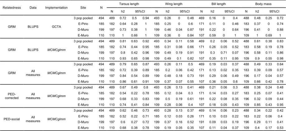
Heritability estimates
409
In general, heritability measures based on PED-social, PED-corrected and GRM, using
410
BLUPs or all the measurements, and with MCMCglmm or GCTA, were highly consistent
411
for the same trait (Table 2, Figure 3; see supplementary material 4 for variance
412
estimates associated with the other random factors). The variations were very high
413
among the three localities, for which sample sizes were very small. When pooling the
414
three localities, variations between methods and credible intervals decreased.
415
Considering estimates from MCMCglmm and models fitting all phenotypic
416
measurements, there was a consistent trend for lower heritability when using PED-social
417
compared to GRM (Figure 3). For example, tarsus length and body mass heritability
418
were lower by 22% and 31%, respectively, when using PED-social compared GRM.
419
Specifically, there was a trend for lower heritability when using social than
PED-420
corrected. For example, tarsus length and body mass heritability were lower by 7% and
421
11%, respectively, when using PED-social compared to PED-corrected. There was also
422
a trend for lower heritability when using PED-corrected compared to GRM. For example,
423
tarsus length and body mass heritability were lower by 15% and 22%, respectively,
424
when using PED-social compared to PED-corrected.
Heritability estimates were slightly higher when using BLUPs instead of all the
426
phenotypic measures, together with the GRM, in MCMCglmm (e.g. only 3% higher for
427
tarsus length, but 24% higher for body mass). Furthermore, credible intervals were
428
slightly higher when using BLUPs. Using BLUPs and the GRM in GCTA, heritability
429
estimates were relatively similar to the one obtained using MCMCglmm on all the
430
phenotypic measures and either the GRM or the PED-corrected.
431
The number of SNPs included to compute GRMs influenced the tarsus length
432
heritability estimates using either GCTA on BLUPs or MCMCglmm on all of the
433
phenotypic measures (Figure 4). For this trait, heritability sharply increased from a
434
handful of SNPs to approximately 5,000 SNPs. Heritability increased slowly from
435
approximately 5,000 to 15,000 SNPs and then reached a plateau along which a very
436
slow increase was however apparent. It is also worth mentioning a similarly shaped
437
increase of likelihood ratio tests from GCTA.
438 439
Genetic correlations between traits
440
In general, genetic correlations between traits calculated with the different methods,
441
were consistent for the same pair of trait (Table 3). However, the credible intervals were
442
generally large, with 13 of the 30 intervals including 0. The largest estimates and
443
smallest credible intervals were obtained for the genetic correlation between tarsus
444
length and body mass, the most heritable traits. For each pair of traits there was a trend
445
for a higher genetic correlation when using all measures than BLUPs.
446 447
Chromosome partitioning
When fitting the univariate GCTA model simultaneously on each autosome, the
449
correlation between heritability and chromosome length was positive for tarsus length (r2
450
= 0.26; p-value = 0.009), being the most heritable traits of this study. The correlation was
451
non-significant for body mass (r2 = 0.08; p-value = 0.20), wing length (r2 = 0.03; p-value
452
= 0.41), and bill length (r2 = 0.00; p-value = 0.85). Standard error intervals for
453
chromosome scaled heritability did not include zero only for chromosomes 1A and 3 for
454
tarsus length (Table 4, Figure 5), and for chromosome 6 for body mass. In the case of
455
tarsus length, no autosome had to be removed to enable the convergence of the model
456
fitting all the autosomes simultaneously. In contrast, for wing length, bill length and body
457
mass, the microchromosomes group had to be removed and respectively one, 12 and
458
three additional autosomes (by order of increasing size) had to be removed to enable
459
convergence of the models. When fitting the univariate GCTA model separately for each
460
autosome versus the rest of the genome, several heritabilities were likely overestimated
461
since the total heritability was larger than with the previous method (h2 = 1.47 vs 0.84
462
for tarsus length, 0.85 vs 0.36 for wing length, 1.11 vs 0.31 for bill length, and 0.95 vs
463
0.62 for body mass).
464 465
Discussion
466
Genomic analyses offer great opportunities for measuring relatedness precisely among
467
individuals from natural populations and hence estimating heritability and genetic
468
correlations among traits in the wild (Edwards 2013; Gienapp et al. 2017). Heritability
469
partitioning along the genome can also help in identifying regions explaining the additive
470
genetic variation for polygenic traits (Yang et al. 2011b). Determining trait heritability and
its partitioning along the genome, and understanding trait genetic covariances, are also
472
essential first steps to detect individual loci in the genome that contribute to trait
473
differences between individuals, using for example genome wide association or linkage
474
mapping (Schielzeth & Husby 2014). Although such approaches have been recently
475
tested in a few datasets of well-studied wild organisms (Robinson et al. 2013;
Stanton-476
Geddes et al. 2013; Bérénos et al. 2014), we require more explorations on whether
477
smaller datasets could be used for such procedures and on how they compare with the
478
classic animal model approach based on long-term pedigrees. In this context, we used
479
both social pedigrees (PED-social) and genome wide relatedness matrices (GRM), to
480
compute heritability estimates, genetic correlations, and chromosome partitioning for
481
several phenotypic quantitative traits (tarsus length, wing length, bill length, and body
482
mass) in a rather small dataset of individuals sampled in wild populations of Corsican
483
blue tits and genotyped at nearly 50,000 RADseq derived SNPs. We discuss the power
484
of such relatively small GRM, which may be typically produced while studying wild
485
populations of non-model species, to examine the aforementioned quantitative genetic
486
parameters.
487
Our main findings were i) a high congruence between heritability estimated using
488
GRM, PED-corrected and PED-social. However, the median heritability obtained using
489
the GRM was generally slightly higher than using PED-corrected and PED-social, which
490
may be attributed to absence of erroneous links, greater precision and higher
491
information content of the GRM. ii) The number of markers was not an issue for
492
computing the GRM and estimating heritability, when approximately 15,000 SNPs were
493
reached. iii) Genetic correlations among traits and chromosome partitioning were less
likely than heritability estimates to be very informative or robust given the large credible
495
intervals and the number of non-significant estimates, most likely due to power issues
496
(insufficient number of SNPs per chromosome in the case of the micro-chromosomes
497
and insufficient number of individuals). We thereafter discuss the usefulness and
498
limitations of inferences of quantitative genomic parameters, including heritability, in
499
relatively small sample sizes, with a medium number of genetic markers, for wild
500
populations of non-model species.
501 502
Comparing PED-social and GRM
503
The GRM obtained differed in two aspects from the PED-social (Fig 2D): higher density
504
and relatedness variance on one hand, and no pedigree errors on the other hand. The
505
first major difference was that the GRM enabled estimating relatedness among
506
individuals that were not connected in PED-social (Figure 2D; 460 GRM relatedness
507
values were higher than PED-social relatedness values by at least 0.1). This concerned
508
individuals at every degree of relatedness but obviously primarily among individuals from
509
disconnected families. Therefore, GRM increased the depth and also the size of the
510
pedigree. This illustrates the usefulness of GRM in cases for which a dense and deep
511
pedigree is difficult to obtain due to for example dispersal, large population size
512
compared to the fieldwork capacity, and family structure (Pemberton 2008).
513
Furthermore, GRM allows capturing much more variance in realized relatedness among
514
individuals, both close and more distantly related (Figure 2D), which may also increase
515
the power of such GRM-based estimates in large and open populations.
The second major difference between PED-social and GRM was that several
517
individuals had much higher relatedness in PED-social than in the GRM, most likely
518
indicating errors in PED-social. The most common cases consisted of wrongly assigned
519
parentages (relatedness of 0.5 in PED-social and 0 in GRM), half sibs most likely
520
originating from extra-pair paternities (relatedness of 0.5 in PED-social and 0.25 in
521
GRM), and the spread of such errors in the pedigree (other smaller relatedness in GRM
522
than in PED-social). Using this comparison between GRM and PED-social, we created a
523
PED-corrected in which these aforementioned erroneous links, accounting for
524
approximately 10% of the PED-social links, were corrected. This proportion of erroneous
525
linked corrected in our dataset should be expected since 18 to 25% of young have been
526
previously identified as extra-pair offspring in these Corsican blue tit populations
527
(Charmantier et al. 2004a).
528 529
Heritability estimates from PED-social, PED-corrected and GRM
530
Heritability estimated for tarsus length (0.62 to 0.81 depending on the method, for three
531
sites pooled, see Table 2) and body mass (0.34-0.61) were on the upper limit compared
532
to previous estimates in this species and for other close species (Jensen et al. 2008;
533
Husby et al. 2011; Postma 2014; Delahaie et al. 2017) while heritability for wing length
534
(0.26-0.34) and bill length (0.14-0.21) were rather on the lower ranges usually found.
535
Here again it should be noted that we did not optimize the animal models by integrating
536
factors that may have contributed to explain trait variation, for example to account for
537
daily and seasonal variation in body mass. Moreover, it has been observed that the
538
number of individuals included can affect the heritability estimates (Silva et al. 2017).
Credible intervals and standard errors for heritability estimates were much larger
540
than in previous studies based on larger sample size (Robinson et al. 2013;
Stanton-541
Geddes et al. 2013; Bérénos et al. 2014; Silva et al. 2017). The credible intervals per
542
site were larger than for the three sites pooled, suggesting the decrease of power with
543
decreasing sample size. Similarly, Silva et al. (2017) obtained increased standard errors
544
when decreasing sample size. This most likely suggests that the number of individuals
545
used here conferred limited power.
546
Overall, when using MCMCglmm and models using all of the phenotypic
547
measurements, heritability estimates were relatively similar for GRM, PED-corrected and
548
PED-social for the same trait (Figure 3). These results are in line with previous
549
comparisons realized with much larger sample size (Robinson et al. 2013; Bérénos et al.
550
2014). However, unlike these previous studies showing very small differences in
551
heritability based on PED-social and GRM, our estimates based on GRM were larger
552
than using PED-social and to a lesser extent, than using PED-corrected, for tarsus
553
length and for body mass, but not for wing length and bill length. Here, wing length
554
heritability was 0.28 using PED-social, 0.26 using PED-corrected and 0.26 using GRM
555
(Table 2). In turn, tarsus length heritability obtained from GRM was 18% higher than
556
from PED-corrected and the one from PED-corrected 8% higher than from PED-social.
557
Similarly, body mass heritability obtained from GRM was 29% higher than from
PED-558
corrected and the one from PED-corrected 12% higher than from PED-social. The
559
difference between PED-corrected and PED-social for these two traits may be
560
attributable to the erroneous links in PED-social. Indeed, it has been estimated that
561
PED-social containing 5 to 20% of extra-pair paternities result in underestimated
heritability by up to 17%, in blue tits (Charmantier & Réale 2005). Then, the differences
563
observed between heritability estimated using GRM and PED-corrected are likely to
564
originate from higher density of the GRM and the fact that GRM incorporate more
565
variance in relatedness for a given class of kinship. Further changing the pedigree by
566
not only correcting erroneous existing links but also informing previously unidentified
567
links (eg. linking previously unknown extra-pair fathers to their offspring) based on the
568
genetic data, could also decrease the heritability difference between PED-corrected and
569
GRM.
570
Heritability estimates, and their credible intervals, based on BLUPs were slightly
571
higher compared to estimates based on models using all phenotypic measurements
572
when using MCMCglmm (this was not true for GCTA). This is not surprising given that
573
BLUPs are known to artificially increase the precision of the measure and therefore
574
increase statistical significance (Hadfield et al. 2010). While the difference was low for
575
tarsus and bill length (3% and 5% higher, respectively), the difference was particularly
576
pronounced for wing length and body mass (31% and 24%, respectively). One
577
speculation is that wing length and body mass are less repeatable than tarsus length
578
and bill length and that our BLUPs did not adequately take into account individual
579
variance.
580 581
Effect of the number of SNPs on the heritability estimates based on GRM
582
The number of SNPs had a relatively minor effect on heritability estimates, from
583
approximately 15,000 SNPs (Figure 4). This is concordant with what has been shown in
584
previous studies (Stanton-Geddes et al. 2013; Bérénos et al. 2014). Of course, the effect
of the number of SNPs on the heritability estimation depends on several parameters
586
(e.g. genome size, LD across the genome, LD among markers, genetic architecture of
587
the focal trait, polymorphism of the markers, genotyping quality, missing data) and is not
588
transposable from one study to another. These days, the number of markers may no
589
longer be a problem, given the rise of the accessibility of many genomic tools. However,
590
the genotyping quality and missing data occurrence may be challenging for studies
591
using RADseq and GBS methods, as noted by (Gienapp et al. 2017). Here, we
592
prioritized the quantity and the quality of the RAD markers over the number of
593
individuals, as well as genotyping only individuals with high quality DNA, ending up with
594
a relatively high read depth and low missing rate. Future studies aiming to use RADseq
595
derived markers to estimate heritability should also find a tradeoff between the number
596
of genomic markers and the number of genotyped individuals. A formal simulation study
597
determining such a tradeoff between numbers of individuals and of markers and markers
598
read-depth (directly linked to quality) would be highly valuable for guiding the design of
599
RADseq analyses in the context of quantitative genomics.
600 601
Genetic correlations using PED-social, PED-corrected and GRM
602
Genetic correlations obtained using GRM, PED-social and PED-corrected had large
603
credible intervals, preventing us to make robust interpretations, except that our sample
604
size was probably too small to obtain acceptable credible intervals. This was partly
605
expected since bivariate models are known to be data hungry. While such lack of power
606
is a recurrent issue when estimating genetic correlations even with much larger sample
607
sizes (Vattikuti et al. 2012; Visscher et al. 2014; Ni et al. 2017), it was nevertheless a
disappointment while comparing these results to the one from (Bérénos et al. 2014), in
609
which the credible intervals were relatively small. The median values of genetic
610
correlations for these traits were in line with previous studies in other bird species
611
(Teplitsky et al. 2014).
612 613
Chromosome partitioning based on GRM
614
Chromosome partitioning of heritability of tarsus length was on par with what has been
615
observed in previous studies, i.e. increasing heritability of quantitative traits with
616
increasing number of genes per chromosome (Yang et al. 2011b; Robinson et al. 2013;
617
Santure et al. 2013, 2015; Bérénos et al. 2015; Wenzel et al. 2015; Silva et al. 2017).
618
Similarly to several of these previous studies, there were few chromosomes for which
619
standard error did not include zero. Of particular interest, chromosomes 3 and 1A
620
showed high heritability for tarsus length. These chromosomes may be of particular
621
interest for future studies investigating the genomic bases of this quantitative trait
622
variation in blue tits. Chromosome 3 was already identified in a recent study on
623
morphology of Dutch and British great tits (Santure et al. 2015) as explaining high
624
heritability for tarsus length. In contrast, chromosome 1A explained a low proportion of
625
genetic variance in this last study. These kind of discrepancies might be congruent with
626
the fact that this same study (Santure et al. 2015) also showed very little consistency
627
between the variance explained by each chromosome for great tit populations from the
628
Netherlands and from the United-Kingdom.
629
Regarding the three other traits analyzed, the chromosome partitioning results
630
appeared much less robust since several chromosomes had to be removed (7, 18, and
9 autosomes removed, for wing length, bill length and body mass, respectively) to
632
enable models’ convergence. The need for such chromosomes removals has previously
633
been reported (Wenzel et al. 2015; Silva et al. 2017) and has received detailed
634
consideration by Kemppainen & Husby (2018). In addition, the relationship between the
635
number of genes and the heritability explained by chromosomes were deviating from
636
theoretical expectations of increasing heritability with increasing chromosome size for
637
these polygenic traits. For comparison, Bosse et al. (2017) showed a significant increase
638
of the proportion of additive genetic variance of bill length explained by a chromosome in
639
relation to chromosome size in great tits. Such deviation may not have been affected by
640
removing chromosomes (Kemppainen & Husby 2018) but most likely originated from a
641
limited power of the small sample size, alongside relatively small heritabilities
642
(Kemppainen & Husby 2018).
643 644
Conclusion on the usefulness of GRM based heritability measures using small samples
645
from wild populations
646
Overall, our study reveals that RADseq data on around 50k SNPs (as advised by
647
Berenos et al 2014) for around 500 phenotyped individuals can provide estimates of
648
heritability that are close to, and probably more accurate than, estimates based on social
649
pedigree data from seven years monitoring for more than 1600 individuals (as included
650
in the PED-social used here). This opens very interesting avenues in the field of
651
quantitative genetics since estimating heritability and genetic correlations in the wild
652
have long been restricted to study systems where long-term monitoring is feasible.
653
RADseq data could allow the estimation of quantitative genetic parameters for a much
lower cost in terms of time (years) spent in the field, although individual capture and
655
phenotyping will most likely remain time consuming. Using GRM on few individuals gives
656
the power to estimate such parameters on virtually any species even though no
long-657
term pedigree is available (Gienapp 2017). This will notably allow moving on from
658
individual study to more comparative approaches and answer important questions such
659
as understanding the spatial variation of evolutionary potential or the role of evolutionary
660
constraints in phenotypic evolution. Such a genomic approach also provides the
661
possibility to explore genetic covariance between traits as well as chromosome
662
partitioning to confirm the polygenic architecture for phenotypic traits classically
663
measured in birds. Less than 500 individuals appears however to provide insufficient
664
power to correctly estimate either genetic covariances between traits or contribution of
665
individual chromosomes to overall heritability.
References
667
Andrews S (2010) FastQC: A quality control tool for high throughput sequence data.
668
Available online at: http://www.bioinformatics.babraham.ac.uk/projects/fastqc.
669
Baird NA, Etter PD, Atwood TS et al. (2008) Rapid SNP Discovery and Genetic Mapping
670
Using Sequenced RAD Markers. PLoS ONE 3(10): e3376.
671
https://doi.org/10.1371/journal.pone.0003376.
672
Bérénos C, Ellis PA, Pilkington JG, Pemberton JM (2014) Estimating quantitative
673
genetic parameters in wild populations: a comparison of pedigree and genomic
674
approaches. Molecular Ecology, 23, 3434–3451.
675
Bérénos C, Ellis PA, Pilkington JG et al. (2015) Heterogeneity of genetic architecture of
676
body size traits in a free-living population. Molecular Ecology, 24, 1810–1830.
677
Blondel J, Thomas DW, Charmantier A et al. (2006) A Thirty-Year Study of Phenotypic
678
and Genetic Variation of Blue Tits in Mediterranean Habitat Mosaics. Bioscience, 56,
679
661–673.
680
Bosse, M., Spurgin, L. G., Laine, V. N., Cole, E. F., Firth, J. A., Gienapp, P., ... &
681
Groenen, M. A. (2017). Recent natural selection causes adaptive evolution of an
682
avian polygenic trait. Science, 358, 365-368.
683
Catchen J, Hohenlohe PA, Bassham S, Amores A, Cresko WA (2013) Stacks: an
684
analysis tool set for population genomics. Molecular Ecology, 22, 3124–3140.
685
Charmantier A, Réale D (2005) How do misassigned paternities affect the estimation of
686
heritability in the wild? Molecular Ecology, 14, 2839–2850.
687
Charmantier A, Blondel J, Perret P, Lambrechts M (2004a) Do extra‐pair paternities
provide genetic benefits for female blue tits Parus caeruleus? Journal of Avian
689
Biology, 35, 1–9.
690
Charmantier A, Doutrelant C, Dubuc-Messier G, Fargevieille A, Szulkin M (2016)
691
Mediterranean blue tits as a case study of local adaptation. Evolutionary
692
Applications, 9, 135–152.
693
Charmantier A, Kruuk LEB, Blondel J, Lambrechts MM (2004b) Testing for
694
microevolution in body size in three blue tit populations. Journal of Evolutionary
695
Biology, 17, 732–743.
696
Csillery K (2006) Performance of Marker-Based Relatedness Estimators in Natural
697
Populations of Outbred Vertebrates. Genetics, 173, 2091–2101.
698
Danecek P, Auton A, Abecasis G et al. (2011) The variant call format and VCFtools.
699
Bioinformatics, 27, 2156–2158.
700
Delahaie, B., Charmantier, A., Chantepie, S., Garant, D., Porlier, M., & Teplitsky, C.
701
(2017). Conserved G-matrices of morphological and life-history traits among
702
continental and island blue tit populations. Heredity, 119, 76-87.
703
Edwards SV (2013) Next‐generation QTL mapping: crowdsourcing SNPs, without
704
pedigrees. Molecular Ecology, 22, 3885–3887.
705
Gagnaire, P. A., & Gaggiotti, O. E. (2016). Detecting polygenic selection in marine
706
populations by combining population genomics and quantitative genetics
707
approaches. Current Zoology, 62, 603-616.
708
Gienapp, P., Fior, S., Guillaume, F., Lasky, J. R., Sork, V. L., & Csilléry, K. (2017).
709
Genomic quantitative genetics to study evolution in the wild. Trends in ecology &
evolution, 32, 897–908.
711
Gosselin T (2017). Radiator: RADseq Data Exploration, Manipulation and Visualization
712
using R. doi: 10.5281/zenodo.154432.
713
Hadfield JD, Wilson AJ, Garant D, Sheldon BC, Kruuk LEB (2010) The Misuse of BLUP
714
in Ecology and Evolution. The American Naturalist, 175, 116–125.
715
Hadfield, J. D. (2010). MCMC methods for multi-response generalized linear mixed
716
models: the MCMCglmm R package. Journal of Statistical Software, 33, 1-22.
717
Huisman J (2017) Pedigree reconstruction from SNP data: parentage assignment,
718
sibship clustering and beyond. Molecular Ecology Resources, 17, 1009–1024.
719
Husby A, Hille SM, Visser ME (2011) Testing Mechanisms of Bergmann’s Rule:
720
Phenotypic Decline but No Genetic Change in Body Size in Three Passerine Bird
721
Populations. American Naturalist, 178, 202–213.
722
Jensen H, Steinsland I, Ringsby TH, Sæther B-E (2008) Evolutionary dynamics of a
723
sexual ornament in the house sparrow (Passer domesticus): the role of indirect
724
selection within and between sexes. Evolution, 62, 1275–1293.
725
Kemppainen, P., & Husby, A. (2018). Inference of genetic architecture from
726
chromosome partitioning analyses is sensitive to genome variation, sample size,
727
heritability and effect size distribution. Molecular Ecology Resources.
728
https://doi.org/10.1111/1755-0998.12774.
729
Kvist L, Viiri K, Dias PC, Rytkönen S, Orell M (2004) Glacial history and colonization of
730
Europe by the blue tit Parus caeruleus. Journal of Avian Biology, 35, 352–359.
731
Laine VN, Gossmann TI, Schachtschneider KM et al. (2016) Evolutionary signals of
732
selection on cognition from the great tit genome and methylome. Nature