A generalized variogram-based framework for multiscale ordination

HAL Id: hal-00016494

https://hal.archives-ouvertes.fr/hal-00016494

Submitted on 23 Feb 2006

HAL is a multi-disciplinary open access archive for the deposit and dissemination of sci-entific research documents, whether they are pub-lished or not. The documents may come from teaching and research institutions in France or abroad, or from public or private research centers.

L’archive ouverte pluridisciplinaire HAL, est destinée au dépôt et à la diffusion de documents scientifiques de niveau recherche, publiés ou non, émanant des établissements d’enseignement et de recherche français ou étrangers, des laboratoires publics ou privés.

Pierre Couteron, Sébastien Ollier

To cite this version:

Pierre Couteron, Sébastien Ollier. A generalized variogram-based framework for multiscale ordination. Ecology, Ecological Society of America, 2005, 86 (4), pp.828-834. �10.1890/03-3184�. �hal-00016494�

To be published in Ecology

Preprint version: January 6, 2005

A generalized, variogram-based framework for multi-scale

ordination

Pierre C

OUTERON1

and Sébastien O

LLIER2

1 Ecole Nationale du Génie Rural des Eaux et des Forêts / UMR botAnique et bioinforMatique de l’Architecture des Plantes (AMAP), Boulevard de la Lironde, TA40/PS2, 34398 Montpellier Cedex 05, France, and French Institute of

Pondicherry, 11 Saint Louis Street, Pondicherry 605001, India

2 UMR CNRS 5558, Laboratoire de Biométrie et Biologie Evolutive, Université Claude Bernard Lyon 1, 69 622 Villeurbanne Cedex, France.

Present address for direct correspondence

Pierre COUTERON

French Institute of Pondicherry, 11 Saint Louis Street, Pondicherry 605001, India Tel: +91 413 2334 168 , Fax: +91 413 2339 534

Abstract

Multi-scale ordination (MSO) deals with potential scale-dependence in species assemblages, by studying how results from multivariate ordination may be different on different spatial scales. MSO methods were initially based on two-term local covariances between species, and therefore required sampling designs composed of adjacent quadrats. A variogram-based MSO, applicable to very diverse sampling designs has recently been introduced by H.H. Wagner (2003, 2004). This refers to Principal Component Analysis, Correspondence Analysis and derived "two-table" (also called "direct") ordination methods, i.e., Redundancy Analysis and Canonical Correspondence Analysis.

In this paper we put forward an enlarged framework for variogram-based MSO which relies on a generalized definition of inter-species covariance and on matrix expression of spatial contiguity between sampling units. This enables us to provide distance-explicit decompositions of variances and covariances (in their generalized meaning), that are consistent with many ordination methods in both their single- and two-table versions. A spatially explicit apportioning of diversity indices is proposed for some particular definitions of variance. Referring to two-table ordination methods allowed the multi-scale study of residual spatial patterns after factoring out of available environmental variables. Some aspects of the approach are briefly illustrated with vegetation data from a neotropical rainforest in French Guiana.

Key words: diversity apportioning; species assemblages; multi-scale ordination; multivariate

geostatistics; canonical correspondence analysis; spatial contiguity; tropical rainforest; variogram.

Introduction

Determining to what extent multi-species patterns of association may be different on different spatial scales is obviously a central issue in ecology (Levin1992). The concern to integrate space in numerical studies of inter-species association has led to the development of a method of multi-scale ordination (MSO; Ver Hoef and Glenn-Lewin 1989). This requires data from continuous sampling designs (e.g. belt transects) since it is based on the computation of two- term local covariances between species (Greig-Smith 1983). In two recent papers, H.H. Wagner (2003, 2004) proposed a new method for MSO based on the variogram (Wackernagel 1998) thereby allowing the use of data collected by means of very diverse sampling designs. This insightful approach was proposed for two usual ordination methods, i.e., Principal Component Analysis (PCA) and Correspondence Analysis (CA). Extension to "direct" ordination methods (Legendre and Legendre 1998), using two data tables, such as Redundancy Analysis (RDA, relating to PCA) and Canonical Correspondence Analysis (CCA, relating to CA) was also proposed by Wagner (2004).

This most recent contribution is a considerable step forward since CA is generally preferred to PCA for the study of inter-species associations. CA is a very popular and powerful method that positions species and sites along common ordination axes, by applying the same centering and weighting options to rows and columns of the site by species table. However, in spite of several attractive properties, there is no reason to consider CA as being automatically the most appropriate ordination method whatever the characteristics of the data and the aim of the study (Gimaret-Carpentier et al. 1998). Several alternatives to CA, with distinct properties, can be defined by changing weighting options for either sites or species. For instance, Pélissier et al. (2003) demonstrated that changing species weighting, i.e. placing varying degrees of emphasis on scarce species, could be used to define three ordination methods (including CA) and that each was consistent with one classical diversity index (richness, Shannon's, Simpson's). On the other hand, Dolédec et al. (2000) used a uniform weighting of sites to derive an alternative to CCA with interesting properties for the separation of species niches. Hence, it would be preferable for ecologists to become aware of the potential adaptability of both single- and two-table methods of ordination to their specific aims and to the characteristics of their data. Such adaptability should also encompass the emerging field of spatially explicit ordinations.

The paper presented here was triggered by the pioneering work conducted by Wagner (2003, 2004) but aims to define a broader framework for variogram-based multi-scale ordinations. We intend to demonstrate that it is possible to partition by distance the results of very diverse ordination methods, as defined by re-scaling and weighting options for the rows and columns of the data tables. To do so, we will introduce a generalized definition of covariance between species which encompasses several ordination methods while being amenable to scale-explicit decompositions. Consistency with the additive decomposition of common diversity indices (Pélissier et al. 2003; Couteron and Pélissier 2004) will be highlighted, while referring to methods of two-table "direct" ordination will allows the explicit analysis of residual spatial patterns after the factoring out of some environmental variables. This aspect will be emphasized in a brief illustration based on vegetation data from a neotropical rainforest. In this report, we have chosen to keep mathematical developments to a minimum while providing a complete treatment in matrix form in an appendix published in the Electronic Ecological Archives. Computer programs are freely available from the first author (Matlab®

version) or on http://pbil.univ-lyon1.fr/CRAN/ (R [Ihaka and Gentleman 1996] version integrated in the ade4 package).

A generalized definition of covariance

Data tables containing counts of individual organisms by sampling sites (say "quadrats") and taxa (usually species) are both a central and general feature of ecological studies. Let us consider such a table, based on N sampled individuals, for which fai is the total number of

individuals belonging to species i (1<i<S) that were counted in quadrat a (1<a<Q). Let pai be

the corresponding relative frequency (pai=fai/N) while pa+ and p+i are the relative frequencies

for quadrat a and species i, respectively. We have introduced our topic with explicit reference to counted individuals, though the above parameters remain meaningful as long as fai is a

non-negative value (biomass measurements, semi-quantitative indices of abundance, presence/absence, …) expressing the abundance of species i in quadrat a.

Ordination methods such as correspondence analysis CA and various versions of PCA (ter Braak 1983) are the usual tools employed to analyze quadrats by species tables. Central to all these methods is the application of singular values decomposition (svd), also called eigenanalysis, to a square S by S matrix, which is the usual variance-covariance matrix, C, for the species-centered (non-standardized) PCA and which is another matrix Q² in the case of CA (see Legendre and Legendre 1998:453 and Wagner 2004 for details). In Q², terms on the diagonal are homologous to variances and are proportional to the portions of the total chi-square of the data table (Legendre and Legendre 1998:452) that are attached to each of the S species. Off-diagonal terms are homologous to the usual pairwise covariances and measure to what extent two arbitrary species may conjointly depart from expected abundance values. We can see matrices C and Q² as nothing more that special cases of a square matrix

based on an appropriate generalization of the notions of species variance (diagonal values) and covariance (off-diagonal values). This generalized measure of covariance is, for two arbitrary species i and j:

[ ]

gij S j 1 S, i 1 ≤≤ ≤≤ = T G

∑∑

= = − − = Q a Q b b a bj aj j i bi ai ij x x ww x x g 1 1 ) ( ) ( 2 1 _{δ δ} (1)

variance being a special case with i=j.

Here, wi weighs the influence of species i, while δa and δb are the weights given to quadrats a

and b, respectively; xai denotes any measure of abundance of species i in quadrat a that can

be derived from the initial value fai via re-scaling options (Table 1).

The choice of weighting options is a central yet often eluded question when using multivariate techniques, since weighting along with re-scaling and centering defines the nature of the distance between quadrats and, for some methods, also between species. Moreover, the choice of weighting options relates to very practical questions concerning, for instance, the influence that it seems meaningful to confer to a particular species in the definition of a multi-specific assemblage, or to a given quadrat in the investigation of an ecological gradient. Addressing such questions means that the biogeographic context must be taken into account (e.g., are there many scarce species? How abundant are the most frequent species?) along with the sampling design (does it give a fair estimate of species abundance in a region?) and, for two-table methods, the nature of the ecological gradients under study (are there strong limiting factors or threshold effects?). More detailed discussions on the consequences of weighting can

be found in Dolédec et al. (2000, regarding quadrats in direct gradient analysis) and in Pélissier et al. (2003, regarding species).

Combining re-scaling and weighting options opens up a wide selection of ordination methods and associated properties. Some examples, based on published methods, are presented in Table 1, but other possibilities are obviously imaginable. The presentation of classical ordination methods in terms of weighting of rows and columns was introduced by Escoufier (1987) and was used by Sabatier et al. (1989) and Dolédec et al. (2000) for several single- and two-table methods (including CA, CCA and classical versions of PCA and RDA). Pélissier et al. (2003) used this presentation to compare the properties of the three methods corresponding to option IV in Table 1, and to investigate their relationship with diversity measures. All these authors based their presentation of the methods on a species-centered version of the data table containing differences between individual observations, xai, and the δa-weighted mean

value,x , found for each species. Alternatively, in Eq. 1, we use all pairwise differences i between observations to compute variance and covariance. The equivalence of the two approaches is explained in the appendix (see Eq. A.5 to Eq. A.10).

Generalized spatial covariance

From Eq. 1, the contribution made by a given pair (a,b) of quadrats to the covariance between

two species can be expressed as: b a bj aj j i bi ai ij a b x x ww x x g ( ) ( )δδ 2 1 ) , ( = − − (2)

This translates easily into a generalized version of cross-variograms (i≠j) and variograms

(i=j), namely:

∑

≈ = h h b a ij ij ab b a g h K h , ) , ( ) ( 1 ) ( G γ (3)

where h is the central value of a given distance class, and where K(h) is a scaling coefficient, such as:

∑

≈ = h h b a b a ab h K , ) ( δ δ (4)

Considering all species together leads to a generalized variogram of species composition ("generalized" since potentially relating to several ordination methods and distance metrics):

∑

= i ii h h) ( ) ( G G

γ

γ

(5)

Eq. 4 is a crucial point since K(h) standardizes

γ

G(h)in such a manner to equate its expected

value (sill) with the total variance of the ordination method defined by weighting options. This is completely different from computing the usual experimental variogram from ordination scores, except for the special case of uniform quadrat weights (as in Wagner 2003) where K(h) is proportional to the number, nh, of pairs of quadrats relating to distance class h.

Conversely, if quadrat weights are not uniform, scaling by K(h) is the only manner to ensure that, whatever the distance class, the expected value of

γ

G(h) is the total variance ("inertia")

attached to matrix GT and computed from the sum of its diagonal elements. Note that such a

property is not guaranteed by the manner in which Wagner (2004) defined her version (denoted as

γ

Q(h)) of the CA-related variogram since the corresponding scaling remains

proportional to nh despite the fact that quadrat weights are not uniform. The scaling by K(h) is

diversity measurement (option IV in Table 1). In this case, the trace of GT is the diversity

among quadrats (Couteron and Pélissier 2004), which means that

γ

G(h) measures the average

beta-diversity between pairs of quadrats corresponding to distance class h. Equivalently,

∑

= i ii a b g b a VAR( , ) ( , ) (6)

quantifies the contribution made by a given couple (a,b) of quadrats to beta-diversity. Some classical dissimilarity indices, such as Jaccard's or Sorensen's (Legendre and Legendre 1998:256) are often used to quantify beta-diversity, though these have no direct connection with either geostatiscal tools or ordination methods. Conversely, Eqs.2 and 6 provide a family of dissimilarity indices some of which relate directly to both.

Variograms and cross-variograms of ordination axes

Regardless of the reference ordination method chosen, a generalized variance-covariance matrix, Gh, is computed for each distance class h. To ensure efficient computations by any matrix-oriented programming language, as we did with Matlab® and R (Ihaka and Gentleman 1996), we introduced a matrix formulation of the method. It is based of a contiguity relationship (Thioulouse et al. 1995) consistent with the variogram, which considers two quadrats as "neighbors at scale h" if the distance between them is within the bounds of the class centered around h (see Appendix). Assuming that distance classes include all pairs of quadrats while being mutually exclusive, we demonstrated (see Appendix, Eq. A.13) that the matrices Gh sum to GT, whatever the initial choice of the reference ordination method by

weighting options.

The eigenvectors and eigenvalues originating from the singular values decomposition (svd) of

GT can be partitioned with respect to distance classes (Appendix), as a generalization of the

fundamental principle introduced by Ver Hoef and Glenn-Lewin (1989). But the complete variance-covariance matrix, Fh, between eigenvectors can also be obtained (Appendix, Eq. A.13). Considering off-diagonal elements of Fh, namely covariances at scale h between eigenvectors, is a new perspective in MSO which can be used to investigate the potential existence of a scale-dependent covariance between distinct ordination axes. This question, though ignored by most papers devoted to MSO, is closely related to the initial concern of Noy-Meir and Anderson (1971), namely that ordination results may substantially vary with spatial scales. This would mean, for example, that species displaying the most prominent variations of abundance may not be the same depending on the average distance between the quadrats, or that distinct species assemblages may be found for different distance classes. How can we test whether this is the case or not? One way would be to carry out an ordination for each of the Gh matrices and compare the results, but this is likely to be cumbersome while objective criteria for the comparison are not straightforward to define. We propose a more efficient approach by constructing cross-variograms of eigenvectors from the off-diagonal values of Fh matrices after appropriate scaling by K(h). All these cross-variograms have an expectation of zero, since the eigenvectors of GT are globally uncorrelated, but some may

have significant departures from this expectation on particular scales. (Of course, only the cross-variograms for the most prominent eigenvectors are to be analyzed.) If this is the case, it is possible to know at which scales it may be worthwhile carrying out specific ordination analyses via the svd of the corresponding Gh matrices.

Taking environmental heterogeneity into account

If the species by quadrats table is accompanied by environmental variables assessed at the quadrat scale, it is advantageous to factor out the influence of such variables prior to analyzing the residual spatial patterns of species composition. Technically, this verifies whether some basic assumptions, such as "intrinsic" stationarity (used to interpret the empirical variogram), or independence of residuals (assumed to fit a linear model of species-environment relationship) are met by the data (see Wagner 2004 for an extensive discussion). In terms of ecological interpretation, it is judicious to see residual spatial patterns of community composition as predominantly shaped by biotic processes, such as species dissemination or species interactions (Wagner 2004) and as potentially informative on the scale at which such processes may operate.

Any two-table "direct" ordination starts from the decomposition of the quadrats by species table, X, into an approximated table A, modelled from environmental variables by a weighted

linear regression and a residual table R. Such a decomposition may be carried out in a manner

consistent with a two-table version of any of the ordination methods mentioned in Table 1 (Sabatier et al. 1989; Pélissier et al. 2003) when the linear regression uses the quadrat weights defining the ordination. (For instance, defining table X along with species and quadrat

weights so as to make them consistent with CA means that an ordination on A would be a

CCA.) To study residual spatial patterns, it is possible to break down GR, i.e., the

variance-covariance matrix computed from R, into additive variance-covariance matrices, GRh, each

corresponding to a certain distance class, and on which a variogram-based multi-scale analysis can be based (see Appendix).

Brief illustration based on tropical rain forest data

We considered 7,189 trees (diameter at breast height above 10 cm) belonging to 59 species sampled in a lowland tropical rain forest of ca. 10, 000 ha in French Guiana. The sampling design was based on 411 rectangular quadrats of 0.3 ha each, located at the nodes of a 400 m by 500 m grid. Environmental information at the quadrat scale was expressed by a synthetic nominal variable (12 categories) primarily based on topography and soil water regime (see Couteron et al. 2003 for details). Performing CA on the quadrats by species table showed two main floristic gradients corresponding to the second and third axes (CA2 and CA3). The first axis (CA1) resulted from the spurious occurrence of a scarce species (17 trees) in a particular quadrat and this illustrates a well-known drawback of CA. Results of the non-symmetric correspondence analysis (NSCA) were free from this problem, while the two main axes, NSCA1 and NSCA2, correlated strongly with CA3 and CA2 (r = 0.76 and r = 0.84, respectively) despite being defined from distinct species. For this data set, shifting emphasis from scarce to abundant species changed the hierarchy between the ordination axes, but the detection of two main floristic gradients proved robust with respect to species weighting. To go beyond these results established by a previous study (Couteron et al. 2003) we explicitly considered inter-quadrats distances by applying the generalized variogram-based MSO with CA and NSCA as reference ordination methods. First, we partitioned the total variance attached to each ordination axis (eigenvalue) among distance classes. Since diversity-related ordinations were used (Pélissier et al. 2003), it was the total among-quadrats diversity (sensu the species richness for CA or the Simpson-Gini index for NSCA) which was successively broken down with respect to main floristic gradients (eigenvalues) and distance classes.

The floristic gradient defined by CA2 and NSCA2 failed to show any obvious spatial pattern since variograms were found to waver between confidence envelopes, and this regardless of the reference ordination (Fig. 1-a and b). The study of residual patterns, after factoring out the 12 environmental categories (unconstrained ordinations on the residual variance-covariance matrix, R) showed significant departures of the CA-based variogram for distances under 2

km. Such a change in the variogram stemming from the partialling out of the environmental variable typifies the complex interaction which can be expected between the environmental heterogeneity and spatial patterns of species assemblages. It also illustrates the advantage of studying such an interaction within a unified theoretical framework of multi-scale ordination since it enabled us to express in the same unit all kinds of results derived from a particular ordination method. This renders variograms of both initial and residual patterns directly comparable, i.e. a desirable property that could not have been achieved by the computation of classical variograms from ordination scores. The other floristic gradient (defined by CA3 and NSCA1) showed a strong spatial pattern that pointed toward non-stationarity (see Wagner 2004 for a detailed definition) since both initial variograms (Fig. 1-c and 1-d) continued to rise up to 8 km without reaching a sill. The variograms of the homologous axes provided by CA and NSCA after factoring out the qualitative environmental categories appeared to be very similar. This indicated that the observed spatial patterns relating to this floristic gradient were not determined by the spatial distribution of the environmental categories.

By separately analyzing spatial patterns of distinct ordination axes we have implicitly hypothesized the absence of any scale-dependent relationship between the ordination axes or, equivalently, the stability across scales of inter-species covariances (“intrinsic” covariances

sensu Wackernagel, 1998). Such a hypothesis can be easily addressed by computing the

cross-variograms between the ordination axes (from off-diagonal elements of matrices Fh,Eq. A.18

in the Appendix). Only cross-variograms computed from the residual variance-covariance matrix (R) are shown (Fig. 1-e and –f) since homologous cross-variograms from the initial

data table were very similar. No scale dependence was observed between the two ordination axes given by NSCA (Fig. 1-f) and covariances between abundant species thus appeared to be stable across scales. This was not the case when the emphasis was placed on scarcer species by the use of CA since most values of the corresponding cross-variogram were outside the confidence envelopes (Fig. 1-e). Indeed, by diagonalizing the pooled variance-covariance matrices for distances under 4 km vs. distances above 4 km, we obtained two clearly distinct sets of species with high loadings on the ordination axes (results not shown). This result exemplified how scale-dependence may be detected by analyzing cross-variograms between ordination axes, while also illustrating the influence that species weighting may have: CA results proved scale-dependent though NSCA results did not.

Concluding remarks

In the above illustration, we deliberately restricted ourselves to some particular analyses that can be obtained from the generalized variogram-based MSO, but other kinds of analyses are clearly possible. For instance, it may be of interest to compare the spatial patterns of all individual species and identify scales on which some patterns may differ from others. This can be done by analysing, for instance by PCA, the table containing the generalized variograms of all species (prior standardization by variances of individual species as to have all sills equal to one is likely to be preferable). It may also be of interest to study the manner in which the distribution of the eigenvalues changes with scale, by analyzing the table

containing the generalized variogram of the eigenvalues. Any type of MSO can address these questions, but our unifying approach also provides a choice between ordination methods while offering links with diversity measurement and apportioning. As a consequence, future users may be able to select the particular ordination method (either direct or indirect) that best suits their data and aims.

Furthermore, the presentation of the method in matrix-form, with the use of contiguity matrices (Appendix), not only allows forefficient programming, but also opens up interesting methodological perspectives. Indeed, two-term local variances and covariances (TTLV/TTLC) on which the "classical" MSO relies (Ver Hoef and Glenn-Lewin 1989) have been also formulated using contiguity matrices (Di Bella and Jona-Lasinio 1996, Ollier et al. 2003). Such a formulation is obviously a sound basis, not only for a further generalization of the TTLV/TTLC-based MSO, as performed by us with the variogram-based MSO, but also for a thorough investigation of the respective properties of the two approaches.

Acknowledgements

We are indebted to D. Chessel (University of Lyon-1) for important insights into several topics mentioned in this paper, to R. Pélissier (IRD/UMR AMAP) for his valuable comments on preliminary drafts, and to H. H. Wagner for pertinent comments on the initial version.

Literature cited

Couteron, P., and R. Pélissier. 2004. Additive apportioning of species diversity: towards more sophisticated models and analyses. Oikos, 107: 215-221..

Couteron, P., R. Pélissier , D. Mapaga, J.-F. Molino, and L. Teillier. 2003. Drawing ecological insights from a management-oriented forest inventory in French Guiana. Forest Ecology and Management 172:89-108.

Di Bella, G., and G. Jona-Lasinio. 1996. Including spatial contiguity information in the analysis of multispecific patterns. Environmental and Ecological Statistics 3: 269-280.

Dolédec, S., D. Chessel, and C. Gimaret-Carpentier. 2000. Niche separation in community analysis: a new method. Ecology 81:2914–2927.

Escoufier, Y. 1987. The duality diagram: a means of better practical applications. Pages 139-156 in P. Legendre and L. Legendre, editors. Development in numerical ecology. Springer-Verlag, Berlin, Germany.

Gimaret-Carpentier, C., D. Chessel, and J.-P. Pascal. 1998. Non-symmetric correspondence analysis: an alternative for species occurrences data. Plant Ecology 138:97–112.

Greig-Smith, P. 1983. Quantitative Plant Ecology. 3rd _{ed. Blackwell Science Publishing,}

Oxford, UK.

Ihaka, R., and R. Gentleman. 1996. R: a language for data analysis and graphics. Journal of Computational and Graphical Statistics 5:299-314.

Legendre, P., and L. Legendre. 1998. Numerical ecology. Elsevier, Amsterdam, The Netherlands.

Noy-Meir, I., and D. Anderson. 1971. Multiple pattern analysis or multiscale ordination: towards a vegetation hologram. Pages 207-232 in G. P. Patil, E.C. Pielou, and E.W. Water, editors. Statistical ecology: populations, ecosystems, and systems analysis. Pennsylvania State University Press, University Park, Pennsylvania, USA.

Ollier, S., D. Chessel, P. Couteron, R. Pélissier, and J. Thioulouse. 2003. Comparing and classifying one-dimensional spatial patterns: an application to laser altimeter profiles. Remote Sensing of Environment 85: 453:462.

Pélissier, R., P. Couteron, S. Dray, and D. Sabatier. 2003. Consistency between ordination techniques and diversity measurements: two strategies for species occurrence data. Ecology, 84:242-251.

Sabatier, R., J.-D. Lebreton, and D. Chessel. 1989. Principal component analysis with instrumental variables as a tool for modelling composition data. Pages 341–352 in R. Coppi and S. Bolasco, editors. Multiway data analysis, Elsevier Science Publishers, The Netherlands.

ter Braak, C. J. F. 1983. Principal components biplots and alpha and beta diversity. Ecology 64: 454-462.

Thioulouse, J., D. Chessel, and S. Champély. 1995. Multivariate analysis of spatial patterns: a unified approach to local and global structures. Environmental and Ecological Statistics

2: 1-14.

Ver Hoef, J. M., and D. C. Glenn-Lewin. 1989. Multiscale ordination: a method for detecting pattern at several scales. Vegetatio 82: 59-67.

Wackernagel, H. 1998. Multivariate geostatistics. Second completely revised edition. Springer, Berlin, Germany.

Wagner, H. H. 2003. Spatial covariance in plant communities: integrating ordination, geostatistics, and variance testing. Ecology 84: 1045-1057.

Wagner, H. H. 2004. Direct multi-scale ordination with canonical correspondence analysis. Ecology 85: 342-351.

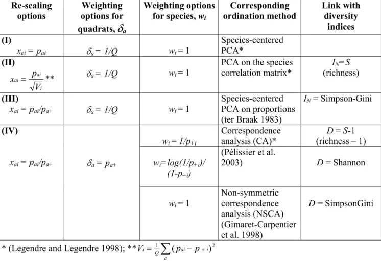
Table 1. Definition of some ordination methods from re-scaling and weighting options

D is the total diversity computed from the species frequency distribution

( =

∑

+ − ₊ , while I

i i

i

i f f

w

D [ (1 )] N is the total "inertia" corresponding to the ordination of the

species by quadrats table (trace of the generalized variance-covariance matrix, GT). See text

for other denotation.

Re-scaling options Weighting options for quadrats,

δ

a Weighting options for species, wi Corresponding ordination method Link with diversity indices (I) xai = pai δa = 1/Q wi = 1 Species-centered PCA* (II) i ai ai V p x = ** δa = 1/Q wi = 1

PCA on the species correlation matrix* IN=S (richness) (III) xai = pai/pa+ δa = 1/Q wi = 1 Species-centered PCA on proportions (ter Braak 1983) IN = Simpson-Gini wi = 1/p+i Correspondence analysis (CA)* D = S-1 (richness – 1) wi=log(1/p+i)/ (1-p+i) (Pélissier et al. 2003) D = Shannon (IV) xai = pai/pa+ δa = pa+ wi = 1 Non-symmetric correspondence analysis (NSCA) (Gimaret-Carpentier et al. 1998) D = SimpsonGini

* (Legendre and Legendre 1998); ** =

∑

− + a i ai Q i 1 (p p )2 V

Legend for Figure 1

Spatial patterns shown by the main ordination axes provided by the application of correspondence analysis (CA) and non-symmetric correspondence analysis (NSCA) to

vegetation data from the Counami Forest Reserve in French Guiana (7,189 trees of 59 species sampled in 411 quadrats of 0.3 ha each). a) Generalized variogram for axis CA2 of the initial table (filled circles) and for the homologous axis from the residual table, after factoring out of 12 environmental categories (open circles). The dashed lines denote the 95% bilateral

envelopes computed from 300 re-allocations of the specific composition to geographical locations (complete randomization for variograms from the initial data table and

randomization within environmental categories for variograms from the residual table). The dotted line denotes the mean values for randomizations. b) Same as a) but for axis NSCA2. c) Same as a) but for CA3 (confidence envelopes are omitted for legibility, values within envelopes are marked by a square). d) Same as a) but for NSCA1. e) Generalized cross-variograms between the two main CA axes of the residual table. f) same as e) for NSCA.

2 4 6 8 0 .1 5 0 .2 5 0 .3 5 0 .4 5 2 4 6 8 0 .0 0 4 0 .0 0 6 0 .0 0 8 0 .0 1 0 0 .0 1 2 2 4 6 8 0 .1 0 0 .2 0 0 .3 0 0 .4 0 2 4 6 8 0 .0 2 0 .0 3 0 .0 4 0 .0 5 0 .0 6 0 .0 7 2 4 6 8 -0 .0 6 -0 .0 2 0 .0 2 0 .0 6 2 4 6 8 -0 .0 0 2 0 .0 0 0 0 .0 0 1 0 .0 0 2

Figure 1

d)

b)

f)

a)

γ

G

ii

(h

)

c)

γ

Gii

(h)

Distance h (km)

e)

γ

Gij

(h)

Distance h (km)

CA

NSCA

Ecological Archives E086-042-A1

Pierre Couteron, and Sébastien Ollier. 2005. A generalized, variogram-based framework for multi-scale ordination. Ecology 86:828-834.

Appendix A. Matrix-algebraic presentation of the concepts and computations..

General denotation

Let X be a table expressing a measure of the abundance xai of S species (columns) within Q

quadrats (rows). xi and xj are two columns of table X, relating to species i and j, respectively.

Let D be a matrix containing quadrat weights (δa ,

∑

=1

a a

δ ) on its main diagonal and zeros for all off-diagonal values, and let W be a S by S matrix containing the square root of species weights ( w ) on its main diagonal and zeros outside. (In the main paper, Table 1 gives i some options for abundance re-scaling and for quadrat and species weighting.)

Contiguity relationships

Let Lh be a Q by Q matrix expressing a contiguity relationship (sensu Lebart 1969) between

the quadrats. For our variogram-based approach, we consider quadrats a and b as neighbors if the distance between the two is within the bounds of the distance class centered around h:

Lh(a,b)=1 if ha,b≈h and Lh(a,b)=0 otherwise. (A.1)

To introduce quadrat weights into the analysis, we define the matrix Mh and the vector Eh

such that:

D DL

Mh= h and Eh=Mh1Q (A.2)

where 1Q is the vector containing Q values equal to 1.

Mh contains, for each pair (a,b) of neighboring quadrats at "scale" h, the product δaδb of their

weights. Eh features, for each quadrat a, the sum of the weights of its neighbors multiplied by

∑

= h h M MT and =

∑

(A.2b) h h N NT

are such that MT is a Q by Q matrix that containing zeros on the diagonal while all values off

the diagonal are equal to δaδb; NT is a Q by Q matrix that containing (1-δa)δa values on the

diagonal and zeros elsewhere. With MT and NT it is as if each quadrat has all other quadrats as

neighbors. Denoting IQ the Q by Q diagonal identity matrix, we can also write: D)

D(I

NT= Q− and MT=D(1Q1Qt−IQ)D (A.3) (where the exponent ' t ' is the matrix transpose). Thus:

D 1 D1 D M N t T T− = − Q Q (A.4)

Equivalent expressions of the generalized variance-covariance matrix

Let GT be the generalized variance-covariance matrix, irrespective of distance classes, that

can be directly computed from table X using weighting options for rows and columns defined

by matrices D and W, respectively. GT contains, for each species couple (i,j), the generalized

covariances, gij as defined by Eq. 1 and Eq. 2 in the main paper:

∑

= b a ij ij g a b g , ) , ( (A.5)

Usual algebraic manipulations allow us to re-write Eq. 1 and Eq. A.5 as:

⎟⎟ ⎠ ⎞ ⎜⎜ ⎝ ⎛ =

∑

ai aj− i j Q a a j i ij ww x x xx g δ (A.6)

where x and i xjare the D-weighted means of xi and xj, respectively.

( ia Q a a i x x =∑δ or, equivalently, xi=XitD1Q) The matrix expression of gij is thus:

W D1 x D1 x Dx W(xit j it Q jt Q) ij g = − (A.7)

which generalizes into:

W X D X DX W(X GT= t − t ) (A.8) where X 1 1 tDX Q Q

= and where XtDX=

[ ]

xixj (A.9) Note that we may also write:

W X X D X X W GT= ( − )t ( − ) (A.10)

)XW M (N WX

GT= T− T (A.11)

Proof of Eq. A.11:

D)X 1 D1 (D X )X M (N

Xt T− T = t − Q Qt (using Eq. A.4)

X D X DX X D)X 1 D1 (D X t t t Q Q

t _{− = − (using Eq. A.9)}

Noting that XtDX₌XtDX_{, allows us to write:} X D X DX X )X M (N Xt T− T = t − t (A12)

Partition of the generalized variance-covariance matrix among distance classes

The very definition of matrices NT and MT (Eq. A.2b), along with Eq. A.11, enables partition

of GT into strictly additive components, Gh, that relate each to a distance class:

∑

=

∑

− = h h h h h WX N M XW G G t T ( ) (A.13)

Gh is the generalized variance-covariance matrix defined for the distance class h by the

neighboring relationship expressed by the matrices Nh and Mh. Gh translates easily into

generalization of Wagner's variogram matrix (2003) by a division of all its values by

∑

≈ = h h b a b a ab h K , ) ( δ δ or K(h)=1QtMh1Q (A.14) Equations A.2, A.13 and A.14 are used for easy programming of the method as well as efficient computations via any matrix-oriented programming environment, as we did with Matlab® and R (Ihaka and Gentleman 1996): see the freely available library "msov" on

http://pbil.univ-lyon1.fr/CRAN/.)

For a particular species couple i and j we obtain:

W x M N Wxt j h h i ij h g ( )= ( − ) (A.15)

Dividing by the scaling factor K(h) gives the value at "scale" h of the generalized version of either cross-variogram (i≠j) or variogram (i=j) :

) ( ) ( 1 ) ( g h h K h ij ij = G

γ

(A.16)

All the ordination methods mentioned in Table 1 of the main paper are based on the singular values decomposition (svd) of the appropriate version of GT to compute eigenvectors, uf, and

associated eigenvalues, λf. Let Uf be the matrix having all the eigenvectors uf as columns and

let Λ be the diagonal matrix having the eigenvalues λf on its diagonal. Both eigenvectors and

eigenvalues of GT can be partitioned by distance classes:

f h t f h U GU F = and λf(h)=uftGhuf (A.17)

Fh is the variance-covariance matrix of the eigenvectors at scale h. Scale-dependent

variogram/cross-variogram matrices of the eigenvectors are deduced by the appropriate scaling (Eq. A.16). Note also that:

Λ U G U U G U F ⎟ = T = ⎠ ⎞ ⎜ ⎝ ⎛ =

∑

∑

f ft f h h t f h h (A.18)

Taking environmental heterogeneity into account

Let us now suppose that a table, Z, containing assessments of P environmental variables for

the Q quadrats, is available in addition to table of species composition. It is well established that the centered by columns table,XC, may be partitioned into an approximated table,

C C Z(Z DZ) Z DX

A ₌ t −1 t _(A.19)

and a residual table, RC=XC−Ac (Sabatier et al. 1989).

In the same manner, it may also have a direct decomposition of the initial table X: )X M (N Z )Z) M (N Z(Z A= t T− T −1 t T− T and R=X−A (A.20)

After factoring out the environmental variables, residual spatial patterns may be studied by the multi-scale analysis of spatial covariances derived from table R or . The total residual variance-covariance matrix, G C R RT, is computed as: W )R M (N WR )RW M (N WR GRT= t T− T = Ct T− T C (A.21)

and is broken down with respect to distance classes:

W )R M (N WR )RW M (N WR GRh= t h− h = Ct h− h C (A.22)

The additive partitioning of GRT with respect to distance classes thus enables an investigation

of the residual spatial patterns by a multi-scale ordination scheme analogous to that defined by Eq. A.17 and Eq. A.18.

Ihaka, R., and R. Gentleman. 1996. R: a language for data analysis and graphics. Journal of Computational and Graphical Statistics 5:299-314.

Lebart, L. 1969. Analyse statistique de la contiguïté. Publications de l'Institut de Statistiques de l'Université de Paris 28: 81-112.

Sabatier, R., J.-D. Lebreton, and D. Chessel. 1989. Principal component analysis with instrumental variables as a tool for modelling composition data. Pages 341–352 in R. Coppi and S. Bolasco, Editors. Multiway data analysis, Elsevier Science Publishers, Amsterdam, The Netherlands.

Wagner, H.H. 2003. Spatial covariance in plant communities: integrating ordination, geostatistics, and variance testing. Ecology 84: 1045-1057.