Demonstration of Bayesian inference and Bayesian experimental design in a model film/substrate inference problem

Demonstration of Bayesian inference and Bayesian

experimental design in a model film/substrate

inference problem

by

Raghav Aggarwal

Submitted to the Department of Mechanical Engineering

in partial fulfillment of the requirements for the degree of

Master of Science in Mechanical Engineering

at the

MASSACHUSETTS INSTITUTE OF TECHNOLOGY

June 2016

@

Massachusetts Institute of Technology 2016. All rights reserved.

Author...

Certified by...

Signature redacted

_...

Department of Mechanical Engineering

May 20, 2016

Signature redacted

Michael J. Demkowicz

Certified by..

Certified by

Signature redacted

(

Signature redacted

Associate Professor

Thesis Supervisor

Youssef M. Marzouk

Associate Professor

Thesis Supervisor

Accepted by ...

MASSACH E NSTITUTE OF TECHNOLOGY

JUN 0

2

2016

~fl

(

--

Nicolas Hadjiconstantinou

Professor

C-1 A

Thesis Reader

Signature redacted

...

ORohan Abeyaratne

Chair, Committee on Graduate Students

Demonstration of Bayesian inference and Bayesian

experimental design in a model film/substrate inference

problem

by

Raghav Aggarwal

Submitted to the Department of Mechanical Engineering on May 20, 2016, in partial fulfillment of the

requirements for the degree of

Master of Science in Mechanical Engineering

Abstract

In this thesis, we implement Bayesian inference and Bayesian experiment design in a model materials science problem. We demonstrate that by observing the behavior of a film deposited on a substrate, certain features of the substrate may be inferred, with quantified uncertainty. We show that Bayesian experimental design can be used to design efficient experiments. The substrate in this model problem is a Gaussian random field, and the film is a phase separating mixture modeled by the Cahn-Hilliard equation. A key feature of the inference and the experiment design is a stochastic reduced-order model.

Thesis Supervisor: Michael J. Demkowicz Title: Associate Professor

Thesis Supervisor: Youssef M. Marzouk Title: Associate Professor

Acknowledgments

This work was funded by the US Department of Energy, Office of Basic Energy Sciences under award no. DE-SC0008929

Contents

1 Introduction 11

2 Model system 15

2.1 Substrate ... ... 15

2.1.1 Generating the substrate . . . . 16

2.2 F ilm . . . . 19

2.2.1 Solving the Cahn-Hilliard equation . . . . 20

2.3 Film-substrate interaction . . . . 23

2.4 Reduced order model . . . . 26

3 Bayesian inference 31 3.1 Inferring f . . . . . .32 3.2 Inferring 6 . . . . 35

4 Bayesian experimental design 39 4.1 Objective functions . . . . 39

4.2 Numerical approximation . . . . 40

4.3 Experimental design for inference of f . . . 42

List of Figures

2-1 (a) Uniform substate (T(x, y) = -1), (e) patterned substrate with f, =

0.77 and (i) patterned substrate with f, = 0.13. The rows (b)-(d),)-(h), and (j)-(1) show the time evolution of initially nearly uniform films with E = [0.05, 0.02, 0.05] respectively, on the three substrates . . . . 24 2-2 (a) Three trajectories of the film length scale A(t) for the uniform

substrate in Figure 1(a) and the patterned substrate in Figure 2-1(e). (b) Variation of the converged film length scale A, as a function of computational domain size LD for the uniform substrate in Figure 2-1(a) and the patterned substrate in Figure 2-1(e). . . . . 27 2-3 (a) A plot of the reduced order model (ROM) given in equation (2.37).

(b) A plot of the non-stationary variance of the random term F(f,/C) given in equation (2.37) . . . . 27 3-1 (a) Likelihood p(AxI e) plotted as a function of f,/c for fixed A. and

c. Each (Am,

)

pair represents a point on the y-axis. The discrepancy is given by the distance between the horizontal line at the given value of (A,/f,) and the ROM. The random term in the model, given in grey, is used to calculate the likelihood. (b) Posterior PDFs for different numbers of (A,, c) pairs. With the inclusion of ever more data, PDF centers closer to the true value of f, with a tighter uncertainty bound. (c) Posterior variance and error in posterior mean for different numbers of (A, 6) pairs. Both error and variance are reducing with increasing data points . . . . 36

3-2 (a) Likelihood

p(AcIe

8

, )

plotted as a function of

/e

for fixed A,, and

4.

Each (Ac, f,) pair represents a point on the y-axis. The discrepancy is given by the distance between the horizontal line at the given value of (Aco/e) and the ROM. The random term in the model, given in grey, is used to calculate the likelihood. (b) Posterior PDFs for different numbers of (Ac, e,) pairs. With the inclusion of ever more data, PDF centers closer to the true value of ls with a tighter uncertainty bound. (c) Posterior variance and error in posterior mean for different numbers of (A,,, f,) pairs. Both error and variance are reducing with increasing data points . . . . 37 4-1 Map of expected information gain U(Ei, 62) in the substrate length scale

parameter f, as a function of experimental design parameters ei and

E2. The three experiments discussed in the text are marked with red

squares. . . . . 43 4-2 (a) Experiments corresponding to the three

(EI,

E2) pairs indicated in

Figure 4-1. The posterior densities from the three experiments are marked #1, #2, and #3. (b) A,, = EF(e./) versus

4,

for c = 0.01,

Chapter 1

Introduction

The state of human progress is dependent on, and limited by our access to materi-als. The importance of materials to can be seen in the naming of different eras of human prehistory; namely the stone age, the bronze age and the iron age. These eras are named after the materials available to humans to make tools and implements, suggesting that the availability of materials is important to the progress of human society.

This relation between availability of materials, and technological progress contin-ues to hold true in the present day. Several key technologies are dependent on the development of novel materials. For instance, the thermal efficiency of steam based power generation is improved with the development of high temperature steels used in turbine blades [30]. Fuel cells are made more efficient and economical by the de-velopment of catalysts and ion exchange membranes [37]. Dede-velopment of radiation resistant structural materials is important for the development of fusion reactors [43].

Recognizing the importance of developing new materials at an advanced pace, the US Department of Energy began the Materials Genome Initiative (MGI) in 2014. The MGI is a " ... _{multi-agency initiative designed to create a new era of policy,}

resources, and infrastructure that support U.S. institutions in the effort to discover, manufacture, and deploy advanced materials twice as fast, at a fraction of the cost" [16]. The strategic plan of the MGI lists several goals, one of which is to "Integrate Experiments, Computation and Theory". The plan recognizes the importance of

validating materials models with experimental data, and integrating computational tools with experimental designs.

In this thesis, we are going to demonstrate the use of Bayesian inference and Bayesian experimental design towards model validation and experimental design re-spectively on a model materials science problem. Bayesian inference is a statistical technique, where unknown parameters and hypotheses are represented as random variables [36, 13]. Our state of knowledge of these variables is encoded in their prob-ability distribution. Bayes' theorem is used to update the probprob-ability distributions of these parameters using experimental data. Bayesian inference has been success-fully applied in field such as evolutionary biology [18], target tracking [31, 14], and computational chemistry [12].

Bayesian experimental design uses predictive models in conjunction with statis-tical measures of optimality to design ideal experiments [17, 1]. The measures of optimality often optimize the expected amount of information that an experiment generates. The importance of high quality, efficient experiments cannot be over-stated, especially in the context of materials science where experiments can be time-consuming and expensive.

We are going to demonstrate these two techniques on a model film/substrate inference problem. Here, we are trying to measure some properties of a substrate which cannot be observed directly. However, these properties can be inferred from the behavior of a film deposited on the substrate. Such problems are often encountered by materials scientists. For example, Lewandowski and Greer inferred high temperature shear bands in metallic glasses through the localized melting of a film of tin deposited on the sample [26]. Aizenberg et al. inferred the distribution of local disorder in self-assembled alkanethiolate monolayers by observing water vapor condensation figures [2]. Bowden et al. found that buckling patterns of metal films on elastomer substrates indicate underlying relief structures of the substrate [5].

In our model problem, the substrate property is modeled as a Gaussian random field with a characteristic length scale. The film is a two-component mixture de-scribed by an order parameter that obeys the Cahn-Hilliard equation. In this model

system, the length scale of the substrate field is inferred from the phase separation behavior of the film. To assess the quality of the inference, we show how the Bayesian posterior concentrates as more data are employed, and we compare the posterior with the known correct substrate length scale. We also show that experiments designed using Bayesian experimental design outperform experiments which are designed 'at random'. Although our model system does not correspond to a specific experiment, it nevertheless demonstrates certain general features of how Bayesian methods may be used to deduce substrate properties from film behavior. It also sheds light on the usefulness of developing stochastic reduced order models (ROMs) for the purpose of inference and experiment design.

In chapter 2, we introduce a numerical model of the substrate and the film, and for-mulate a simple ROM to describe the interaction between the film and the substrate. In chapter 3, we demonstrate the inference of the substrate length scale from the film behavior using the ROM developed in chapter 2. In chapter 4, we demonstrate the design of optimal experiments using Bayesian experimental design.

Chapter 2

Model system

In our model problem, the substrate is described by a spatially varying scalar field

T(x, y). The film is a two-component mixture that phase separates or remains

uni-form, depending on the value of T(x, y). It is described by order parameter c(x, y, t), which is a function of both position and time. We assume that the substrate cannot be directly observed. Instead, some of its aggregate properties may be inferred from the behavior of the film, which may be directly observed.

2.1

Substrate

We model the substrate as a Gaussian random field [33] T(x, y) on a square domain with side LD = 5, with zero mean and covariance function specified as follows:

Cov (T(x1, yi), T(x2, Y2)) = COVID (XI, x2) COV1D (y1, Y2) (2.1)

(Xi, yI) E Q = [0, LD] X [0, LD],

where

Cov1D (S1,'s2) = 2 exp s21ir/LD)). (2.2)

( fslLD)2

This covariance kernel ensures that realizations of T(x, y) are smooth (infinitely differentiable) and periodic on the square with dimensionless edge length LD. Note that T(x, y) is a stochastic quantity; every realization of the Gaussian random field

is a distinct substrate field T(x, y). At any fixed spatial location (x*, y*), T(x*, y*) is a Gaussian random variable with mean zero and variance 02. The covariance kernel above also encodes smoothness or structure by imposing nonzero covariance between

T(xi, yi) and T(x2, Y2). Thus it is different from uncorrelated Gaussian noise.

As the distance between locations increases, the covariance in (2.2) decays at a rate controlled by parameter e. This distance-dependent covariance creates corre-lated variations in the substrate field with characteristic dimensionless length scale

4.

Large values of

4,

result in long-wavelength variations in T(x, y) and, conversely, small values of f, give rise to short-wavelength T(x, y) variations.

Due to the periodic nature of the covariance kernel, peaks in the covariance kernel recur with a period of LD. Therefore, the above described decay in covariance is to be understood to occur locally. To ensure that periodic images of the covariance peaks do not interact,

4,

must be much smaller than LD. In this study, e, is never greater than LD/5. We find that this condition is sufficient to prevent periodic image artifacts.

Figures 2-1(e) and 2-1(i) show two realizations of T(x, y) with

4,

values of 0.77

and 0.13, respectively, and LD = 5. As expected, variations in T(x, y) occur over larger length scales in 2-1(e) than in 2-1(i). For contrast, Fig. 2-1(a) shows a uniform substrate field T(x, y) = -1.

In our inference problem, the substrate field property of interest is

4,.

That is, we will not infer the particular realization of the substrate field giving rise to a single instance of film behavior. Rather, we are interested in learning the length scale parameter in the stochastic description of the substrate field. Since the substrate field cannot be observed directly,

4,

is inferred from the behavior of a film evolving on the substrate.

2.1.1

Generating the substrate

We discretized the square domain Q into a 512 x 512 grid. The substrate is composed of 512 x 512 = 262144 correlated Gaussian random variables, denoted by the vector T. The covariance between any two points is given by equations (2.1) and (2.2). We

form the covariance matrix K, where each element ktp,q) is given by:

k(p,q) = Cov(T(xp,,yp), T(xq, yq)). (2.3)

Instances of the substrate can be generated using the Cholesky decomposition [39] of the covariance matrix K.

T=Lw

LL T =K (2.4)

W ~N(0, I).

Here T is the vector of substrate values. w is a vector of zero mean unit variance Gaussian random numbers. w can be sampled using standard libraries in MATLAB . L is the Cholesky decomposition of the covariance matrix K. Using this construction, we can verify that the mean and covariance of T are correct.

E[T] = LE[w] = 0 (2.5)

E[T] = LE[w]LT = LILT = K (2.6)

Although this method can successfully generate instances of the substrate, it is not computationally tractable, as the Cholesky decomposition of the large K matrix (262144 x 262144) is prohibitively expensive.

To generate the substrate in a computationally feasible manner, we use the Karhunen-Loeve (KL) decomposition [28] , whereby the substrate is decomposed into a sum of orthogonal components.

N

T = Bnwn (2.7)

n=1

where B(') are orthogonal basis vectors and u, are uncorrelated zero mean unit variance Gaussian random numbers. The total number of basis vectors is N = 262144. However, due to smoothness conditions imposed on the substrate by the covariance function , we can truncate the decomposition and still capture most of the variation

in the substrate.

d

T =S BWn, d < N. (2.8)

n=1

The basis vectors b, are

Bn = VO , (2.9)

where v. are the eigenvectors of the covariance matrix K.

Kvn = Onvn (2.10)

Due to the separability of the covariance function in equation (2.1), the eigenvec-tors vn can be computed in a computationally efficient manner. Instead of calculating the eigenvectors for the large covariance matrix K, a smaller matrix J can be used. The components of J are given by

j(p,q) COV1D (Xp, Xq) (2.11)

The dimensionality of J is 512 x 512, which is much smaller than K. Using the eigenvectors and eigenvalues of J, we can calculate the eigenvectors and eigenvalues of K as

V=FOF (2.12)

) =

< 4)o>. (2.13)

V and F are matrices whose columns are the eigenvectors of K and J respectively. * and 41 are diagonal matrices whose diagonal elements are the eigenvalues of K and J respectively, and 0 is the Kronecker matrix product.

To sample T, the d largest eigenvalues and their corresponding eigenvectors are chosen from IQ and V respectively. The value of d used is

[.1

is the ceiling function. This value of d is found to capture sufficient detail in the substrate. We can see that the number of basis functions needed increases as f, reduces. This is reasonable, as a smaller

e

creates features with finer details, and hence requires more basis functions to represent.

2.2

Film

The film deposited on top of the substrate is a two-component mixture represented by an order parameter field c(x, y, t). The order parameter takes values in the range [-1, 1], where c = -1 and c = 1 represent single-component phases and c = 0 represents a uniformly mixed phase. The behavior of the film is encoded in the substrate-dependent potential energy density

g(c, T(x, y)) = - + T(x, y . (2.15)

4 '2 (.5

For negative values of T(x, y), g(c, T(x, y)) is a double-well potential and the film tends to separate into two distinct phases with c = t /-T(x, y). By contrast, when

T(x, y) is positive, g(c, T(x, y)) has a single well at c = 0 and the film remains uniform. The substrate property T may therefore be thought of as a temperature difference from some hypothetical critical temperature. It promotes mixing in regions where

T(x, y) > 0 and phase separation in regions where T(x, y) < 0. The total energy of the film may be expressed as

E = g(c, T(x, y)) + Vc) dxdy, (2.16)

where Q is the spatial domain. In addition to the potential energy density g(c, T(x, y)), the energy functional E contains a gradient energy penalty c21Vc12

/2.

The larger the value of c, the larger the penalty for sharp gradients in c(x, y, t). Thus, larger c values lead to smoother c(x, y, t) solutions. c may be thought of as a characteristic length scale for composition fluctuations in the film. It is a material property of the film.

not affect the length scale over which T(x, y) varies. The choice of 32 does not affect our results as long as there is sufficient contrast between the phase-separating and phase-mixing regions of the substrate. This requirement is met if E2 < /32. We choose to fix 02 to a value of 0.09, resulting in T(x, y) lying largely within the range of [-1, 1]. All E2 values we consider are smaller than 0.01, so there is always good contrast between the phase-separating and mixing regions in our simulations.

The temporal evolution of c(x, y, t) is modeled with the Cahn-Hilliard equation [7]

-

A a E2_Ac,

(2.17)

at

ac

which minimizes the energy functional in Equation (2.16). The method for solution of the Cahn-Hilliard equation is described next.

2.2.1

Solving the Cahn-Hilliard equation

The Cahn-Hilliard equation is stiff due to presence of ₄th order derivatives. A naive

implementation of the forward Euler method is expensive due to the need to have very small time steps to ensure the stability of the solution. To overcome the problem of stiffness, we use Eyre's semi-implicit scheme [11] to solve the Cahn-Hilliard equation. This scheme splits the right hand side of equation (2.17) into a linear and a non-linear component: -c

_{= A}

- E2Ac at 09c = A (c3 _{+ T(x, y)c} -E2_Ac) (2.18) = A (-E2_{Ac + ac) +A} (c3 + T(x, y)c - ac) . Linear Non-linear

In Eyre's scheme, the linear component is treated implicitly, and the non-linear com-ponent is treated explicitly. This assures unconditional stability, allowing us to take large time steps. a is a stabilization parameter of the scheme, which depends on the function g(.). For our problem, a = 5 gives good results. Details about a and how its value is picked can be found in [11].

The spatial derivatives are calculated using spectral methods [40]. First, the order parameter c is discretized using a 512 x 512 grid. The discretized order parameter field is represented by the matrix c. Using standard libraries, we calculate the discrete Fourier transform (DFT) of the c:

C = F[c]. (2.19)

Here, ] is the DFT of the matrix c. F[.] is the DFT operator. The Fourier coefficients of the derivatives of c can be calculated as

(2.20) 27ri D = LD 0 1 N/2 -N12 + -N1 2 + 1 2 , i = -, N = 512, LD = 5. (2.21)

Here, o is the element-wise matrix multiplication operator. Dx is an 512 x 512 array, where each column is as shown in equation (2.21). Similarly, derivatives in the y direction can be found by element-wise multiplication with D = D'. The Laplacian of c, Ac can be computed as Ac = (D, o Dx + Dy o Dy) o i. = DLap 0 C (2.22) .7 =a] Dx o i, (9x

Using this operator, the Cahn-Hilliard equation (2.18) can be written in Fourier form:

0t at

SF [A (-E2

Ac + ac)] + F [A (c' + T(x, y)c - ac)] (2.23)

- (aI - E2Diap o DLap) o e + DLap o T [C3 + T(x, y)c - ac]

- A o i + G(e).

G(i) is a non-linear function of E. Instead of solving for the time evolution of c, we solve for the time evolution of the Fourier coefficients using exponential time

differencing

[9].

The Fourier coefficients E are updated in time using

en+1 = e (eoAh) + G(e) a (eoAh - i) o Ao-. (2.24)

Here, h is the time step size, eoAh is the element-wise exponential of the matrix Ah,

and A0' is the element-wise inverse of matrix A. Using this schemes, the linear part of equation (2.23) is treated exactly. The non-linear part is treated explicitly. The truncation error introduced due to treating the non-linear component explicitly can be approximated as

e = max [h (G(in+1) - G( "))] . (2.25)

The maximum is calculated over all the individual matrix values. This error estimate is used to adaptively change the time step size h. After each time step, the truncation error is estimated using equation (2.25). If the truncation error is greater than an error tolerance etol, the time step size h is recomputed as

h new= 0.95 hold

(

, ).5 (2.26)

and the time update is re-calculated. If the truncation error is smaller than the error tolerance, the time update is accepted, and the time step size h is recomputed as

For this study, et., = 10e - 3. The initial value of h = 10e - 6.

2.3

Film-substrate interaction

To illustrate the interaction of the film with the substrate, Figure 2-1 shows the evolution of the film for three different cases: a film with e = 0.05 on a uniform substrate with f, = oc, a film with E = 0.02 on a coarsely patterned substrate with

fS = 0.77, and a film with E = 0.025 on a finely patterned substrate with f, = 0.13.

To describe the behavior of the film quantitatively, we calculate the characteristic length scale of composition fluctuations using the normalized autocorrelation function

C(x, y, t) of the order-parameter field c(x, y, t), calculated as

C (X, Y, t) =

fn

c(x' + x, y' + y, t)c(x', y', t)dx'dy' f0 C(X', y', t)2dx'dy'

The length scale A(t) is calculated as the radius of the central peak in the auto-correlation function C(x, y, t). The radius is calculated by least squares fitting of a covariance kernel

K(x, y, A) = exp (sin (xr/LD) + sin 22

)

(2.29)

(A/LD)2

with an adjustable length scale parameter A, to the autocorrelation function C(x, y, t):

A(t) = arg min (C(x, y, t) - K(x, y, A)) 2 _{dxdy). (2.30)}

AER+ (L

The uniform substrate with T(x, y) = -1 shown in Figure 2-1(a) favors phase separation at all locations. Upon solving the Cahn-Hilliard equation (2.17) with

6 = 0.05, we observe classic spinodal decomposition [6], snapshots of which are shown in Figure 2-1(b)-(d). The two phases separate, coarsen, and eventually converge to a stationary, boundary length-minimizing shape. The phase separated structure of the film converges because the computational domain is finite. In principle, if the film were simulated over a hypothetical infinite computational domain (LD -+ o),

S u1 bst I-ate II P h1 as e se p ar a t i 011

IILi

5 00 0 Coarsening C oni ve I g en c e @1d 4b ' X ₅ -1 0 1 -1 0 1

Figure 2-1: (a) Uniform substate (T(x. y) = -1), (e) patterned substrate with t = 0.77 and (i) patterned substrate with 1. = 0.13. The rows (b)-(d) (f)-(h), and (j)-(l)

show the time evolution of initially nearly uniform filns with c = [0.05. 0.02. 0.05] respectively, on the three substrates

24

I

h~ II II

4

the film would coarsen indefinitely, albeit at an ever-decreasing rate. In our finite-domain simulations, Figure 2-2(a) shows that A(t) increases with time t and converges to a value A,, close to LD = _{5. A,, is calculated as the length scale of the film in its} converged state:

A00 = lim A (t). (2.31)

t-+oo

In practice, the film behavior is considered converged if the maximum change in the film between two subsequent time steps is below a threshold 6:

max Ic(x, y, t'+') - c(x, y, t') < 3. (2.32)

For this study, 6 = 10-.

The substrate shown in Figure 2-1(e) is coarsely patterned (i. = 0.77). We sim-ulate the behavior of a film with E = 0.02 on this substrate and find that it phase separates in some regions, but not in others, as shown in Figure 2-1(f)-(h). Phase separation occurs where T(x, y) < 0. The order parameter field in Figure 2-1(h) has a structure finer than the scale of the computational domain. Figure 2-2(a) plots A(t) for this film/substrate system and shows that the converged length scale A,, is smaller than the computational domain size LD = 5. Thus, unlike the case of the uniform substrate, the convergence of the film over this patterned substrate is due to the substrate itself, not the finite size of the computational domain.

To further illustrate this distinction, we plot A,, as a function of domain size LD for both the uniform substrate and the patterned substrate in Figure 2-2(b). As expected, A,, increases with LD for the uniform substrate while for the patterned substrate, A,, is independent of LD. This confirms that the length scale of compositional fluctuations in the film on a patterned substrate converges because of the patterned substrate and not due to the finite computational domain size.

The third substrate, shown in Figure 2-1(i), is finely patterned (fS = 0.13). A film with e = _{0.025 is deposited on top of it. Figures 2-1(j)-(l) show the phase separation} of the film. We do not find any correlation between the phase-separated regions of the film and the parts of the substrate where T(x, y) < 0. This behavior contrasts with

that of a film with c = 0.02 deposited on a substrate with f, = 0.77. This comparison suggests that the behavior of the film/substrate system depends on both E and e,. The nature of this dependence is explored in the next section.

2.4

Reduced order model

The previous section describes a model film/substrate system where the substrate has characteristic length scale e, and the film has two characteristic length scales: the gradient energy penalty factor c and the converged length scale A,,. We propose to infer f, given c and A,,. Note that the relationship between these parameters, as described by the phase field model given in the previous section, is intrinsically stochastic due to randomness both in the initial conditions and in the substrate field itself (for a given Qe). Direct evaluation of the resulting likelihood function in a Bayesian approach' (to be described in chapter 3) is thus intractable. Approximate Bayesian computation methods [3, 29] could be used instead, but these would require many thousands or millions of model evaluations.

Instead, we adopt a different approach to infer f, given E and A,,: we construct a simplified model that relates f,, c, and Ac, in a way that will give rise to a tractable likelihood function to be used in chapter 3. This relation may be viewed as a "re-duced order model" (ROM), because it ignores the detailed structure of the substrate, replacing it with f8, and because it also ignores the exact temporal evolution of the film, instead describing it using only c and A,,. This relation may be expressed as

reduced order model

A0= f (e, f,) + (e) . (2.33)

deterministic term random term

The deterministic term captures the average response of the film/substrate system. The random term -y(c,

)

can account for both the inherent stochasticity of the film evolution and any systematic error in the deterministic term. We will construct both f(E, ) and y(e, ) in turn.

00 5 4.5 4 3.5 3 2.5 2 1.5 1 0.5 10-2 10 0 C tic I Q) -4 5 102 7 10 L/) (a) (b)

Figure 2-2: (a) Three trajectories of the film length scale A() for the uniform substrate in Figure 2-1(a) and the patterned substrate in Figure 2-1(e). (b) Variation of the converged film length scale Ac, as a function of computational domain size

LD for the uniform substrate in Figure 2-1(a) and the patterned substrate in Figure

2-1(e). 15 10 5 102 10 0 10 10-2 101 (b) (a) 102

Figure 2-3: (a) A plot of the reduced order model (ROM) given in equation (2.37). (b)

A plot of the non-stationary variance of the random term F((,/E) given in equation

(2.37)

I

P at terned S u bStrate A,, < L1_-.. 14 - - -Uniform _substrate 12 b) -- sh )Patterned trate 10 8 -6 -4 2-0 Data. wo I--- M _ _-10 1

A00=

f(c,

4,)

between f, e, and A,. Because E, f, and A. all denote characteristic lengths, we may use them to write two independent parameter groups A,1e and 4s/e. The Buckingham Pi theorem then allows us to simplify the relation to

A0 = F % . _(2.34)

fs E

To get the actual form of function F, we perform runs of the full model over a range of c and

.

c was varied over ten logarithmically-spaced values between [0.01, 0.1]. Similarly, e, was systematically varied in the range [0.1, 1]. For each combination of E and e, ten simulations of the full model were performed, each with an independent realization of the substrate parameter field and the stochastic initial condition. The resulting values of Ao were recorded. The spatial discretization length h was always at least a factor of 2 smaller than

4,,

E, or Ac and the computational domain size LD

was always at least a factor of 5 larger than

4,

E, or A0.

Figure 2-3(a) plots Ao/4, as a function of e/E. The individual data points collapse onto a single curve, as expected. The curve has two asymptotes. When QE/ >> 1, A)/E, ~ 1. This limit is illustrated in Figure 2-1(f)-(h). In it, the film order param-eter c(x, y, t), upon convergence, exhibits variations over a distance of approximately

f,. This is because the phase-separating regions of the substrate ((X, y) I T(x, y) < 0)

are on average separated by a distance

4.

Since f, is much larger than E, neighboring phase separating regions do not interact. The film phase separates to the full extent of the phase separating regions, but not beyond. Since the phase separating regions are on average of size

4,

A, is close to eC.

The second asymptote occurs at 4/c ~ 1, where Ac/f, appears to diverge. This is the behavior observed in Figure 2-1(j)-(l), where the film phase separates to a length scale larger than that of the substrate. Variations in the converged film occur over a distances larger than

4.

This is because the characteristic spacing between phase separating regions

4,

is close to c. As a result, the film is no longer constrained to follow individual phase separating regions, and phase separates beyond length scale f. This causes Ac to be larger than

4,.

Given these observations of the simulated film behavior, we prescribe a functional form for F that is consistent with both asymptotes:

b F -" = a + b (2.35)

e C +(e/l - 1)

We obtain point estimates of a, b, and c by least squares fitting to all model runs where A, < 1. This is done to ensure that A, < LD/5 at all times. The estimates are:

a = 1.046, b = 79.51, c = 1.537. (2.36)

Figure 2-3(a) shows the scatter of data around this parametric fit, which reflects the stochasticity of the full model. To simulate the likelihood function in Bayesian in-ference, we must capture this stochasticity. We do so by adding a zero-mean Gaussian random variable F(f,/E) to F(f8

/):

= F (%+ F ~N ,2% . (2.37)

Any systematic offset between the deterministic model F and the mean of the scat-tered data in Figure 2-3 (a) should be incorporated in the mean of the random variable F. However, this offset is negligible in the current results, and thus we choose F to have mean zero. The variance of the random term is chosen to be a function of

e,/6,

due to the inherent non-stationarity of the scatter in Figure 2-3(a). This non-stationarity is an intrinsic feature of the film evolution and its response to the stochastic inputs. We fit this dependence to the observed scatter using Gaussian process regression

[33]. This approach captures the variance a2_(e

8

/c)

nonparametrically. To perform

the Gaussian process fit, we first calculate point estimates of the standard deviation a of A,/e, at each distinct f,/E value. The logarithm of these standard deviation values is fit to the logarithm of the corresponding f,/E using a Gaussian process. This is done so that the interpolated values of o- are always positive.

The Gaussian process used to perform this regression consists of a mean function, a covariance kernel and a likelihood function. A simple constant value is used as the

mean function.

m(x) = d. (2.38)

The constant value itself is the only hyperparameter of this function. A squared exponential kernel is used as the covariance kernel.

(x- 'c')2

cov(x, x') = V2 exp

(

X (2.39)

This kernel has two hyperparamters, the variance of the kernel v2_{, and its correlation}

length scale 1. The likelihood function is chosen to be Gaussian, with the variance s2 as its only hyperparameter.

1 (M y)

lik(y) exp - . (2.40)

/27rs2 2s2

Here, m. is the mean function. The hyperparameters for all these functions are ob-tained using the maximum likelihood estimate. They are

d = -2.072 V = 12.93

(2.41)

1 = 3.377

s2= 0.0762.

The variance o2 _{at any arbitrary value was then calculated as the mean function of}

the Gaussian process fit. In Figure 2-3(b), we have plotted the variance a2_{(f,/C) as}

obtained from the procedure described above. The non-stationarity of the variance can be easily observed.

Chapter 3

Bayesian inference

We use Bayesian methods and the simplified model described in Section 2.4 for the in-ference problem of interest here. In Bayesian inin-ference, the parameter to be inferred, 0, is treated as a random variable. Thus, instead of producing a single estimate for the parameter, Bayesian inference yields the probability density function (PDF) of the parameter conditioned on the available data, y : p(Ofy, r). In general, the pa-rameter 0 may also be conditioned on some known experimental papa-rameter, r7. This

posterior PDF contains complete information about the uncertainty of the inference,

as opposed to only a point estimate (or a point estimate and a Gaussian approxima-tion). Particular measures of uncertainty, such as variances, credible intervals, or tail probabilities, may be extracted from the posterior PDF.

The posterior PDF may be calculated using Bayes formula:

likelihood prior posterior

pAy10, rI) P(O)

p(6 y, rI) =(31)

Jp(yO,rq)p(6)dO

evidence

p(O) is the prior PDF and represents knowledge about possible values of 0 before

any data is collected. The prior may reflect expert opinion, previous experiments, or physical constraints. In case of no prior information, one may select a maximum entropy prior [22, 23] or another kind of non-informative prior [24, 4]. The likelihood

is the probability density of the data, conditioned on the parameter of interest. It encodes the relationship between the parameters and the observations. In our case, the likelihood is calculated using the simplified model from section 2.4. The evidence is a normalizing term needed to ensure that the left hand side of (3.1) is a valid PDF. An important feature of Bayesian inference is that it allows for sequential im-provements the posterior as additional data become available. The previous posterior is simply assigned to be the new prior and an improved posterior, incorporating the new data, is obtained using

Here y1:n refers to the first n data points collected from experiments with known parameters 71:n

3.1

Inferring f,

We consider a series of experiments where c is a known experimental parameter, AO is directly observed in the experiment, and 4, is to be inferred. The quality of the inference is to be improved as more experiments are performed, i.e., as additional (AO, c) pairs become available. To model experiments that generate (A,, E) pairs, values of c are picked at random from a uniform distribution in the log-space with range [0.01,0.1]. For each value of E, a substrate is randomly generated with 4S = 0.4 and used to run the Cahn-Hilliard model described in chapter 2. Ao, are obtained from the converged order-parameter field of the film.

To infer 4, both sides of equation (2.37) are multiplied by f4/c, giving

A0= F' -S + F' -S , / i'-s N O,/ (-'2s_)) (3.3)

F' (4,/c) = (4/c)F (4/c), (3.4)

The likelihood of any candidate f, is obtained from the difference between the experimentally-obtained value of A,/c and the value of Ao/c obtained from equation (3.3), given by

Observed

Aoo ES fS , 2 ('s

('-) N 0, -- (3.6)

Predicted

We may use equation (3.6) to construct the likelihood function, which incorporates both parts of the ROM: the parametric deterministic term and the non-parameteric stochastic term,

1 - (AO/E - F'(ES/6))2

p (A,,,, e) = r/E27 exp .U2fE (3.7)

U'(e

8

/E)V/2F

2"'2g,,

Figure 3-1(a) shows the likelihood for Ao/E = 70. Note that the likelihood is bimodal because the function F' in equation (3.3) is not monotonic. Thus, a unique value of f, cannot be inferred from a single (A., E).

We use a truncated Jeffreys prior [24] for

4s,

p(es) oc 1/f₈. The prior is truncated outside the range [0.1, 1], which includes the true value is = 0.4. This restriction is imposed for computational convenience and may be relaxed, if needed. The result of an iterative inference process that incorporates successive (A., E) pairs is shown in Figure 3-1(b). The posterior PDF with zero data points is the prior. The poste-rior PDF with one data point is bimodal, as expected from the construction of the likelihood. However, the bimodality of the posterior vanishes with two or more data points. When multiple (A,, E) pairs are introduced, only the modes corresponding to the most probable f, will coincide, reinforcing each other. The modes corresponding to the unlikely values of t, will not coincide and will decay away after the inclusion of a few data points.

The bimodal nature of the posterior PDF accurately represents the non-monotonicity of the ROM given in equation (3.3), and the possibility of two correct values of

4s

for a given (A,, E) pair. A single estimate of f, and any single measure of uncertainty

in this estimate (e.g., a variance or a standard error) would not have accurately represented the ambiguity in f. resulting from a single measurement. Inclusion of additional data points lifts this ambiguity, which is captured by the change of the posterior PDF from bimodal to unimodal.

As additional (A, e) pairs are introduced, the peak in the posterior moves to-wards the true value of f,. Any number of point estimates of E, may be calculated from the posterior, such as the mean, median, or mode. The PDF also gives a full characterization of the uncertainty in f.. As an example, we have plotted in Figure 3-1(c) both the posterior variance (a measure of uncertainty) and the absolute dif-ference between the posterior mean and the true value of f, (a measure of error), for different numbers of data points. As more data are used in the inference problem, both the posterior variance and the error in the posterior mean decrease.

It is interesting to consider whether the posterior mean of f. will converge to the true value of f., i.e., the value used to generate the data, as the number of data pairs (A., ) approaches infinity. It is also interesting to consider what happens to the posterior variance in the same limit. These are questions of posterior consistency, i.e., about the asymptotic (and frequentist) properties of the posterior distribution. If the data were being generated directly from the likelihood, then in problems with fixed and finite parameter dimension such as this one, standard results establish conditions under which the posterior mean converges to the truth and the posterior becomes asymptotically normal with decreasing variance

[10,

41]. But the problem analyzed here is different, in that the data pairs (A,, c) are generated via solution of the Cahn-Hilliard equation while the ROM is used to define the likelihood function for inference. Thus there exists model error or misspecification, and posterior consistency is far less clear. Theoretically, there may be no particular reason to expect consistency in the present setting. But the empirical results in Figure 3-1(c) suggest that the ROM is sufficiently accurate for the posterior mean to provide a good representation of the true underlying parameter. Had this not been the case, we could have introduced a model discrepancy term to capture the difference between the ROM mean and the true mean response of the Cahn-Hilliard system. This could be accomplished

using the framework provided by Kennedy and O'Hagan [25], in which the model discrepancy is represented as a Gaussian process and conditioned on data.

3.2

Inferring

E

In addition to inferring f, from e and A,, the modeling framework we have described also allows us to solve another inference problem, namely determining E from (A,, f,) pairs. Thus, we infer a property of the film, E, given that the length scale f, of the substrate is known and the converged length scale of the film, A,, may be observed. To generate data in the form of (Am, f,) pairs, values of f, are picked at random from a uniform distribution in the range [0.1,11. For each value of f., a substrate field is randomly generated. For each substrate, the full Cahn-Hilliard model is run using

E = 0.04. Values of A. thereby obtained are used to construct (AO, f,) pairs and the likelihood is calculated from equation (2.37) in a manner similar to that in Section 3.1. The process for obtaining the likelihood is shown in Figure 3-2(a). The mode of the likelihood corresponds to the intersection of the horizontal line defined by the ratio of A./f, with equation (2.37). The spread in the likelihood is controlled by the random term, F. In this case, the likelihood is unimodal because the function F in equation (2.37) is monotonic.

As before, we use a truncated Jeffreys prior [24] for E, supported on the interval [0.01, 0.1]. Figure 3-2(b) shows the effect of incorporating successive data points on the posterior. Both the accuracy and confidence in the estimate of E improve as the number of (AO, f,) pairs increases. Figure 3-2(c) plots the error in the posterior mean and the posterior variance for different numbers of data points used in the inference. As the number of data points increases, both the posterior variance and the error in the posterior mean decrease.

100--90 - - OM 80 - a1) t 70-- 1 70 - -- -- - - - - -60 50-40 30 20- 10-00 10 10-(a) 102 10-3 5 b) 0 4 5-0 0.25 0.5 0.75 1 (b) 104 0 10 10 100

error in posterior mean

(c)

Figure 3-1: (a) Likelihood p(A-.I, c) plotted as a function of t, /E for fixed A, and

c. Each (A,,, 6) pair represents a point on the y-axis. The discrepancy is given by the distance between the horizontal line at the given value of (A,,/(,) and the ROM. The random term in the model, given in grey, is used to calculate the likelihood. (b) Posterior PDFs for different numbers of (Ac,, E) pairs. With the inclusion of ever more data, PDF centers closer to the true value of C, with a tighter uncertainty bound. (c) Posterior variance and error in posterior mean for different numbers of (A,, C) pairs. Both error and variance are reducing witht increasing data points

c) C, 16 0 0 1 1

- -. -- a--- 4- ~ - I.~-.. -16I 6--- ROM 14- Data 12-10 . -L 8-6 - --- - -- - - -- - -- - - - 4- 2-0 10 10 (a) 10 -5 10 10 0 -0.01 0.02 0.03 0.04 0.05 0.06 (b) S0 I6 312 0 ;4 0

rror in posterior mean

(c)

Figure 3-2: (a) Likelihood p(A,,,CS, c) plotted as a function of t./e for fixed A,, and C8. Each (A.c, t,) pair represents a point on the y-axis. The discrepancy is given by

the distance between the horizontal line at the given value of (A,,/,) and the RO1M. The random tern in the model, given in grey, is used to calculate the likelihood. (b) Posterior PDFs for different numbers of (A,,, e) pairs. With the inclusion of ever more data, PDF centers closer to the true value of Is with a tighter uncertainty bound. (c) Posterior variance and error in posterior mean for different numbers of (Ac, Cs)

pairs. Both error and variance are reducing with increasing data points

-0

Chapter 4

Bayesian experimental design

So far, we have described a model problem wherein the characteristic length scale f, of a substrate is inferred from the behavior of films with known values of E, de-posited on the substrate. In the preceding calculations, we chose E randomly from a distribution. Since E is in fact an experimental parameter that we can control, this choice is equivalent to performing experiments at random. Now we would like to consider a more focused experimental campaign, choosing values of E to maximize the information gained with each experiment.

4.1

Objective functions

The experiment design problem can be formulated as an optimization problem, where we would like to maximize some experimental utility. Lindley [27] suggests using an objective function of the following form

U(q)= j u(n, y, 0) p( , y rq) dO dy, (4.1)

where u(rl, y, 0) is the utility of an experiment performed. y is the experimental parameter we are trying to choose, y is the data collected, and 0 is the parameter we are trying to infer. In the context of our problem, 6 is the experimental parameter that we control. Aco is the data collected. f, is the parameter that we are inferring.

Since we do not know y and 0 before conducting the experiment, we calculate the expected value of the utility U(ri) instead. This expected value is calculated over the joint probability of y and 6, conditioned on q.

The choice of u is dictated by the purpose of the experiment. A general measure of utility which avoids restrictive conditions on probability distributions and accom-modates non-linear models is the increase in Shannon information of the quantities of interest [15]. Since we want to perform inference of f., a useful utility is the Kullback-Leibler (KL) divergence from the posterior to the prior:

u(q, y, 0) = DKL (p(O y, q) 11 p(O))

= p(ly, r) log P do. (4.2)

Since we do not know the the outcome of the experiment a-priori, we use the expected KL divergence as our objective function

U(g) = p(Y, TI) log P(0Iy,') dOp(yIrl) dy

Sf p(O)

=jj log

P(Y'1

0 p(y I, q)p(0) do dy (4.3)

]

(logp(y|o, r/) - log p(ylr)) p(yI0,,)p(O) dOdy

This objective function is equal to the expected information gain in 0.

4.2

Numerical approximation

The utility function in (4.3) cannot be evaluated in closed form, except for linear Gaussian models. To apply it to the film substrate inference problem, we approximate the utility function numerically, using a Monte-Carlo estimator proposed by Ryan [35]

U(TI) ~~ UN,M(n)

1N M- (4.4)

NE ~ log

(p(y(i)

1(i), rq)) -log p(y5O10i'a,)

}.

i=1 j=1

Replacing y, 0, and q with A,, f, and E respectively, we get the following formula for the experimental utility

U(E) ~ N,M(e)

N M (4-5)

log (p(AQ[e 4, ) - log ( Sp(A)lf, ,)

}.

(

i=1 j= )f

Here, f(' and ie' are samples drawn from the prior distribution p(ef). We have chosen this distribution to be a truncated Jeffreys prior in section 3.1. This prior distribution can be sampled as follows:

I , (i,') = exp (log a + r (log b - log a)) (4.6)

Here, a = 0.1 and b = _{1 are the lower and upped bounds of the truncated Jeffreys} prior. That is, the sampled f, values are constrained to be in the range [0.1, 1]. r is a random number sampled from a uniform distribution on the range [0, 1].

A( are samples from the likelihood p(Ac fi), E) for i = 1... N. A(2 can be

sampled using the reduced order model as follows

A(') = f')F + (4.7)

- N (0, a 2 030)(4.8)

This Monte-Carlo estimator has a variance A(rq)/N+B()/NM and a bias of C(q)/M. Hence this estimator is biased, but asymptotically unbiased.

4.3

_{Experimental design for inference of}

f,

The expected KL divergence from posterior to prior is estimated via the Monte Carlo estimator in (4.4). To perform the calculation, we need to be able to sample f and 4, from the prior p(f,), and A(2 from the likelihood p(AxIf , E). The length scales f, can be sampled from the truncated Jeffreys prior using a standard inverse CDF transformation [34]. The observation A, is Gaussian given c and

4,

and can be sampled using the equation 3.7

We will use this formulation to design an optimal experiment consisting of two measurements. In other words, two films with independently controlled values of c will be deposited on substrates with the same value of f, and the two values of A, generated will be used for inference. The values of 6 will be restricted to the design range [0.01, 0.095]. As before, this restriction is not essential and is easily relaxed. Figure 4-1 shows the resulting Monte Carlo estimates of expected information gain

U(Ei, E2).

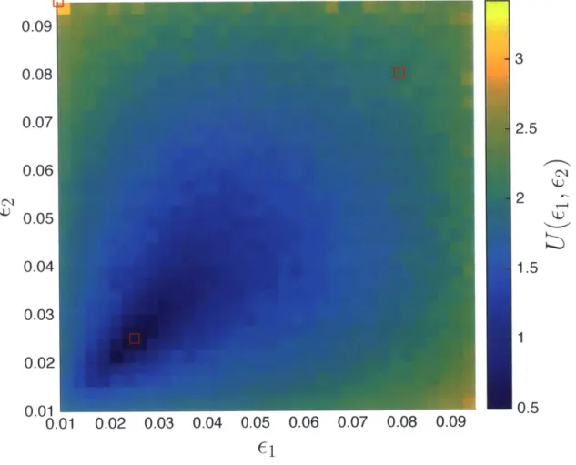
Because the ordering of the experiments is immaterial, the map of the expected information gain is symmetric about the ci = 62 line, aside from Monte Carlo esti-mation error. We draw attention to three points marked by squares in Figure 4-1. The first is at (E, 62) = (0.025,0.025), where U(ci, 62) = 0.49; it is near the minimum of the expected utility function. This point corresponds to the least useful pair of experiments. The second is at (Ei, E2) = (0.01, 0.095), with U(Ei, E2) = 2.9; it is the

maximum of the expected utility map and is expected to yield the most informative experiments. The point (E1, E2) = (0.08,0.08), where U(Ci, E2) = 2.0, lies midway between these extremes: it is expected to be more informative than the first design but less informative than the second.

To illustrate how the three (Ei, E2) pairs highlighted above yield different ex-pected utilities, we carry out the corresponding inferences of f, following the pro-cedure described in Section 3.1. To simulate each experiment, we fix f, and the desired value of 6, then generate a converged order parameter length scale A, by generating a realization of the substrate and simulating the Cahn-Hilliard

equa-0.09 - 3 0.08 0.07 _2.5 0.06 2 0.05 0.04 1.5 0.03 1 0.02 0.01 0.5 0.01 0.02 0.03 0.04 0.05 0.06 0.07 0.08 0.09

Figure 4-1: Map of expected information gain U(ci c)) iin the substrate length scale parameter fE, as a function of experimental design parameters ci and c-). The three experiments discussed in the text are marked with red squares.

tion. Given the data A,, and A,,2 corresponding to (61, 62), we evaluate the

cor-responding posterior density and calculate the actual KL divergence from posterior to prior, DKL (p(f Aoo,l:2, Ei:2)IP(f-))- The results of these three experiments are

summarized in Figure 4-2(a). As expected, the second experiment, performed at (Ei, E2) = (0.01,0.095) is the most informative, and has a large information gain of

DKL = 2.10 nats.1 The first experiment is the least informative, with a small in-formation gain of DKL = 0.99 nats. The third experiment, with _DKL = 1.44 nats,

lies in between. The actual values of DKL are different from their expected values because the expected information gains are calculated by averaging over all possible prior values of f, and all possible experimental outcomes, whereas the actual values are calculated only for particular f, and A, values, given E. However, the values of

DKL follow the same trend as their expectations.

To better understand why these experiments produce different values of the in-formation gain, Figure 4-2(b) plots Ao = EF(f,/E) as. a function of f, for c ₌ 0.01, 0.025, and 0.095. We observe that A, is not very sensitive to variations in , for c = 0.025. This explains why an experiment with (Ei, E2) = (0.025, 0.025) is not particularly informative. On the other hand, A, is sensitive to variations in , for

E = 0.095 and e = 0.01. Additionally, Ao is a decreasing function of , for 6 = 0.095,

and an increasing function for E = 0.01. The complementarity of these trends makes the experiment (Ei, E2) = (0.01, 0.095) especially useful.

We can also compare the optimal experiment to the random experiments shown in Figure 3-1(b). The information gained in the optimal experiment (DKL = 2.10 fats), with two values of 6, is comparable to the information gained from the experiment with eight randomly selected values of E (DKL = 2.29 nats). Hence by using optimal Bayesian experimental design in this example, we are able to reduce the experimental effort over a random strategy by roughly a factor of four! This reduction is especially valuable when experiments are difficult or expensive to conduct.

'A nat is a unit of information, analogous to a bit, but with a natural logarithm rather than a base two logarithm in (4.2).

102 10, 100 025 0.5 0.75 1 (a) 0.25 0.5 0.75 (b)

Figure 4-2: (a) Experiments corresponding to the three (Ei, 62) pairs indicated in Figure 4-1. The posterior densities from the three experiments are marked #1, #2, and #3. (b) A,, = EF(f,/) versus f. for E = 0.01, 0.025, 0.095.

20 18 16 14 'j 12 10 6 4 2 - -- -. I - -#2 #3 prior #1 0.095 0.025 0 .01 1n 1

Chapter 5

Conclusions and future work

In this thesis, we have demonstrated the use of Bayesian inference and Bayesian experimental design in a model film/substrate inference problem. To make inference and experimental design computationally tractable, we have used a reduced order model for the interaction between the film and the substrate. The reduced order model parameterizes the effect of the substrate on the film with a reduced set of parameters as compared to the full Cahn-Hilliard equation. The reduced order model contains both a deterministic term and a random term. The random term is necessary to model the inherent stochasticity of the substrate, the film initial condition and the

converged length scale extraction process.

We have shown that Bayesian inference can be used to infer parameters of interest with quantified uncertainty. The estimates can be improved with the inclusion of new data. The inferred value of parameters of interest, and their uncertainty is encoded in the form of a probability distribution function.

Finally, we have demonstrated the use of Bayesian experimental design in con-junction with the reduced order model to design optimal experiments. The design of the experiment is driven by an optimization of a user defined experimental utility. In this study, the experimental utility chosen maximizes the gain in information in the parameter of interest. By changing the optimality criterion, experiments can be designed with different objectives in mind.