Accelerated Bayesian experimental design for chemical kinetic models

Accelerated Bayesian Experimental Design

for Chemical Kinetic Models

MASSACHUSES

OFTECHNO

by

JUN 2 3

Xun Huan

LIBRAFS

B.A.Sc., Engineering Science, Aerospace Option (2008)

University of Toronto

Submitted to the Department of Aeronautics and Astronautics

in partial fulfillment of the requirements for the degree of

Master of Science in Aerospace Engineering

at the

MASSACHUSETTS INSTITUTE OF TECHNOLOGY

June 2010

@

Massachusetts Institute of Technology 2010. All rights reserved.

A u th or ...

...

Department of Aeronautics and Astronautics

May 21, 2010

Certified by ...

Y...

/

Youssef M. Marzouk

Assistant Professor of Aeronautics and Astronautics

Thesis Supervisor

Accepted by ...

Eytan H. Modiano

Associate Professor of Aeronautics and Astronautics

Chair, Committee on Graduate Students

Accelerated Bayesian Experimental Design

for Chemical Kinetic Models

by

Xun Huan

Submitted to the Department of Aeronautics and Astronautics on May 21, 2010, in partial fulfillment of the

requirements for the degree of Master of Science in Aerospace Engineering

Abstract

The optimal selection of experimental conditions is essential in maximizing the value of data for inference and prediction, particularly in situations where experiments are time-consuming and expensive to conduct.

A general Bayesian framework for optimal experimental design with nonlinear

simulation-based models is proposed. The formulation accounts for uncertainty in model parameters, observables, and experimental conditions. Straightforward Monte Carlo evaluation of the objective function - which reflects expected information gain (Kullback-Leibler divergence) from prior to posterior - is intractable when the like-lihood is computationally intensive. Instead, polynomial chaos expansions are intro-duced to capture the dependence of observables on model parameters and on design conditions. Under suitable regularity conditions, these expansions converge expo-nentially fast. Since both the parameter space and the design space can be high-dimensional, dimension-adaptive sparse quadrature is used to construct the polynomial expansions. Stochastic optimization methods will be used in the future to maximize the expected utility.

While this approach is broadly applicable, it is demonstrated on a chemical kinetic system with strong nonlinearities. In particular, the Arrhenius rate parameters in a combustion reaction mechanism are estimated from observations of autoignition. Results show multiple order-of-magnitude speedups in both experimental design and parameter inference.

Thesis Supervisor: Youssef M. Marzouk

Acknowledgments

When I first arrived at MIT as a graduate student, I had the littlest idea of what un-certainty quantification (UQ) is. I was very lucky to have been introduced to Professor Youssef Marzouk, and soon, he convinced me. He convinced me that not only is UQ of utter importance in engineering, its analysis is also filled with wondrous unknowns and endless possibilities. Professor Marzouk became my advisor, and more impor-tantly, he also became my friend. I remember the 7 PM meetings, "emergency" talks before quals and thesis due date, and the full day "deep-dive" discussion (with lunch of course) on a Saturday - it is these constant guidance, support, and encouragement from him throughout the two years of my Masters study that made this thesis possible.

I would like to thank the entire Aerospace Computational Design Laboratory, all the students, post-docs, faculty, and staff, for their insightful discussions from class work to research, the technical support on computational resources, and the friendships that kept me from being over-stressed. In addition, I would like to thank Professor David Darmofal for co-advising me when Professor Marzouk was away, Huafei Sun for helping revise this thesis, Masa Yano for being an awesome roommate, Laslo Diosady for the enjoyable dumpling nights, JM Modisette and Julie Andren for suspending their work to allow me to use the cluster before the thesis is due, and Hement Chaurasia and Pritesh Mody for together enduring the hardships of both the quals and thesis. But these are only a mere few of many people to be thankful for, and only a tiny count of an enormous number of things to be grateful about.

Finally, I would like to thank my parents, whose constant love and support made me who I am today. I am proud to be their son, and I wish them health and happiness.

Contents

1 Introduction

1.1 Motivation . . . . 1.2 Objective and Outline .

2 Combustion Problem

2.1 Background . . . .

2.2 Governing Equations . . . 2.3 Experimental Goals . . . . 2.4 Selection of Observables

2.5 Numerical Solution Tools

3 Bayesian Inference

3.1 Background . . . .

3.2 Prior and Likelihood . . . . 3.3 Markov Chain Monte Carlo (MCMC) . . . . .

3.3.1 Metropolis-Hastings (MH). . . . .. 3.3.2 Delayed Rejection Adaptive Metropolis

3.3.3 Numerical Examples . . . .

4 Optimal Bayesian Experimental Design

4.1 Background... . . . . . . . ..

4.1.1 Optimal Linear Experimental Design . 4.2 Optimal Nonlinear Experimental Design . . . 4.2.1 Expected Utility . . . .

4.2.2 Numerical Methods... . . . . . . . .

4.2.3 Stochastic Optimization . . . ... 4.2.4 Numerical Example.. . . . . ..

4.3 Results and Issues . . . .

5 Polynomial Chaos 5.1 Background . . . . 5.1.1 Model Reduction... . . . .. 5.1.2 Polynomial Chaos . . . . 5.2 Form ulation . . . . (DRAM)

5.3 Non-Intrusive Spectral Projection (NISP) for the Combustion Problem 5.4 Numerical Integration in High Dimension . . . .

5.4.1 Overview . . . .... 5.4.2 Monte Carlo (MC) . . . . 5.4.3 Quasi-Monte Carlo (QMC) . . . . 5.4.4 Tensor Product Quadrature (TPQ) . . 5.4.5 Sparse Quadrature (SQ) . . . . 5.4.6 Dimension-Adaptive Sparse Quadrature 5.4.7 Numerical Results... . . . ..

5.4.8 Conclusions . . . . Implementation of DASQ in NISP . . . . Detection of Polynomial Dimension Anisotropy

5.6.1 M otivation . . . . 5.6.2 Preliminary Observations . . . . 5.6.3 Detection Rule . . . . 5.6.4 Numerical Results . . . . 6 Results 6.1 PC Expansion Construction . . . . 6.2 Optimal Experimental Design... . . . .. 6.3 Validation of the Experimental Design Results

6.4 Computational Savings... . . . . . .. 7 Conclusions and Future Work

7.1 Sum m ary . . . .

7.2 Conclusions . . . .

7.3 Future W ork . . . . A Recommended Kinetic Parameter Values B Cantera Input File

Bibliography (DASQ) Using DASQ 77 77 79 80 80 81 87 93 96 97 98 98 100 101 103 105 105 107 .111 113 117 117 118 .118 121 123 129 5.5 5.6

List of Figures

2-1 Typical evolution profiles of temperature and species molar fractions in a H2-02 combustion... . . . . . . ... 24

2-2 Illustration of rg, T

H, and XH,r..-... . . . . . ... . . 26 3-1 Illustration of r0.75, the characteristic interval length of the 75% peak

values in the profile of the enthalpy release rate. . . . . 32 3-2 L2 errors of the mean estimates for multivariate Gaussians. . . . . 39

3-3 Sample fractions within the 50% and 90% regions for multivariate

Gaus-sian s. . . . . 40 3-4 The 2D Rosenbrock variant.. . . . . . . . . 41

3-5 Last 20,000 samples for the 2D Rosenbrock variant. . . . . 42

3-6 Last 20,000 samples of component x for the 2D Rosenbrock variant. . . 43

3-7 Autocorrelation functions for the 2D Rosenbrock variant. . . . . 45

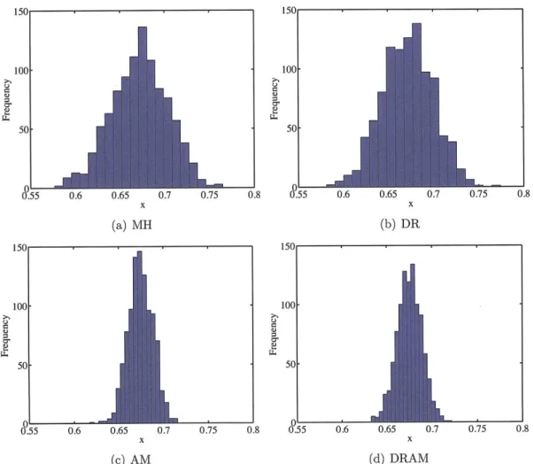
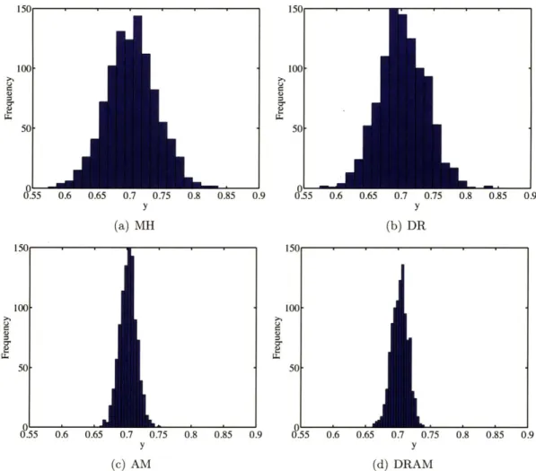
3-8 Distribution of the sample mean in x for 1000 repeated Markov chains. 46

3-9 Distribution of the sample mean in y for 1000 repeated Markov chains. 47 4-1 Expected utilities of the ID nonlinear experimental design example with

S 10-2, using different sampling techniques. The "1st Term" and

"2nd Term" are the terms from Equation 4.16... . . . . . . . . 61 4-2 Expected utilities of the ID nonlinear experimental design example

us-ing o- = 10 4,102, and 100...

. . . .

. . . ...

62

4-3

P

as a function n for Example 4.2.1. Figure (a) is where the first flip is tail, while Figure (b) is when the first flip is happens to be head. . . . . 63

4-4 Expected utilities of the ID nonlinear experimental design example us-ing a design-dependent noise level o- = |dl + 10-8.. . . . . . . 64 4-5 Expected utilities of the combustion problem with 1 design variable To,

and 2 design variables To and .. . . . . . . . . . 65 5-1 Illustration of the index sets of a 2D level 3 SQ rule. The dots are the

approximate positions of quadrature points. . . . . 83 5-2 2D sparse grid constructed using the level 5 CC rule, and the

corre-sponding tensor product grid constructed using the same ID quadrature

rule... . . . . . . . . . 86 5-3 Polynomial exactness of a 2D SQ and of its corresponding TPQ. . . . . 86

5-4 Final DASQ index sets and relative L1 error of the 2D integral using various numerical integration schemes. . . . . 94

5-5 Relative Li error of the 20D integral using various numerical integration schem es. . . . . 95 5-6 Relative L1 error of the 100D integral using various numerical

integra-tion schem es. . . . . 97 6-1 log1o of the L2 errors of the characteristic time observables. . . . 108

6-2 log1o of the L2 errors of the peak value observables... . . . .. 109

6-3 Expected utility contours of the combustion problem with 2 design

vari-ables To and

#,

using the original Cantera model (reproduced from Fig-ure 4-5(b)), and using the PC expansions with po = 4 and nquad = 1000. 110

6-4 Expected utility contours of the combustion problem with 2 design vari-ables To and

#,

using "the overkill" - PC expansions with po = 12 and nquad= 25, 000. The four designs at points A, B, C, and D are used for

validating the experimental design methodology by solving the inference problem, described in Section 6.3... ... . . .. 110 6-5 Posterior of the inference problem at the four chosen designs to validate

the experiment design methodology, constructed using "the overkill"

-PC expansions with po = 12, nquad = 25, 000. . . . 113 6-6 Posterior of the inference problem at the four chosen designs to

vali-date the experiment design methodology, constructed using the original Cantera m odel. . . . 114

6-7 Approximate computational time required for the optimal experimental

design problem. Figure (b) is the zoomed-in (note the different scale on the y axis) view . . . 115

List of Tables

2.1 19-reaction hydrogen-oxygen mechanism. Reactions involving M are three-body interactions, where M is a wild-card with different efficien-cies for different speefficien-cies. . . . . 19

2.2 Hypothetical two-reaction mechanism for Example 2.2.1. The two re-actions are Ri and R3 from the 19-reaction hydrogen-oxygen mechanism. 22

2.3 Index ordering of the reactions and species of the hypothetical 2-reaction

mechanism for Example 2.2.1. . . . . 22 2.4 Selected observables for this study. Note that dh/dt < 0 when enthalpy

is released or lost by the system. . . . . 25

3.1 Prior support of the uncertain kinetic parameters A1 and Es,3. Uniform prior is assigned. . . . . 29 3.2 Acceptance rate and number of posterior function evaluations for the

2D Rosenbrock variant... . . . . . . . 44

5.1 The Wiener-Askey polynomial chaos and their underlying random vari-ables [104] . . . . 73 5.2 "Prior" support of the design variables To and 0. Uniform prior is

assigned... ... . . . . . . ... 76 5.3 Examples of number-of-abscissas comparison between SQ and TPQ,

using C C rule. . . . . 85

5.4 Physical coordinates and positions of quadrature points in the 2D index set (2,2)... . . . . . . . . . . ... 90 5.5 Positions pi, i = 1, . -- , d of new points in ID... . . . . . . ... 90 5.6 Relationship between the number of quadrature points in a CC rule

and the maximum exact polynomial degrees. . . . 100

6.1 log1o of the L2 errors of "the overkill" - PC expansions with po = 12 and nquad = 25,000... . . . . . . . 111 6.2 Design conditions at design points A, B, C, and D. . . . 112

A.1 19-reaction hydrogen-oxygen mechanism. Reactions involving M are

three-body interactions, where M is a wild-card with different efficien-cies corresponding to different speefficien-cies. The recommended values of the kinetic parameters are shown in the last three columns [106], and their units are those described in Chapter 2. . . . 121

Chapter 1

Introduction

1.1

Motivation

Alternative fuels, such as biofuels [75] and synthetic fuels [39], are becoming increas-ingly popular in the energy market over the past years. For example, world ethanol production for transport fuel tripled between 2000 and 2007, while biodiesel ex-panded eleven-fold [10]. These fuels are excellent sources for safeguarding the volatile petroleum price and to ensure energy security, but more importantly, they carry the flexibility in promoting new and desirable properties that traditional fossil fuels might not offer.

Current knowledge about alternative fuels is relatively new. Their thermochemi-cal properties and combustion kinetics remain poorly characterized, and fundamental research in their properties is still ongoing (e.g., [21, 74]). The environments designed to produce, process, and utilize the fuels may be far from optimal. These suboptimal operating conditions lead to low efficiency and adverse emissions such as high levels of nitrogen oxides (NOx) and particulate matter (PM), both of which are not only sources of environmental and health hazard [2, 3], but are also becoming the center of political debates.

With the rapid growth of computational capability worldwide, numerical modeling has become an indispensable tool for capturing, explaining, and predicting physical

phenomena. Reliable predictions from models can lead to better designs and poli-cies for utilizing the alternative fuels, which in turn can improve their efficiency and emission rates.

One way to improve the models is to perform parameter inference. All numerical models have parameters (or constants), such as the gravitational constant in Newton's universal law of gravitation. For some models, these parameters have been experimen-tally determined or theoretically derived with great accuracy and precision; but these cases are the exception rather than the rule, since there are substantially more models where their parameters still carry significant uncertainty. For example, in combustion, many thermodynamic and kinetic parameters still have large uncertainties today [8, 9]. In an extreme example, the rate constant of a methyl elementary reaction has an un-certainty factor of 500% [82]. The accuracy of these parameters directly affect how good the models are able to represent the physical reality. Therefore, it is important to continue to refine these parameters, and reduce their uncertainty.

In order to perform inference, experimental data need to be used, but not all data are created equal - while some data can be very helpful in reducing the parameters' uncertainties, other data may not be useful at all. Since experiments, especially in the combustion field, are expensive, time-consuming, and delicate to perform, it is thus crucial to design experiments that yield data of the highest quality. This process is called optimal experimental design, and shall be the centerpiece of this thesis. A Bayesian approach to the optimal experimental design shall be undertaken, which is able to account for uncertainties in model parameters, observables, and experimental conditions.

Further background information and literature review are presented in each of the chapters accordingly, as the thesis progresses.

1.2

Objective and Outline

The primary objective of this thesis is to formulate a mathematical framework of computing the optimal experimental designs for nonlinear models under a Bayesian setting. In particular, this framework is demonstrated on a challenging chemical com-bustion system to illustrate its effectiveness and practicality. However, this nonlinear optimal experimental design framework is very general, and can be applied to many other models in a wide range of applications.

This thesis is outlined as follows. The physical problem of interest, the combus-tion problem, is introduced in Chapter 2. Its understanding is essential in establishing the goals of the physical experiment. Chapter 3 then provides the tools necessary to achieve the experimental goals, and these tools also create the foundation on how to quantify the value of an experiment. With the aid of concepts from information the-ory, the goodness indicator is developed in Chapter 4. This subsequently enables the optimization of experimental designs, and the experimental results from the optimal design would allow the experimenter to best achieve his or her experimental goals. However, this nonlinear optimal experimental design framework is shown to be too expensive to be practical, and its acceleration through model reduction is necessary. Chapter 5 presents one such reduction method, by forming polynomial chaos expan-sions for random variables. Combining all the tools, the experimental design problem for the combustion system is solved in an accelerated manner, and the results are pre-sented in Chapter 6. Finally, the thesis ends with a summary, and some conclusions and future work in Chapter 7.

Chapter 2

Combustion Problem

Each experiment is performed with some purposes or goals. These goals are important

i

1. determining which experimental states should be observed; and

2. quantifying the goodness of an experiment, which subsequently allows the opti-mization of experimental designs.

In order to perform these tasks, it is essential to have a good understanding of the physical problem relevant to the experiment. The physics, along with the first task, are described in this chapter; the second task is discussed in Chapter 4.

2.1

Background

The hydrogen-oxygen (H2-0 2) combustion is chosen as the physical problem of interest.

Better understanding of this simple yet representative combustion paves the path to better understanding of the combustion of larger molecules. In fact, H2-02 has

already been studied extensively in the history of combustion [24, 98, 99, 106], and is currently one of the best-understood mechanisms, thus conveniently providing ample data for validation. The so-called "hydrogen economy" [68], or even simply blending hydrogen with traditional fuels (e.g., [53]), has also received considerable attention

as the cleaner future replacement to the current "hydrocarbon economy", further motivating continued research in the fields related to H2-0 2.

The combustion of a fuel is a very complicated process, involving the time evolu-tion of numerous chemical species. A spectrum of mechanisms have been developed to describe the H2-0 2 combustion. On one extreme, a one-step global mechanism

resembles a "black-box" type of approach. It captures the development of the major reactants and products, but does not reflect what is really happening with the interme-diate species (i.e., the detailed kinetics). Also, the global kinetic relation often relies on curve-fitting of experimental data, leading to non-integral reaction orders which can be non-intuitive. On the other extreme, a very detailed mechanism composed of elementary reactions is able to reveal comprehensive interactions among the interme-diate species. The tradeoff, however, is its high computational cost and complexity. As a result, it is important to find the simplest mechanism that captures the reaction behaviour that is relevant to the experimental goals.

This study has taken an in-between approach, by choosing a mechanism of interme-diate complexity - a 19-reaction mechanism proposed in [106], which is reproduced in Table 2.1 (a more extensive table containing the recommended values of kinetic parameters can be found in Appendix A). A detailed discussion of the roles of each reaction can also be found in [106].

For demonstration purposes, constant pressure, adiabatic, and no-transport (i.e., homogeneous) conditions are considered. To some extent, these conditions can imi-tate the conditions of shock tube experiments for a short period of time right after the passing of the reflection wave (in some cases, constant-volume and isothermal conditions may be more appropriate). This can be of significance because shock tube experiments are one of the standard experimental methods for analyzing chemical kinetic properties [18, 19] (some other alternatives include static-, stirred-, and flow-reactors, as well as rapid compression machines and even premixed flames [44]). In an engineering example, jet engines burn fuel in the combustor at near constant pressure condition [46]. The methodology to be developed in this thesis can be easily applied

to various different, more complex reaction conditions, and has great potential in a wide range of applications.

Reaction No. R1 R2 R3 R4 R5 R6 R7 R8

R9

RIO R11 B12 R13 R14 R15 R16 R17 R18 R19 Elementary Reaction

H+0

₂

O

+

H2 H2

+OH

OH + OH H₂

+ M

O+OA+M O+H-+ M H + OH + AM H + 02 + M H02

+ H

HO

2

+ H

H02

+ O

H02

+ OH

HO

₂

+

HO2 H202 +

M

H202

+ H

H202

+ H

H202

+ O

H202

+ OH

Kz~ O+OH H+OH H2 0+H

O +

H20 H±H+M 0 2

+ M

OH + M H20

+ M

H02

_{+ M}

H2 + 02 OH + OH 02

+ OH

H20

+

0 2 H202 + 02 OH+-OH+M H20

+ OH

HO2

+

H2

OH +

HO₂ HO2

+

H20

Table 2.1: 19-reaction hydrogen-oxygen mechanism. Reactions involving M are three-body interactions, where Al is a wild-card with different efficiencies for different species.

2.2

Governing Equations

The state of the chemical system can be completely described by the species mass

frac-tions Y [dimensionless],

j

= 1, .. . , n. (where n, is the total number of species), and

the system temperature T [K]; they shall be referred to as the state variables. Given the assumed conditions described earlier (constant pressure, adiabatic, no transport),

the system is governed by the following set of ordinary-differential equations (ODEs): dY gW. (2.1)

dt

p

dT 1fs - - ZhwnW _(2.2) dt _Ppn= Initial Conditions = I o'

V

(2.3)

T

o = To

0

where LOj [kmol -m-3

s

-1] is the molar production rate of the jth species, W [kg - kmol-1]

is the molecular weight of the jth species, p [kg m m-3] is the mixture density, c, [J - _{- kg-1] is the mixture specific heat capacity under constant pressure, and h"} [J kg 1] is the specific enthalpy of the nth species. More specifically, the molar

production rate is defined as d [ Xj |

j 24

COj = dt = (v rn v ) kf,,m 11 [Xn]"" kr,mn f [Xn]"1 ,Vj 24

m=1 n=1

where [Xj] [kmol m-3] is the molar concentration of the jth species, nr is the total number of reactions, and v and v [dimensionless] are the stoichiometric coefficients on the reactant and product sides of the equation, respectively, for the nth species in the mth reaction.

The forward and reverse reaction rate constants of the mth reaction, denoted

by kf,m

[(m3

- kmol-

)

" -

sI

_ and kr,m [(m3 - kmol-±)Z * -s-

11

re-spectively, are assumed to have the modified Arrhenius form:

kf,m = AmTb- exp ( 4 n) (2.5)

kr, - kf,mrn kfrn (2.6)

where Am

[(m3

kmol 1

)

-

s-1 -K-b" is the pre-exponential factor, bm [dimensionless] is the exponent of the temperature dependence, Ea,m [J - kmol 1] is the activation energy (Am, b.m, and Ea,m are collectively called the kinetic parameters of reaction m), R, = 8314.472 [J kmol' - K-] is the universal gas constant, Kc,,

(3

-

kmol-1) _ is the equilibrium constant, and AG'm

[J

kmol

is the change in Gibbs free energy at standard pressure (101,325 Pa) and temperature

T.

The initial conditions of the ODEs are described by Equation 2.3, where Y,o and To are the initial species mass fractions and temperature, respectively. In most cases, the initial mass fractions of all species are zero except for H2 and 02. This leads to a compact, equivalent method to express Y,o, using the equivalence ratio

#

[dimen-sionless], which is an indication of whether the fuel-oxidizer mixture is rich, lean, or stoichiometric:

(Y0 2

/YH2)stoic

(X02

/XI

2)stoic

(2.

(Yo2/YH2) (Xo2/XH2)

where the subscript "stoic" refers to the stoichiometric ratios, and Xj [dimensionless] is the molar fraction of the jth species, related to the mass fraction through

Wj Y (2.8)

Xj W J("' = Yn / Wn

Often, the xj's are used in place of the Yj's as the state variables, and this is adopted for the rest of the thesis.

Finally, perfect gas mixture is typically assumed, closing the system with the fol-lowing equation of state:

p = (2.9)

RT E",( Yn/W/n'

where p [Pa] is the (assumed constant) pressure. Note that different reaction conditions would lead to different variations of the governing equations.

Example 2.2.1 demonstrates how Equation 2.4 can be formed through a concrete case.

Example 2.2.1. Two-Reaction Mechanism

Consider a hypothetical two-reaction mechanism described in Table 2.2, which is

simply constructed by reactions RI and R3 from the 19-reaction H2-0 2 mechanism described in Table 2.1. The reactions and species of this mechanism are arbitrarily ordered according to Table 2.3. Consequently, the stoichiometric coefficient matrices are

, 1 0 0 0 1 0 ,, 0 0 0 1 0 1

v0n

0v,

1.

(2.10)

0 1 0 0 0 1 0 0 1 0 1 0

Equation 2.1 for

j

= 6 (i.e., species OH), for example, can be formed as

d[X6] d[OH]

- dt dt

=

(1

-

0) (kf,1 [X1] [X5] - kr,, [X4] [X6]) +

(0 - 1) (kf,2 [X2] [X6] - kr,2 [X3] [X5])

= kf,i [02] [H] - kr,1 [0] [OH] - kf,2 [H2] [OH] + kr,2 [H20] [H] . (2.11)

Reaction No. Elementary Reaction

RI H+0 2 < 0 +OH

R3 H2

+OH

M

H20+

H

Table 2.2: Hypothetical two-reaction mechanism for Example 2.2.1. The two reactions are RI and R3 from the 19-reaction hydrogen-oxygen mechanism.

m 1 2 n 1 2 3 4 5 6

Reaction RI R3 Species 02 H2 H20 0 H OH

Table 2.3: Index ordering of the reactions and species of the hypothetical 2-reaction mechanism for Example 2.2.1.

2.3

Experimental Goals

Experiments can be designed and performed with different goals. For example, while one experiment may be used to infer certain parameters in the model, a different experiment can be more suited to predict the future behaviour of the system. The experimental goals will ultimately dictate what outputs should be observed or com-puted, and what the criteria are for a good experiment. The former is discussed in the next section (Section 2.4) while the latter is to be discussed later on (Chapter 4).

In this study, the experimental goals are to infer the values of (some or all of) the kinetic parameters (AM, bm, and E,m) of a subset of elementary reactions described in Table 2.1.

In the future, thermodynamic and transport parameters may also be explored.

2.4

Selection of Observables

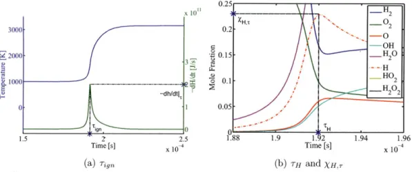
Typical evolution profiles of the state variables are shown in Figure 2-1. In the fol-lowing discussions, the initial conditions of the system shall be assumed to cause an ignition (explosion), unless otherwise specified.

The most complete and detailed set of observables of the system is simply the state variables as a function of time. To handle this numerically, one could, for ex-ample, discretize the time domain. However, too few discretization points would fail to capture the state behaviour, while too many discretization points would lead to an impractically high dimension of the observable vector. Also, as to be discussed at the end of Section 5.2, time-discretized states would be difficult to capture using polynomial chaos expansions. Therefore, one should transform the state variables to some new observables that in some sense compress the information, while retaining the information relevant to the experimental goals (analogous to sufficient statistics from information theory).

Given the experimental goals of inferring the kinetic parameter values, the observ-ables must be able to reflect the variations in the kinetic parameters. For example,

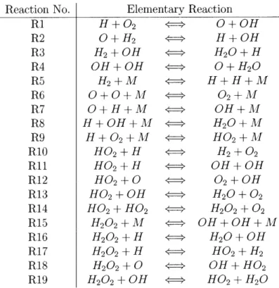
3500 H 3000 0.6 -0 0.5- _OH Z2500 C ₀ _HO 2 0.4 H 2000 _HO 1500 0.3 _HO02 202 E1500- 0.2-1000 _0.1 500 0 0 1 2 3 4 5 0 1 2 3 4 5 Time [s] X 10-4 Time [s] x 104

(a) Temperature (b) Species molar fractions Figure 2-1: Typical evolution profiles of temperature and species molar

frac-tions in a H2-02 combustion.

temperature and species molar fractions at steady-state or equilibrium would not be able to reflect the kinetics of the system, although they would be good candidates for inferring thermodynamic parameter values. Another desirable property of the observ-ables is that they are common and easy to measure in real experiments. For example, ignition delay is a very common and relatively easily measurable output in kinetics-related experiments, with ample data available in the literature. On the other hand, a characteristic time in which [H₂0] reaches 75% of its equilibrium value would be

more difficult to pinpoint, and almost never reported in the literature.

Taking the above factors into consideration, observables listed in Table 2.4 are selected for this study. The first 5 are characteristic times related to peak values, and the last 5 are the corresponding peak values. Note that dh/dt < 0 when enthalpy is released or lost by the system (i.e., exothermic). The species chosen for the observables are radical species (reactive due to unpaired electrons), which possess a peak in the mole fraction profiles (or a double peak in the case of H202). The peaks are caused by the following phenomenon. Prior to the ignition, radicals slowly accumulate in a pool

by the chain-initiating reactions. After surpassing some threshold, they activate the

chain-branching reactions, which further produce radicals very rapidly, leading to the

-ignition of the system. Soon after, reverse reactions balance the forward radical pro-ductions, while the chain-terminating reactions finally convert them to stable forms. Examples of ig, TH, Lh . and XH,, are shown in Figure 2-2. The time of the peak enthalpy release rate approximately matches the point when temperature rises most rapidly, as expected. As to be discussed later on in the thesis, the ln of the charac-teristic times shall be used in the actual implementation, that is, ln r's instead of T's. This does not make any difference in the formulations except that the constructions of the polynomial chaos expansions in Chapter 5 would be for approximating the ln T's

instead of the r's.

Observable Explanation

T_{ign Ignition delay, defined as the time of peak enthalpy release rate.} TO Characteristic time in which peak XO occurs.

T_{H Characteristic time in which peak XH occurs.} rHO2 Characteristic time in which peak XHO2 occurs.

TH202 Characteristic time in which peak XH202 occurs.

dt 1T Peak value of enthalpy release rate.

XO,r Peak value of XO.

XH,r Peak value of XH.

XHO2,T Peak value of XHO2'

XH202,T Peak value of XH202 '

Table 2.4: Selected observables for this study. Note that dh/dt < 0 when enthalpy is released or lost by the system.

2.5

Numerical Solution Tools

The governing equations are solved using Cantera version 1.7.0 [1, 33], which is an open-source chemical kinetics software. The Cantera input file used is presented in Appendix B. In particular, Cantera solves the system of ODEs with the help of

CVODE [16], a suite of nonlinear differential algebraic equation solvers that solves stiff ODE systems implicitly, using the backward differentiation formulas. The validity and

performance of the software are not assessed in this study, but extensive benchmark testings have been done by their developers [4]. One may view the software simply as

x 10'1 0~ HO 2000 -0.15 2 3 ---H HO 0 1000 0.1 2 -dh/dtl 0 1 0.05 Ig. 0 0 -1.5 2 2.5 1.88 1.9 1.92 1.94 1.96 Time [s] X 10-4 Time [s] X 10

(a) Tin _(b) TH and XH.,

Figure 2-2: Illustration of Tgn, TH, and XH,T.

third-party tools used in this study.

It has been occasionally encountered under some conditions that Cantera would fail. This may be caused by the fact that Cantera enforces the constant pressure condition via a high-gain controller for adjusting the volume, which can sometimes cause the system to "overreact", leading to negative volumes. Through some experi-mentation, most of these problems can be solved with "engineering solutions" such as relaxing the tolerances of the CVODE time integrator, and perturbing the final time to be integrated to.

Chapter 3

Bayesian Inference

The experimental goals have been defined in Section 2.3, which are to infer the kinetic parameter values of the mechanism reactions. These goals can then be used to quan-tify the goodness of an experimental design. However, before that can be done, the method of solving this inference problem needs to be introduced, as the indicator of goodness typically requires solving the inference problem itself. Furthermore, solving the inference problem is necessary in validating the final design optimization results.

3.1

Background

Parameter inference can be broadly divided into two schools of thought - Bayesian and non-Bayesian. The former treats the unknown as a random variable, incorporating both the experimenter's prior knowledge and belief, as well as observed data, via Bayes' theorem. The latter models the observed data as being parameterized by the unknown variable, which has a deterministic, albeit unknown, value. While both approaches have been studied extensively, there does not appear to be a clear superior method; rather, one method can be a more suitable choice depending on the problem structure. Some discussions about the advantages and disadvantages of the two approaches can

be found in, for example, [25] and [92].

natural structure for sequential parameter inference as well as sequential experimental design. An introduction to Bayesian analysis can be found in [84], while a more theoretical discussion can be found in [45].

Let (Q,

F,

_{P) be a probability space, where Q is the sample space, F is the --field,} and P is the probability measure. Let the vector of random variables 6: Q -+ RiO be the uncertain parameters of interest whose values are to be inferred, y {y}U be the set of nmeas data, where Y, : Q -+ R ' is one particular datum, and d E Rnd be the experimental conditions. Here, no is the number of uncertain parameters, ny is the number of observable categories (e.g., Table 2.4 results in ny=10), and nd is the number of design variables.

At the heart of the Bayesian inference framework is, of course, Bayes' theorem. It can be expressed in this context as

p (y|6, d) p(6 d)

p (01 y,

d)

=

(3.1)

p (yl d)

where p (61 d) is the prior probability density function (PDF), p (y|

6,

d) is the

likeli-hood PDF, p (61 y, d) is the posterior PDF, and p (yl d) is the evidence PDF.

More-over, the common assumption that the prior knowledge is independent of the experi-mental design can be made, simplifying p (61 d) = p (6). Upon obtaining the posterior

PDF, point or interval estimates may also be constructed.

3.2

Prior and Likelihood

For the purpose of demonstration, the unknown kinetic parameters are chosen to be A1 and Ea,3 (i.e., the pre-exponential factor of reaction RI and the activation energy of reaction R3), while all other kinetic parameters are set to their recommended values, tabulated in Appendix A. In particular, instead of controlling A1 directly, a transformation of

A

1 = ln (A1

/A*)

(where A* is the recommended value of A1) shall be used instead, which is useful in constraining A1 to positive values only. Extension to additional parameters is easily generalizable.

The support of the parameter prior usually reflects constraints of physical admis-sibility, experimental limits, or regions of interest. Ranges for kinetic parameters, however, are not as intuitive as more familiar variables such as temperature. There-fore, some preliminary tests have been performed to determine "interesting regions" of these parameters using the error models constructed in the next section. More specif-ically, these regions are those having relatively large posterior values. Furthermore, a uniform prior is assigned across the support adhering to the principles of indifference and maximum entropy [41]. The uniform prior is also the non-informative Jeffreys prior [42] using the Gaussian likelihood models to be introduced shortly. The prior support is summarized in Table 3.1.

Parameter Lower Bound Upper Bound

A1

-0.05 0.05

Ea,3 0 2.7196 x 107

Table 3.1: Prior support of the uncertain kinetic parameters

A

1 and Ea,3. Uniform prior is assigned.

In constructing the likelihood, an additive error model is assumed for the observ-ables

Y; (0, d) = g (0, d) + c (d), V1, (3.2)

where g (0, d) is the output from the comfputational model (i.e., Cantera), and F (d) =

(ei

(d) , - - -, (d)) is the additive error. Furthermore, the error shall be assumed to

be i.i.d. zero-mean Gaussians ci ~ A(0, of (d)). This independence property

conve-niently makes the different entries in a datum vector to be independent conditioned on the parameters

0.

Additionally, data measurements (i.e., the different yj's) can be

reasonably assumed to be independence conditioned on 6, and hence fmeas p(yj6,d) = p(y 1

l0,d)

nmeas fy = fJ p (yl, 1 0, d) 1=1 i=1 1 (e- g (0, d))2 -

111

exp

2.

(3.3)

=1

i=1

v

2o

The o 's are allowed to be a function of the design variables (but not of uncertain parameters). The reason for this choice is that the observables in the combustion problem can vary over orders of magnitude when the design variables are changed within reasonable ranges - for example, such an H2-02 combustion at T = 900 K has Tg, on the order of 10-1 seconds, while at T = 1000 K, 10-3 seconds. Thus having the same error "width" at the two design conditions with such different observable values would seem unrealistic. For example, measurement error magnitudes generally increase with the measurement magnitudes. On the other hand, preliminary testings indicate that the observables are much less sensitive to the unknown parameters within the prior support set earlier, and thus the 0 dependence is not included in the oi's. Its inclusion, if desired, would be trivial to implement. Additionally, because of the large variations of the characteristic time observables, instead of directly using the T's in the implementation, their natural log values, ln T's, are used for the rest of this thesis. However, the c's are still Gaussian with respect to the non-log values. Thus, the only difference this would make is that, as to be introduced in Chapter 5, the polynomial chaos expansions would approximate the ln T'S instead of the T'S.

The ojs are determined as follows. At the desired design conditions d, a simulation at the recommended parameter values is performed to obtain the nominal observable values. For the peak-value observables ( T, X0,T, XH,T, XHO2,T, and XH202,), USs are

simply chosen to be 10% of the nominal observable values. For the characteristic-time observables (rig,, TO, TH, THO2, and TH0 2), a common value of o shall be used (because

all five of these characteristic times typically have very similar magnitudes), which is represented by a linear model:

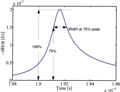
a = a + bTo. 75 (3.4)

TO7 5 is the characteristic interval length of the 75% peak values in the profile of the

enthalpy release rate - this is illustrated in Figure 3-1. The purpose of a is to establish some minimum level of error, reflecting the resolution limit of timing technology. The purpose of b is to represent an assumed linear dependence on some width measure of a peak. The rationale is that pinpointing the maximum of a flatter peak would be experimentally more challenging, since the measurement error on the magnitude of the quantity would be more significant compared to the variation of the quantity across the peak - in other words, similar values would be more difficult to differentiate. This might be counter-intuitive since one often expects a very acute peak to be harder to detect. However, the detection issue is a matter of sensor resolution, which is reflected

by the constant term a, not by b. For this study, a = 10- seconds is a realistic choice, while b = 10 appears to work well after some experimenting.

3.3

Markov Chain Monte Carlo (MCMC)

In this section, all data and analysis are assumed to be from a fixed design condition,

d. With this assumption in mind, conditioning of d in PDFs shall be dropped in the

notation for simplicity.

In general, the PDF of the posterior does not have an analytical form. The obvious method to construct the posterior is to simply form a grid in

E

(where

E

is the support of p (6)), and evaluate the posterior values at the grid points. While this can be done if

E

is of very low dimensions, it becomes impractical for more than, say, two dimensions, as the number of grid points grows exponentially with the number of dimensions. Instead, a more economical method is to generate independent samples from the posterior PDF (e.g., via Monte Carlo). However, since the posterior generally

x 1011

0.5

0

1.88 1.9 1.92 1.94 1.96

Time [s] X 10

Figure 3-1: Illustration of T0.75, the characteristic interval length of the 75%

peak values in the profile of the enthalpy release rate.

does not have an analytic form, direct sampling from it would be difficult. Even if it does have some analytic form, the inverse-cumulative density function (CDF) sampling method cannot be used in multiple dimensions. The most robust method is perhaps the acceptance-rejection method, but that would almost always be very inefficient.

Markov chain Monte Carlo (MCMC) offers a solution, by constructing a Markov chain whose target distribution is the posterior, while trading off the independence of the samples. Nonetheless, a well-tuned MCMC can offer samples with very low correlation. The main advantage of MCMC is that the target distribution can be constructed solely based on point-wise evaluations of the unnormalized posterior. The resulting samples can then be used to either visually present the posterior or marginal posteriors, or to approximate expectations with respect to the posterior

with the Monte Carlo estimates

ffn l f (6(t), (3.6)

nMt=1

where nm is the number of MCMC samples, and 6()'s are the MCMC samples. For

example, the popular minimum mean square error (MMSE) estimator is simply the mean of the posterior, while the corresponding Bayes risk is the posterior variance.

MCMC is supported by a strong theoretical foundation, and also requires finesse

in its implementation - a well-implemented MCMC is an art itself. Awareness of its numerous variations, diagnostics, tricks, and caveats is essential in creating an effective

MCMC algorithm. This thesis does not attempt to survey the enormous number of

theoretical and practical topics of MCMC, but rather, the reader is referred to [5] for a brief review, and [31, 78] for detailed discussions.

3.3.1

Metropolis-Hastings (MH)

One simple and popular variation of MCMC is the Metropolis-Hastings (MH) algo-rithm, first proposed by Metropolis et al. [61], and later generalized by Hastings [38]. The algorithm is outlined in Algorithm 1.

Additionally, if the proposal is symmetric (i.e., q (e

(t)

=) q (0' 0(t))), then

the acceptance probability in Equation 3.7 reduces to

a' (0, ') =pmin 1 p (6'l y) (3.8)

which is known as the Metropolis algorithm [61].

3.3.2

Delayed Rejection Adaptive Metropolis (DRAM)

Two useful improvements to MH are the concepts of delayed rejection (DR) [34, 62] and

Algorithm 1: Metropolis-Hastings algorithm. Initialize 0(t) where t = 1;

while t < nM do

Sample candidate state

0'

from proposal PDF q (.| 0(o);

Sample U ~ U (0, 1); Compute

a(6w, 6') = min 1, Oly M0 . (3.7)

p-

FOt y) q ( 'l OGt

if U < a (O

of')

then 0t+ = 0' (accept); else 0 (t+1) _ 0(t) (reject); end t = t +1; end Delayed Rejection (DR)

The idea behind DR [34, 62] is that, if a proposed candidate in MH is to be rejected, instead of rejecting it right away, a second (or even higher) stage proposal is induced. The acceptance probability in the higher stages are computed such that the reversibil-ity of the Markov chain is preserved. This multi-stage strategy can allow different proposals to be mixed, for example, with the first stage proposal to have a large proposal "width" to detect potential multi-modality, while the higher stages to have smaller "widths" to more efficiently explore local modes. Additionally, it has been shown [93] that DR improves MH algorithm in the Peskun sense [73], by uniformly reducing its asymptotic variance.

algo-p (-6'| y( ) q 0(t) = min

1,_{p 00 y) q (0'\10}

= min 1, N

and the second stage has an acceptance probability

a2

(OM,

0/'10)

= min

~~

1, (2y) q1 (' 1\0') q2 06

0'1,'2- 0 1c (O'2, Of,)]

p

(

t

y)

q1

(

'1\0(t))

q2

(0

1

O(t)

,1

[ -

a

₁

(O(t),'1]

= min 1 . (3.10)

In general, the ith stage has an acceptance probability

(

r ( O ' y ) 1 ( O 'i - | ) 2 ( 0 - | I - , s .i (I)0 , ,

= min 1, i- 0 )q O' 2 '-1 1 . i(0t -0 -- '

-(8 )y)qi (0'10(t))q2 ( 010t), 0/)--qi (01J00,0",---,'01_1

[1 - a1 (0', 0'_1) [1 - a2 (0', 0'_1, 0'-2] .[ - I (00, - 01)]

[1 ),0)] ai(8 i a2(80, 1,0) - - [ - i-1 (0), 01, - - 01

= m in 1 (3.11)

Upon reaching the ith stage, all previous stages must have led to rejection, and hence N3 < D. for

j=1,*-,

i-1. Thus, a3 (6t)0, ., 0'i, ) - Nj/D, which leads to a

convenient recursive formula

Di = qi '

l

00(t), 0'), - - - , 1). (3.12)

Since each stage independently preserves the reversibility of the Markov chain, DR may be terminated after any finite number of stages. An alternative is to terminate with probability PDR at each stage. Upon termination, the original state 0(t) is retained as in a rejection case.

rithm

i

0(t),

0')

(3.9)

Adaptive Metropolis (AM)

The tuning of the proposal "width" and "orientation" in MH is a tedious, but necessary task. It requires trial-and-error, and the resulting optimal parameters are different for different problems. For example, too large of a width would lead to high rejection probability, causing slow movement of the chain and thus poor mixing; too small of a width would lead to high acceptance probability, but each accepted state would be very close to the previous state, again leading to slow mixing. An automated way of tuning is desirable.

There exists numerous adaptation algorithms that are based on past samples in the chain history (e.g., [79, 94]). However, such alterations often destroy the Markov property of the chain, and hence the usual MCMC convergence results are no longer valid. This problem can be avoided if the adaptation is not performed constantly (e.g., only during a burn in period to tune the proposal parameters), or else the algorithm's ergodicity has to be proven separately. The AM algorithm by Haario et al. is an example of the latter, and is introduced below.

A multivariate Gaussian proposal centered at the current state, q (o'i6 ~(t)

.N

(o(1,

E), is assumed, with the proposal width and orientation reflected through its

covariance matrix E. Haario et al. [36] first proposed the Adaptive Proposal algorithm, where it updates E with the sample covariance matrix using samples in a fixed window of history. However, this algorithm was shown to be non-ergodic. Improvements are then made by Haario et al. [37] to introduce the AM algorithm, which uses all the past samples in history to form the sample covariance matrix, and is proven to be ergodic. This algorithm is described in detail below.

Let E1 be some initial proposal covariance matrix set by the user, the subsequent update at iteration t is then

E ,

_{t <}

_nA

nA is the iteration number in which the adaptive covariance matrix replaces the initial covariance matrix. The reason for this delay is that some initial samples are required for the sample covariance to have some significance, but of course the larger nA is, the longer before AM starts to have its effect. At the same time, E1 cannot be totally unreasonable - for example, if all samples before nA are rejected, the sample covariance would be singular, and does not give much useful information in adapting E(). Id is the d-dimensional identity matrix, and E > 0 is a small perturbation that

makes sure E(t) is non-singular. Sd _{is a scaling factor for the proposal. For example,}

sd = 2.42

_/d

_{is the optimal value for Gaussian target distributions [26].}

The sample covariance needs not be re-computed from all samples at each iteration, but can be simply updated through the formula

Cov (6(1 ---. '(t)) t - 1 ( (t) (6(t)) - to(t) ( (t) , (3.14) where ()

I

_ t -_l( 1) I 6 Y(t) - - _{_ + 6 (3.15)} i=1

is the sample mean, and can be easily updated with the recursive formula above. Substituting Equations 3.14 and 3.15 into Equation 3.13 yields the recursive formula

(t - 2) E + dt) (t - 1) 0(t- - (t) M - 0(t) 0(t)T + El . (3.16)

(t - 1) t - 1 ( (

One may also choose to update E every n iterations instead of every iteration.

Combining DR and AM

There are various ways to combine DR and AM [35]. The most direct method, as adopted by this study, is as follows.

* Perform DR at each iteration as described. At the ith rejection stage, one can simply set qi = yqi_,, where -y is a scaling factor. The magnitude of -y reflects

how rapidly the covariance resizes upon each rejection. Experience shows that choosing a slightly larger Ei and setting -y E (0, 1) works well (e.g., y = 0.1). * At the end of an iteration, only one sample would emerge - either the same

sample as the previous iteration (i.e., rejected through all stages before termi-nating DR), or a sample accepted at some stage. That sample is used to update E(') using the AM method described.

3.3.3

Numerical Examples

Two simple test cases are presented to compare the performance between MH, DR, AM, and DRAM. The first case involves a series of multivariate Gaussians, which are relative easy target distributions for MCMC; the second case involves a variant of the Rosenbrock function, which has a very nonlinear, banana-shaped peak that provides a more difficult challenge to these algorithms. The examples are similar to those found in [35], but not exactly the same.

Multivariate Gaussians

In this test case, correlated zero-mean multivariate Gaussians

.A

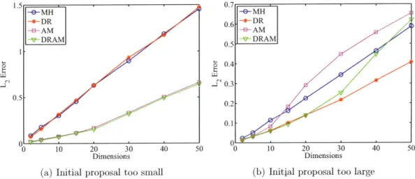
(0, Etr) of different dimensions are used as the target distributions. In order for the comparisons across dimensions to be meaningful, Eta, for each dimension is randomly generated, while fixing the condition number at 10. The initial proposal covariance matrices, the E1's,

are taken to be proportional to the Etr's. Two situations are considered:

1. the proposal is too small, by setting E1 O=OlsdEtar; and

2. the proposal is too large, by setting Ei 4

sdEtr.

In other words, the proposal covariances are well-oriented, but not well-scaled. The initial position is taken to be (-1, - --, -1), away from the Gaussian mean. For DR, a maximum of 2 stages are allowed (i.e., a total of 2 levels of proposals), with 7y = 0.1.

with no burn in. At each dimension, statistics are averaged over 100 independent

MCMC runs.

The L2 errors of the sample means are computed. The results are shown in Fig-ure 3-2. The errors grow as dimension grows, due to the fixed length of the Markov chains. More interestingly, the AM and DRAM outperform MH and DR when E1 is too small, while all four algorithms have similar performance when Ei is too large. The reason for this observation is that, since DR only scales down the proposal covariance, DR has no effect when E1 is already too small.

1.5 0.7 -0-MH M -*-DR 0.6 -*-DR -B-AM -e-AM SDRAM 0.5 -DRAM 0.4 .T0.3 0.5 0.2 0.1 00 10 20 30 40 50 00 10 20 30 40 50 Dimensions Dimensions

(a) Initial proposal too small (b) Initial proposal too large

Figure 3-2: L2 errors of the mean estimates for multivariate Gaussians.

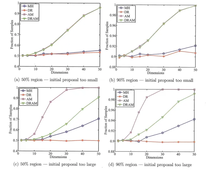
Another analysis is to compute the fractions of sample points that fall within the

50% and 90% credible regions centered around the mean of the Gaussians (i.e., the

origin). In a 2D contour, such region is simply an ellipse centered around the origin. The results are shown in Figure 3-3. In all cases, the AM and DRAM algorithms tend to oversample from the central regions of the Gaussians, especially as the number of dimensions increases. However, MH and DR are able to resist such phenomenon. This indicates a potential drawback in AM, that a too well-tuned proposal may induce oversampling in the high probability regions. One possible method to alleviate this problem in high dimensions is to choose a larger nA or to adapt less frequently (e.g., adapt every ni iterations).

(a) 50% region - initial proposal too small

(c) 50% region

20 30 40

Dimensions

initial proposal too large _{(d) 90% region}

20 30 40

Dimensions

initial proposal too large

Figure 3-3: Sample fractions within the 50% and 90% regions for multivariate Gaussians.

Rosenbrock Variant

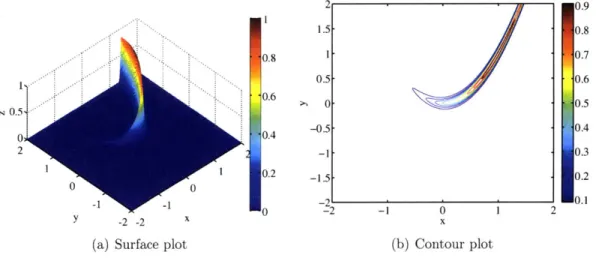
Let the target (unnormalized) PDF of the MCMC be the following variant of the 2D Rosenbrock function for (x, y) E [-2,2] x [-2, 2]:

f

(x, y) = exp

{

- [(1 -x)2 + 100 (y -x2)2] .

The original Rosenbrock function is often used to test optimization algorithms, and it has a sharp banana-shaped valley which is near-flat along the bottom of the valley.

(3.17)

In the variant, the negative inside the exponential "flips" the valley, turning it into a peak. The exponential ensures the function to be positive, and at the same time making the peak even sharper. The variant function is shown in Figure 3-4.

2 0.9 1.5 0.8 0.8 1 0.7 0.5 0.6 '0.60 0 0.-0.5 -0.5 -. W 0.4 2 -1 0.3 2 -0.2 0.1 0

~ ~

0

~

71

(a) Surface plot (b) Contour plot

Figure 3-4: The 2D Rosenbrock variant.

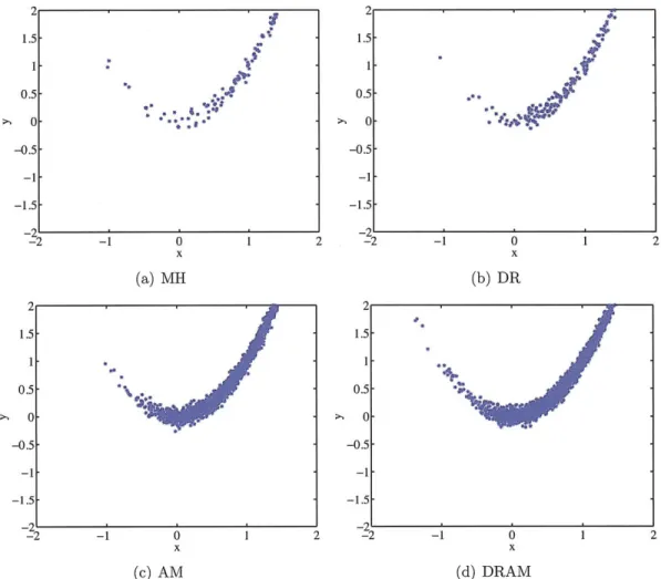
The MH, DR, AM, DRAM algorithms are run for 100,000 iterations, with a burn in of 1000 iterations. The initial proposal covariance matrix is E, diag (10.0, 10.0) (which is much "wider" than the "thickness" of the banana peak, or even the prior support), and the initial position is (-2, -2). For DR, a maximum of 2 stages are allowed (i.e., a total of 2 levels of proposals), with -y =0.1. For AM, 'nA =10 is

selected.

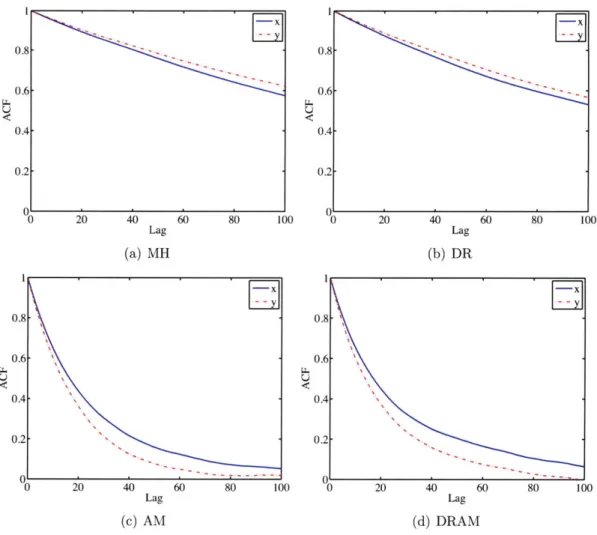
The last 20,000 samples from the algorithms are plotted in Figure 3-5, all of which resemble the banana-shaped peak from Figure 3-4. However, the plots for MH and DR appear less well mixed, indicating more rejections took place for them; this is further supported by the corresponding chain history of the x component shown in Figure 3-6, and the acceptance rates tabulated in Table 3.2.

The numbers of function evaluations in Table 3.2 reflect the computational time of the algorithms. Note that if a proposed coordinate falls outside the prior support, it is immediately rejected without evaluating

f

(x, y), and this point would not be