Modélisation de la croissance des plantes supérieures pour les systèmes de support-vie : modèle métabolique de la feuille de laitue considérant la conversion d'énergie et le métabolisme central du carbone

HAL Id: tel-00797968

https://tel.archives-ouvertes.fr/tel-00797968

Submitted on 7 Mar 2013

HAL is a multi-disciplinary open access

archive for the deposit and dissemination of sci-entific research documents, whether they are pub-lished or not. The documents may come from teaching and research institutions in France or abroad, or from public or private research centers.

L’archive ouverte pluridisciplinaire HAL, est destinée au dépôt et à la diffusion de documents scientifiques de niveau recherche, publiés ou non, émanant des établissements d’enseignement et de recherche français ou étrangers, des laboratoires publics ou privés.

Modeling the growth of higher plants for life support

systems : lettuce leaf metabolic model considering

energy conversion and central carbon metabolism

Swathy Sasidharan L.

To cite this version:

Swathy Sasidharan L.. Modeling the growth of higher plants for life support systems : lettuce leaf metabolic model considering energy conversion and central carbon metabolism. Agricultural sciences. Université Blaise Pascal - Clermont-Ferrand II, 2012. English. �NNT : 2012CLF22251�. �tel-00797968�

UNIVERSITÉ BLAISE PASCAL

UNIVERSITÉ D’AUVERGNE

N° D. U. 2251 ANNÉE : 2012

ECOLE DOCTORALE SCIENCES DE LA VIE,

SANTÉ, AGRONOMIE, ENVIRONNEMENT

N° d’ordre : 584

Thèse

Présentée à l’Université Blaise Pascal Pour l’obtention du grade de

DOCTEUR D’UNIVERSITE

DOCTEUR D’UNIVERSITE

(SPÉCIALITÉ: GENIE DÉS PROCÉDÉS)

Soutenue le

Swathy Sasidharan L.

Modélisation de la croissance des plantes supérieures pour les

systèmes de support-vie : modèle métabolique de la feuille de laitue

considérant la conversion d’énergie et le métabolisme central du

carbone

Président : M. MICHAUD Philippe, Professeur, Université Blaise Pascal, Clermont-Ferrand.

Membres : M. MERGEAY Max, Directeur de Recherche, SCK-CEN, Mol, Belgique.

Mme PAILLE Christel, Ingénieur, ESA-ESTEC, Noordwijk, Pays-Bas.

Rapporteurs : M. PRUVOST Jérémy, Professeur,Université de Nantes, Saint Nazaire.

M. BRANDAM Cédric, Maître de Conférences (HDR), Université de Toulouse, Toulouse.

Directeur de thèse : M. DUSSAP Claude-Gilles, Professeur, Université Blaise Pascal, Clermont-Ferrand.

Institut Pascal, axe Génie des Procédés, Energétique et Biosystèmes –

Université Blaise Pascal – CNRS UMR 6602

UNIVERSITÉ BLAISE PASCAL

UNIVERSITÉ D’AUVERGNE

N° D. U. 2251 YEAR : 2012

ECOLE DOCTORALE SCIENCES DE LA VIE,

SANTÉ, AGRONOMIE, ENVIRONNEMENT

Order no : 584

Thesis

Submitted to Université Blaise Pascal To obtain the degree of

DOCTOR OF PHILOSOPHY

DOCTOR OF PHILOSOPHY

(SPECIALITY: CHEMICAL ENGINEERING)

Defended on

Swathy Sasidharan L.

Higher Plant Growth Modelling for Life Support Systems:

Leaf Metabolic Model for lettuce involving Energy

Conversion and Central Carbon Metabolism

President : Mr. MICHAUD Philippe, Professor, Université Blaise Pascal, Clermont-Ferrand.

Members :Mr. MERGEAY Max, Research Director, SCK-CEN, Mol, Belgium.

Mme. PAILLE Christel, Engineer, ESA-ESTEC, Noordwijk, The Netherlands.

Reporters : Mr. PRUVOST Jérémy, Professor, Université de Nantes, Saint Nazaire.

Mr. BRANDAM Cédric, Assistant Professor (HDR), Université de Toulouse, Toulouse.

Thesis director: Mr. DUSSAP Claude-Gilles, Professor, Université Blaise Pascal, Clermont-Ferrand.

Institut Pascal, axe Génie des Procédés, Energétique et Biosystèmes –

Université Blaise Pascal – CNRS UMR 6602

Résumé

Pour des missions spatiales de longue durée, les plantes supérieures doivent faire partie des systèmes de support-vie. Le projet Micro-Ecological Life Support System Alternative (MELiSSA, alternative de système de support-vie micro-écologique) de l’Agence Spatiale Européenne est basé sur un système clos de support vie qui inclut, autour d’un compartiment consommateur, des compartiments microbiens et des plantes supérieures. Les plantes consomment les déchets pouvant être recyclés (les eaux usées et du CO2) et produisent de la

nourriture fraîche, de l’eau potable et de l’oxygène pour l’équipage. Un des points clé pour ce type d’étude est le maintien d’un système qui assure le recyclage de tous les éléments C, H, O, N, S, P, … C’est pourquoi la base de l’étude repose sur une modélisation des stœchiométries de conversion qui doit traduire les échanges de matière et d’énergie en fonction des limitations physiques qui sont les paramètres de contrôle du système. L’étape préliminaire a été d’établir un modèle métabolique de feuille (un sous-modèle du modèle biochimique), comprenant le métabolisme central et utilisant les techniques métaboliques d’analyse des modes élémentaires (EFMA) et d’analyse des flux métaboliques (MFA) associé à une vision intégrée de l’énergétique du métabolisme central. En l’absence de données expérimentales suffisantes, le modèle métabolique de feuille a été construit à partir de la composition de la biomasse référencée par le Département Americain de l'Agriculture (USDA) et validé avec les données expérimentales de laitues (Lactuca sativa) cultivées dans l’installation de recherche des systèmes à environnement contrôlé (CESRF) de l’Université de Guelph (Canada). Pour la première approche, le modèle est satisfaisant et prometteur; il peut prédire la production de biomasse une fois connecté aux facteurs physiques de la croissance de plante (lumière, disponibilité en CO2 et en eau,…) au cours du temps et à la composition

de la biomasse. Cependant, nos résultats souffrent d’un manque de données pour vérifier les modèles métaboliques; ainsi, différents types de mesures pour des prédictions plus précises sont proposés. Le futur modèle doit être en mesure de contrôler la croissance de la plante pour la survie des humains, connaissant les flux provenant des autres compartiments de la boucle MELiSSA. Par ailleurs, l’approche décrite ici peut être utilisée de manière plus générale pour tous types d’études et modélisations du métabolisme, en particulier pour étudier le fonctionnement simultané et/ou consécutif des métabolismes photosynthétique et respiratoire.

Mots-clés : Analyse des flux élémentaires, analyse des flux métaboliques, croissance des

plantes supérieures, modélisation, modèle métabolique des plantes supérieures, modèle stœchiométrique.

Abstract

For long term space missions, higher plants are necessary to be included in life support systems. The Micro Ecological Life Support System Alternative (MELiSSA) project of European Space Agency (ESA) is based on a closed life support system where microbial and higher plant compartments support the consumer’s compartment. Plants consume the possible recycling wastes (waste water and CO2) and provide fresh food, potable water and oxygen to

the crew. One of the key points for this kind of study is to maintain a system which recycles all the elements C, H, O, N, S, P, etc. That is why, the study is based on the modelling of conversion stoichiometries; they are the results of the control parameters of the system (physical limitations of mass and energy exchanges). As a preliminary step, we have established leaf metabolic model (a sub model of the plant biochemical model) involving central carbon metabolism using metabolic techniques, elementary flux mode analysis (EFMA) and metabolic flux analysis (MFA). It is associated to an integrated approach of energetics and central metabolism. Due to data limitations, the leaf metabolic model was constructed taking the biomass composition of lettuce (Lactuca sativa) from United States Department of Agriculture (USDA) and validated with the experimental data where lettuce grown in controlled Environment Systems Research Facility (CESRF) of University of Guelph (Canada). For the first approach, the model is satisfying and promising; it can predict the biomass production connecting the physical plant growth factors (light, CO2 and water

availability, etc.) along with time course growth and biomass composition. However, our results show the lack of sufficient data; hence, various kinds of measurements required for more accurate model predictions are proposed. The future model must be able to control and manage the plant growth for human survival knowing the fluxes from other compartments of MELiSSA loop. Further, the approach described here can be used more generically in all kinds of metabolic studies and modeling, especially for studying simultaneous and/or consecutive photosynthetic and respiratory metabolisms.

Key words: Elementary Flux mode analysis; higher plant growth; higher plant metabolic

Remerciements

Acknowledgements

I wish to extend my deep-felt gratitude to our Almighty God and to all those who made the submission of this thesis possible.

I sincerely thank my supervisor Prof. Claude Gilles Dussap, Director of Axe GePEB, for his support, coordination, patience and continued guidance over the years. Even though he was very busy, he has gone out of his way to help me. Without his ideas and tireless effort, this work would not have been possible. His encouragement, criticism and useful suggestions have helped me to submit this thesis.

I am grateful to Prof. Ashok Pandey, Deputy Director and Head of Biotechnology division, NIIST, Trivandrum, India. I could never forget him as he has given me the opportunity to study in France. I acknowledge Prof. Christian Larroche, Director of Polytech’ Clermont Ferrand for introducing me to all and helping me in all of my needs.

I sincerely express my gratitude to MELiSSA project leaders: Christophe Lasseur, Christel Paille, Max Mergeay, and to all those who helped me to become a part of the same. Additionally, my sincere gatitude goes to the members of the jury, Prof. Jérémy Pruvost, Dr. Cédric Brandam and Prof. Philippe Michaud for accepting my thesis evaluation and providing stimulative and constructive criticism.

My heartfelt thanks to all faculty members of Axe GePEB: especially to Sky for my work related doubts and friendly discussions; Catherine, Agnes, Jean Francois and Fabrice for their affection with ever withstanding positive energy, Jean Pierre, Helene, Pascal, David, Berengere and Gwen for their smile and support.

I acknowledge the services of Beatrice for her administrative support and granting money via EGIDE/Campus France during the period of my research without which I would not have been able to support myself.

Axe GePEB was like a home away from home to me. I deeply feel gratitude to Pauline for her constant support, encouragement and love. Thanks for the care and friendly support of my labmates Azin, Oumar and Marie-Agnes; I will surely miss our ‘Repas de mercredi’; thanks to Reeta chechi, Anil, Cindie, Alain, Matthieu, Aurore, Jeremy, Kais and Numidia for their companionship. In this occasion, I remember and wish to thank my ex labmates Darine, Akhileshji, Erell and Stephanie.

I am greatly indebted to all those persons who encouraged or helped me personally or professionally during my stay in France. I am deeply obliged to Sushama aunty for making June as an unforgettable month. Also, I express my love to Dominique, Estéle and Guillaume.

I could never forget the constant love and parental care I received from Claire aunty and Patrick uncle (of course, they are ‘mes parents français’), through whom I received great support for my spiritual life, ‘la famille de l’Hospitaliers d’Auvergne’. I am thankful to the families who showered love on me: Patrick, Evylene, Marie Therese, Cecile, Adeline, Jean, Martin, Annelise, Pierre, Jean Marc, Bernard, Francine, Jean Luc... I have a big list of families to whom I would like to say thanks!

Further, I wish to thank all of my friends and families of our Indian-Pakistan Community who made my weekends lively. Thanks to Polkam ji, Vanaja and their families.

Also, I am extremely thankful to Emilie, Shan, Shanti and Lolo for encouraging my cultural activities and their companionship. The friendship and support provided by my friends from India is also acknowledged: Bala, Syed chettan, Smitha chechi and Jancy chechi for their understanding, love and support.

My parents and siblings with their constant support, encouragement and prayers have helped me to move on all these years. I thank Amma, Achan, Annan, chechi and Zakia for being there always for me. Special thanks to Mary aunty, Mary Antony aunty, Fr. Cyril and the parish where I belongs to.

I thank once again the Lord Almighty, for his benevolence and blessings showered upon me. Whenever I lost faith in myself, he held me in his never failing hands and I know that all along, HIS power has lead me and sure it will still lead me on.

Table of Contents

Résumé

...

i

Abstract

...

iii

Remerciements

Acknowledgements

...

v

List of Figures

...

xi

List of Tables...xv

Abbreviations

...

xx

Atoms, molecules and metabolites

...

xxi

Scientific parameters, variables and notations

...

xxvi

Foreword

...

xxx

Life support systems requirements ... xxx

Higher plant compartment requirements ... xxxi

Existing plant growth models ... xxxii

Global models ... xxxii

Physical models ... xxxiii

Biochemical models ... xxxv

Design of a new model ... xxxv

Introduction

...

1

Chapter 1 Biochemical approaches to study and model plant metabolism

...

5

1.1 Introduction...7

1.2 Biochemistry of metabolism ... 7

1.3 Structural analysis of plant metabolism ... 9

1.3.1 Organ level: plant parts ... 11

1.3.1.1 Leaf ... 12 1.3.1.2 Stem ... 14 1.3.1.3 Root ... 15 1.3.1.4 Storage organ/fruit ... 17 1.3.2 Growth/developmental phases ... 18 1.3.2.1 Germination ... 18 1.3.2.2 Vegetative growth ... 20 1.3.2.3 Flowering ... 20

1.3.2.4 Seed maturation and senescence ... 20

1.4 Metabolic interactions in plant level ... 21

1.4.1 Metabolic interactions between organs, tissues and cells ... 21

1.4.2 Metabolic interactions in cell compartments ... 23

1.5 Energy metabolism and its utilization for plant growth and regulation ... 26

1.6 Existing models for plant biochemical process ... 28

1.6.1 Kinetic models ... 29

1.6.2 Structural models ... 32

1.8 Our modelling approach ...34

1.8.1 Leaf sub model ...36

1.8.2 Stem sub model ... 37

1.8.3 Root sub model ... 37

1.9 Conclusion ... 39

1.10 Main outcomes of Chapter 1 ... 40

Chapter 2 Methodologies for modelling cell metabolism

...

41

2.1 Introduction ... 43

2.2 Biochemical and mathematical basis of metabolic modelling ... 43

2.2.1 Theories behind metabolism ... 46

2.2.1.1 Material balance ... 46

2.2.1.2 Energy balance ... 47

2.2.2 Metabolic networks in steady state ... 48

2.2.3 Thermodynamics of metabolic pathways ... 49

2.3 Mathematical representation of plant physiology ... 49

2.3.1 Equations into matrix ... 50

2.3.2 Representation of metabolic network under steady state ... 50

2.3.3 Constraints in cell and network level ... 51

2.3.3.1 Physicochemical constraints ... 52

2.3.3.2 Topological/spatial constraints ... 52

2.3.3.3 Environmental constraints ... 52

2.3.3.4 Regulatory constraints ... 53

2.4 Methodologies for metabolic network analysis ... 54

2.4.1 General trends and techniques for system pathway analysis ... 54

2.4.2 Pathway analysis based on convex algebra ... 56

2.4.3 Elementary flux mode analysis – Theory and Principle ... 56

2.4.3.1 Flux cone formation ... 58

2.4.3.2 Computation of elementary modes...59

2.4.3.3 Futile cycles and EFM ... 60

2.4.4 Extreme pathway analysis – Theory and Principle ... 60

2.4.5 Techniques for flux distribution assessment ... 61

2.4.6 Metabolic Flux Analysis (MFA) – Theory and principle ... 63

2.4.6.1 Non-singularities (matrix of full rank)...64

2.4.6.2 Futile cycles ... 65

2.4.6.3 Importance of understanding metabolism ... 66

2.4.6.4 Importance of constraints ... 66

2.4.7 Limitations and significance of current metabolic methods ... 66

2.4.8 Comparing EFM, EP and MFA - Significance and relative differences ...68

2.4.8.1 Similarities ... 70

2.4.8.2 Differences ... 71

2.4.9 Available Software tools ... 71

2.5 In Silico reconstruction and analysis of plant metabolic network ... 72

2.5.1 Method 1: EFM ... 73

2.5.2 Method 2: MFA...75

2.6 Conclusion ... 77

2.7 Main outcomes of Chapter 2 ... 78

Chapter 3 Modelling higher plants energy conversion and central carbon

metabolism

...

79

3.1 Introduction ...81

3.1.1 Two levels for modelling higher plants metabolism ...81

3.1.2 The higher plant “energy model”: modelling central carbon metabolism ... 83

3.2 Light reactions ... 84

3.2.1 General overview of chloroplast function ... 84

3.2.2 Photosystem II ... 85

3.2.3 Cytochrome b6f and plastocyanin ... 91

3.2.4 Photosystem I...93

3.2.5 Ferredoxin NADP reductase ... 95

3.2.6 ATP synthase ... 96

3.2.7 Equations for light reactions ... 97

3.3 Calvin cycle ... 101

3.4 Electron transport and oxidative phosphorylation ... 104

3.4.1 Complex I ... 105

3.4.2 Complex II ... 107

3.4.3 Complex III ... 109

3.4.4 Complex IV ... 117

3.4.5 Mitochondrial ATP synthesis ... 119

3.4.6 Equations for mitochondrial electron transport and oxidative phosphorylation .... 121

3.5 Krebs cycle ... 123

3.6 Glycolysis ... 125

3.7 Elementary Flux Mode Analysis ... 127

3.7.1 Light reactions ... 127

3.7.2 Calvin cycle ... 130

3.7.3 Electron transport and oxidative phosphorylation ... 131

3.7.4 Krebs cycle ... 134

3.7.5 Glycolysis ... 134

3.8 Metabolic flux analysis ... 135

3.8.1 Light reactions ... 135

3.8.2 Calvin cycle ... 138

3.8.3 Electron transport and oxidative phosphorylation ... 139

3.8.4 Krebs cycle ... 143

3.8.5 Glycolysis ... 143

3.9 The unique tuning of Photosynthesis and respiration ... 146

3.9.1 The energy model construction ... 146

3.9.1.1 Light reactions with Calvin cycle ... 146

Method 1: Using the entire reactions

...

146

Method 2: using the obtained EFMs

...

149

3.9.1.2 Mitochondrial reactions with Glycolysis ... 149

Method 1: Using the entire reactions

...

150

Method 2: Using the obtained EFMs

...

152

3.9.2 Elementary flux mode analysis ... 153

3.9.2.1 Light reactions with Calvin cycle ... 153

3.9.2.2 Mitochondrial reactions with Glycolysis ...154

3.9.3 Metabolic Flux Analysis ... 155

3.9.3.1 Light reactions with Calvin cycle ... 155

3.10 Conclusion...160

3.11 Main outcomes of Chapter 3...161

Chapter 4 Metabolic model for lettuce leaves – Results and discussion

...

162

4.1 Introduction...164

4.2 Leaf metabolic model for lettuce...164

4.2.1 Model construction ...165

4.2.1.1 Protein production ... 168

4.2.1.2 Lipid production ... 170

4.2.1.3 Carbohydrate (sugars and fibers) production ... 170

4.2.2 Results and Discussion ... 177

4.2.2.1 Elementary flux mode analysis...178

4.2.2.2 Metabolic flux analysis ... 180

4.3 Comparison and verification with the experimental data ... 182

4.3.1 Global estimation considering final experimental data ... 183

4.3.2 Time course analysis of mass balanced data ... 185

4.4 General propositions for more accurate metabolic model validation ... 188

4.5 Conclusion ...189

4.6 Main outcomes of Chapter 4...189

Conclusion and perspectives

...

192

References...198

a. List of URLs used ... I b. List of metabolites used in the leaf metabolic model ... II c. Elementary flux modes...IV d. MFA results...XLIV

Publications

...

48

Technical notes ... 48

Manuscript under correction and submission ... 48

National and international conferences participated ... 49

List of Figures

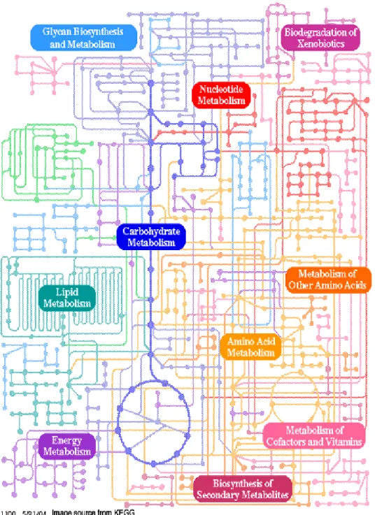
Figure 1.1: Metabolic map as a set of dots and lines. The heavy dots and lines

trace the central energy-releasing pathways known as glycolysis and the citric

acid cycle. (Adapted from KEGG) each intermediate = black dot, each enzyme =

a line. The numbers of dots in the figure have one or two or more lines

(enzymes) associated with them. A dot connected to just a single line must be

either a nutrient/storage form/end product, or an excretory product of

metabolism. Also, since many pathways tend to proceed in only one direction

(that is, they are essentially irreversible under physiological conditions), a dot

connected to just two lines is probably an intermediate in only one pathway and

has only one fate in metabolism. If three lines are connected to a dot, that

intermediate has at least two possible metabolic fates; four lines, three fates; and

so on. ...8

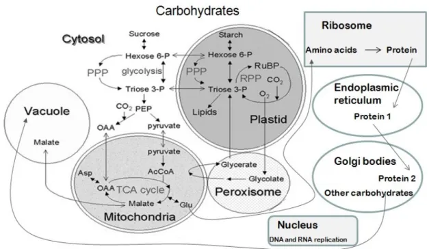
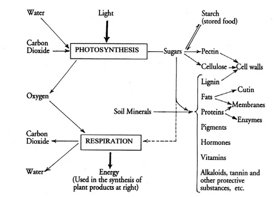
Figure 1.2: An outline of plant metabolism...10

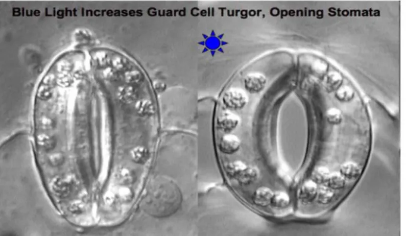
Figure 1.3: Stomatal conductance (Taiz and Zeiger, 1998)...12

Figure 1.4: Material transport through xylem and phloem vessels [Int. ref.2]....14

Figure 1.5: Root structure [Int. ref.1]...16

Figure 1.6: Germination mechanism in lettuce seeds (Int. ref. 5)...19

Figure 1.7: Compartmentation of metabolic processes in a leaf cell. For each

subcellular compartment, some of the major metabolic processes are shown.

Many processes occur exclusively in a single compartment but may obtain their

substrates from, and export their products to, other compartments. Abbreviation:

OAA = oxaloacetic acid, PEP = phosphoenol pyruvate, Glu = glutamine, Asp =

Aspartate, AcCoA = Acetyl CoA, CO2 = Carbon dioxide, O2 = Oxygen, Triose

3-P = Triose 3-phophate, Hexose 6-P = Hexose-6-phophate, PPP = pentose

phosphate pathway, RPP = reductive pentose phosphate pathway. (This image is

inspired from Morgan and Rhodes, 2002)...25

Figure 1.8: General Metabolic model structure for plant metabolic model...36

Figure 2.9: Mathematical way to construct metabolic model (Wiechert and

Takors, 2004)...44

Figure 2.10 : A biochemical system...46

Figure 2.11: Energy balance...47

Figure 2.12: Hypothetical system at steady state...51

Figure 2.13: Mathematical representation of plant metabolic network The

application of constraints reduces the allowable solution space which makes

easier the plant modelling (Adapted from Price et al., 2004)...53

Figure 2.14: Applications and methodologies in the stoichiometric modelling

framework There are two main categories – i) to study the properties of the

whole space of possible flux distributions ii) determination of particular flux

solutions of the allowed space. The scheme is adapted from Llaneras and Pico,

2008; Gombert and Nielsen, 2000...54

Figure 2.15: In silico representation of metabolic network...58

Figure 2.16 : A simplified network ...65

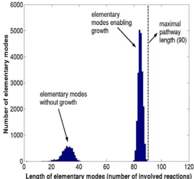
Figure 2.17 : Pathway length distribution of the E. coli modes on glucose.

Maximum pathway length is the maximum no. of reactions involved in

elementary mode (Gagneur and klamt, 2004) ...74

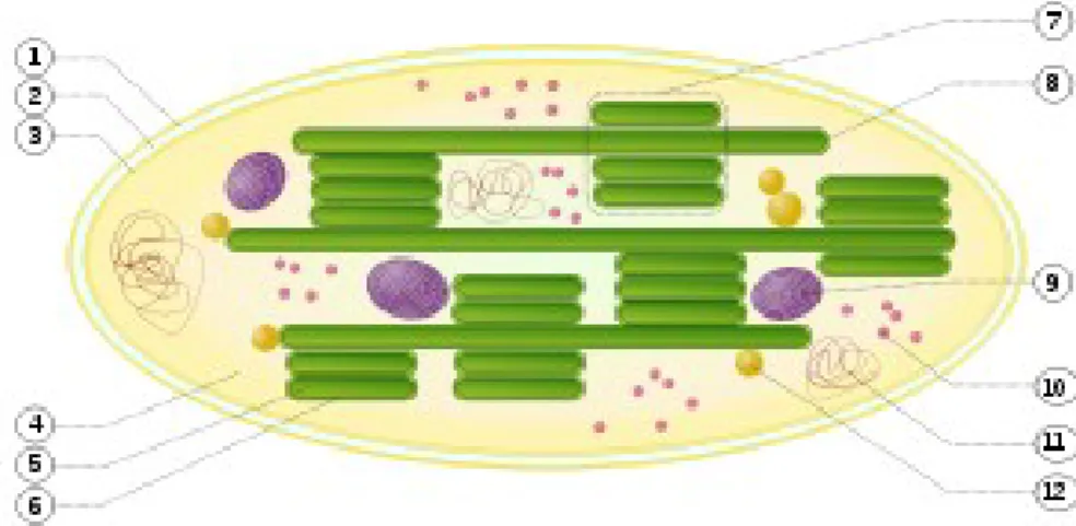
Figure 3.18: Structure of chloroplast 1. outer membrane 2. intermembrane space

3. inner membrane (1 + 2 + 3: envelope) 4. stroma (aqueous fluid) 5. thylakoid

lumen (inside of thylakoid) 6. thylakoid membrane 7. granum (stack of

thylakoids) 8. thylakoid (lamella) 9. starch 10. ribosome 11. plastidial DNA 12.

plastoglobule (lipids)...86

Figure 3.19: Light reactions involving photosystem I and photosystem II

Abbreviations: P- phase – positive phase, N-phase – negative phase, PS I –

photosystem I, PS II –photosystem II, HP+ - proton in P-phase, HN+ - proton in

N-phase, PQ –plastoquinone, PQH2 –plastoquinol, Fd- ferredoxin complex,

PC-plastocyanin, OEC-Mn2+ complex (Adapted from Feyziyev, 2010)...86

Figure 3.20: Z-scheme of photosynthesis Photosynthetic electron flow from

H2O to NADP+. The relative redox potentials show that P680 and P700 are

highly oxidising. Their excited forms (P680* and P700*) of the reaction centre

pigments are highly reducing and located in the upper part of the diagram.

Electrons are transferred from water, through YZ to reduce P680 •+. Further,

P700 •+ is reduced by electrons from PSII, transferred via plastoquinol, through

Cyt b6f complex and plastocyanin (PC). (Picture is adapted from Feyziyev,

2010)...90

Figure 3.21 : Proton movement at Complex II...92

Figure 3.22: ATP synthesis in chloroplasts The CF1-part sticks into stroma,

where dark reactions of photosynthesis (Calvin cycle) take place. The CFO

subunit spans the photosynthetic membrane and forms a proton channel through

the membrane. CF1 is composed of several different protein subunits. The top

portion of the CF1 subunit is composed of three ab-dimers that contain the

catalytic sites for ATP synthesis...98

Figure 3.23: Separation of metabolites into non exchangeables and

exchangeables for light reactions ...98

Figure 3.24: Structure of mitochondrion [Int. ref.3]...104

Figure 3.25: Electron transport pathway via Complex I Proton transport takes

place from N-phase to P-phase (Adapted from Garrett and Grisham, 2000)....106

Figure 3.26: Electron transport pathway via Complex II. (Adapted from Garrett

and Grisham, 2000)...108

Figure 3.27.1 First part of Q-cycle of complex III. The electron transfer pathway

following the oxidation of the first molecule of UQH2 at the Qp site near the

cytosolic face of the membrane (P-phase). (Adapted from Garrett and Grisham,

2000)...110

Figure 3.28: Mechanism for the reduction of oxygen at Complex IV Protons

required for the reduction processes are taken from matrix side or P-phase.. . .116

Figure 3.29: ATP synthesis in mitochondrion Flow of protons through ATP

synathse turns the rotor and ATP released along with water. (Garrett and

Grisham, 2000)...118

Figure 3.30: Separation of metabolites into non exchangeables and

exchangeables for mitochondrial electron transport and oxidative

phosphorylation...120

Figure 3.31: Metabolic reactions involved in mitochondrial electron transport

and oxidative phosphorylation for ATP production...120

Figure 3.32: Electron transport, oxidative phosphorylation and Krebs cycle

reactions...123

Figure 3.33 : System with inputs and outputs...127

Figure 3.34: System with inputs and outputs ...130

Figure 3.35: Mitochondrial electron transport and oxidative phosphorylation

system with inputs and outputs...131

Figure 3.36: Krebs cycle system with inputs and outputs ...133

Figure 3.37: Metabolic flux distribution for light reactions ...137

Figure 3.38: Metabolic flux distribution for Calvin cycle reactions Glucose =

100µ mols-1...139

Figure 3.39: Various possibilities of oxidative phosphorylation in mitochondria

141

Figure 3.40: Metabolic flux distributions for Krebs cycle and Glycolysis...144

Figure 3.41: Metabolites involved in photosynthesis...147

Figure 3.42: Flux distributions for photosynthesis: (a) method 1 (b) method 2

157

Figure 3.43: Flux distribution for respiration: i) method 1: (a) Glucose = -200 µ

mol 1, O2 = -300 µ mol 1 (b) Glucose = -100 µ mol 1, O2 = -100 µ mol

s-1; ii) method 2 (c) Glucose = -200 µ mol s-1, O2 = -300 µ mol s-1(d) Glucose =

-100 µ mol s-1,O2 = -100 µ mol s-1...159

Figure 4.44: Metabolic network model involving central carbon metabolism in

different cell compartments: chloroplast (Calvin cycle), mitochondria (Krebs

cycle), cytosol (Glycolysis), peroxisome, ribosome and vacuole. Violet colour

-repeating reactions, red colour- energetic reactions, yellow colour- light energy

175

Figure 4.45: Leaf metabolic network for protein and lipid production...176

Figure 4.46: Cyclic reactions involved in the leaf metabolic network...178

Figure 4.47: Flux distribution for leaf model ...181

Figure 4.48 : Comparing predicted and experimental biomass...186

Figure 4.49 : Comparing predicted and experimental nitrogen amount in the

biomass...187

List of Tables

Table 1.1: Compartmentation of cell metabolic functions (Based on spinach

leaves (Winter et al., 1994))...24

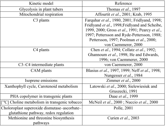
Table 1.2: Kinetic models focusing plant metabolism Part of this table is adapted

from Morgan and Rhodes, 2002...32

Table 1.3: Name and links of familiar metabolic data base...33

Table 2.4 : Applications of elementary flux modes and extreme pathways

analysis in plants and microbial metabolism Adapted from Llaneras and Pico,

2008...61

Table 2.5 : Isotope labelling based MFA, MFA and FBA methods applied in

bacterial and plant metabolism. Adapted from Rios- Estepa and Lange, 2007;

Gombert and Nielsen, 2000; Raman and Chandra, 2009...62

Table 2.6 : Comparison between elementary flux modes and extreme pathways

(Klamt and Stelling, 2002)...69

Table 2.7 Software tools and links for metabolic network analysis...72

Table 3.8: Metabolic steps involved in photosystem II and plastoquinol pool of

chloroplast thylakoids at physiological conditions pHN = 7.5 and pHP = 4...90

Table 3.9: Metabolic steps involved in plastoquinol and plastocyanin of

chloroplast thylakoids. Values with * stands for physiological conditions pHN =

7.5; pHP = 4...93

Table 3.10 : Metabolic steps involved in photosystem I and plastocyanin of

chloroplast thylakoids. Values with * stands for physiological conditions pHN =

7.5; pHP = 4...95

Table 3.11: Metabolic steps involved in ferredoxin NADP reductase of

chloroplast thylakoids. Values with * stands for physiological conditions pHN =

7.5; pHP = 4...96

Table 3.12: Metabolic steps involved in chloroplast ATP synthase Values with *

stands for physiological conditions pHN = 7.5; pHP = 4...98

Table 3.13: Equations for light reactions. Values with * stands for physiological

conditions pHN = 7.5; pHP = 4...100

Table 3.14: Metabolic matrix for light reactions Exchangeables (E): hν700,

hν680, O2, H2O, NADP+, NADPH,HN+, ATP4-, ADP3-, Pi2-, HN+; Non

exchangeables, (NE): HP+, Fdred, Fdox, Pc (Cu+), Pc (Cu2+), PQH2, PQ.

Abbreviations : hν700 and hν680 = photons at 700 nm and 680 nm respectively;

O2 = oxygen; H2O = water; NADPH,HN+ = nicotinamide adenine dinucleotide

phosphate ; NADP+ = reduced nicotinamide adenine dinucleotide phosphate;

ATP4- = adenosine triphosphate; ADP3- = adenosine diphosphate, energy

molecule; Pi2- = inorganic phosphate; HN+ and HP+ = protonated hydrogen at

N and P phases; Fdred = reduced ferredoxin; Fdox = oxidised ferredoxin; Pc

(Cu+) = reduced plastocyanin; Pc (Cu2+)= reduced plastocyanin; PQH2 =

plastoquinol; PQ =plastoquinone...100

Table 3.15: Calvin cycle reactions Free energy values for metabolic reactions

are taken from Bassham and Buchanan, 1982. ...102

Table 3.16: Metabolic matrix for Calvin cycle reactions Exchangeables (E):

H2O; CO2; Glucose; HN+; NADP+; NADPH,HN+; ADP3-; Pi2-; ATP4-; Non

exchangeables, (NE): PGA3-; RuBP4-; Ru5P2-; R5P2-; 1,3-BPGA4-; G3P2-;

DHAP2-; FBP4-; F6P2-; E4P2-; Xu5P2-; G6P2-; S7P2- and SBP4-

Abbreviations : ADP3- = adenosine diphosphate, energy molecule; ATP4- =

adenosine triphosphate; DHAP2- = dihydroxyacetone phosphate; 1, 3-BPGA4-=

1, 3- diphosphate glycerate; CO2 = carbon dioxide ; E4P2- =

erythrose-4-phosphate; FADH2 = reduced flavin adenine dinucleotide; FBP4- = fructose 1,

6-biphosphate; F6P2- = fructose -6-biphosphate; G1P2- = glucose

-1-phosphate; G6P2- = glucose 6--1-phosphate; G3P2- = glyceraldehyde

-3-phosphate ; H2O = water; HN+= protonated hydrogen at N-phase ;

NADPH,HN+ = nicotinamide adenine dinucleotide phosphate ; NADP+ =

reduced nicotinamide adenine dinucleotide phosphate; O2 = oxygen; PGA3- =

3-phosphoglycerate; Pi2- = inorganic phosphate; RuBP4- = ribulose 1,

5-bisphosphate; R5P2- = ribose-5-phosphate; Ru5P2- = ribulose-5-phosphate;

SBP4- = sedoheptulose 1, 7-biphosphate; S7P2- = sedoheptulose-7-biphosphate;

Xu5P2- = xylulose-5-phosphate...103

Table 3.17: Metabolic steps involved in Complex I...106

Table 3.18: Metabolic steps involved in Complex II...108

Table 3.19: Elementary mechanisms of Q cycle of Complex III: Values for near

equilibrium conditions are given for ∆G=0. rL is the ratio of Cyto bL/ Cyto bL-.

rH is the ratio of Cyto bH/ Cyto bH-...116

Table 3.20: Metabolic steps involved in Complex IV...118

Table 3.21: Metabolic steps in mitochondrial ATP synthase...118

Table 3.22: Equations for mitochondrial electron transport and oxidative

phosphorylation...120

Table 3.23: Metabolic matrix for mitochondrial electron transport and oxidative

phosphorylation E = ATP4-, ADP3-, Pi2-, NADH,HN+, NAD+, H2O, O2,

FADH2 , FAD; NE = UQ, UQH2, Cyto(Fe2+), Cyto(Fe3+), HP+,

Abbreviations: O2 = oxygen; H2O = water; NADH,HN+ = nicotinamide

adenine dinucleotide; NAD+ = oxidised nicotinamide adenine dinucleotide;

FAD = flavin adenine dinucleotide ; FADH2 = reduced flavin adenine

hydrogen at N and P phases; CytoFe2+ = reduced iron of heme; CytoFe2+ =

oxidised iron of heme; UQH2 = Ubiquinol; UQ = Ubiquinone...122

Table 3.24: Equations for Krebs cycle (Garrett and Grisham, 2000; Voet D. and

Voet J.G, 2005)...122

Table 3.25: Metabolic matrix for Krebs cycle E = FAD, FADH2, NAD+,

NADH,HN+, H2O, AcetylCoA-, Coenzyme A, HN+, CO2, ADP3-, ATP4- and

Pi2-; NE = Oxaloacetate2-, Citrate3-, cis-Aconitate3-, D-Isocitrate2-, 2–

Ketoglutarate-, Succinyl-CoA-, Succinate2-, Malate2-, Fumarate2- ;

Abbreviations: H2O = water; NADH,HN+ = nicotinamide adenine dinucleotide;

NAD+ = oxidised nicotinamide adenine dinucleotide; FAD = flavin adenine

dinucleotide ; FADH2 = reduced flavin adenine dinucleotide; adenine

dinucleotide; ATP4- = adenosine triphosphate; ADP3- = adenosine diphosphate;

Pi2- = inorganic phosphate; HN+ and HP+ = protonated hydrogen at N and P

phases...124

Table 3.26: Equations for glycolysis (Voet D. and Voet J.G, 2005)...126

Table 3.27: Metabolic matrix for glycolysis E = Coenzyme A ; Glucose ;

NAD+ ; NADH,HN+ ; Pi2- ; ADP3- ; ATP4- ; CO2 ; AcCoA- ; H2O ; NE =

F6P2-; HN+; G6P2-; FBP4-; DHAP2- ; G3P2- ; 2PGA3- ; 3PGA3-; PEP3-; 1-3

BPGA4- ; pyruvate-; Abbreviations: H2O = water; CO2 = carbon dioxide;

NADH,HN+ = nicotinamide adenine dinucleotide; NAD+ = oxidised

nicotinamide adenine dinucleotide; ATP4- = adenosine triphosphate; ADP3- =

adenosine diphosphate; Pi2- = inorganic phosphate; HN+ = protonated hydrogen

at N phase; PEP3- = phosphoenol pyruvate; DHAP2- = dihydroxyacetone

phosphate; 1, 3-BPGA4-= 1, 3- diphosphate glycerate FBP4- = fructose 1,

6-biphosphate; F6P2- = fructose -6-6-biphosphate; G6P2- = glucose 6-phosphate;

G3P2- = glyceraldehyde -3-phosphate ; 2PGA3-= 2-phosphoglycerate ;

3PGA3- = 3-phosphoglycerate; AcCoA- = Acetyl Co A; CoA = Coenzyme A

126

Table 3.28: Obtained elementary flux modes for subsystems of central carbon

metabolism...133

Table 3.29: Metabolic flux distributions for photosynthesis...137

Table 3.30: Metabolites involved in each sub system NE: non exchangeables; E:

exchangeables...145

Table 3.31: Metabolic flux distributions for respiratory system...145

Table 3.32: Metabolic equations for photosynthesis (Method 1)...147

Table 3.33: Metabolic matrix for photosynthesis (Method 1) E = hν700, hν680,

ATP4-, ADP3-, Pi2-, HN+, H2O, CO2, Glucose, O2 ; NE = PGA3-; RuBP4-;

Ru5P2-; R5P2-; 1,3-BPGA4-; G3P2-; DHAP2-; FBP4-; F6P2-; E4P2-; Xu5P2-;

G6P2-; S7P2-; SBP4-; PQ; PQH2; Pc (Cu2+); Pc(Cu+); Fd ox; Fd red; HP+;

NADPH,HN+; NADP+; Abbreviations : hν700 and hν680 = photons at 700 nm

and 680 nm respectively; O2 = oxygen; H2O = water; NADPH,HN+ =

nicotinamide adenine dinucleotide phosphate ; NADP+ = reduced nicotinamide

adenine dinucleotide phosphate; ATP4- = adenosine triphosphate; ADP3- =

adenosine diphosphate, energy molecule; Pi2- = inorganic phosphate; HN+ and

HP+ = protonated hydrogen at N and P phases; Fd ed = reduced ferredoxin; Fd

ox = oxidised ferredoxin; Pc (Cu+) = reduced plastocyanin; Pc (Cu2+)= reduced

plastocyanin; PQH2 = plastoquinol; PQ =plastoquinone; DHAP2- =

dihydroxyacetone phosphate; 1, 3-BPGA4-= 1, 3- diphosphate glycerate; CO2 =

carbon dioxide ; E4P2- = erythrose-4-phosphate; FADH2 = reduced flavin

adenine dinucleotide; FBP4- = fructose 1, 6-biphosphate; F6P2- = fructose

-6-biphosphate; G1P2- = glucose -1-phosphate; G6P2- = glucose 6-phosphate;

G3P2- = glyceraldehyde -3-phosphate ; NADPH,HN+ = nicotinamide adenine

dinucleotide phosphate ; NADP+ = reduced nicotinamide adenine dinucleotide

phosphate; PGA3- = 3-phosphoglycerate; RuBP4- = ribulose 1, 5-bisphosphate;

R5P2- = ribose-5-phosphate; Ru5P2- = ribulose-5-phosphate; SBP4- =

sedoheptulose 1, 7-biphosphate; S7P2- = sedoheptulose-7-biphosphate; Xu5P2-

= xylulose-5-phosphate...148

Table 3.34: Metabolic matrix for photosynthesis (Method 2) E = hν700, hν680,

ATP4-, ADP3-, Pi2-, HN+, H2O, CO2, Glucose, O2; NE = NADPH, HN+;

NADP+...149

Table 3.35: Metabolic equations for photosynthesis (Method 2)...149

Table 3.36: Metabolic equations for respiration (Method 1)...150

Table 3.37 : Metabolic matrix for respiration (Method 1) E = NADH,HN+;

NAD+, HN+; O2; H2O; CO2; ADP3-; Pi2-; ATP4-; Glucose; NE = UQ,

UQH2, Cyto(Fe2+), Cyto(Fe3+), HP+, Fdox, Fdred Oxaloacetate2-, Citrate3-,

cis-Aconitate3-, D-Isocitrate2-, 2-Ketoglutarate-, Succinyl-CoA-, Succinate2-,

Malate2-, Fumarate2-, F6P2-; G6P2-; FBP4-; DHAP2- ; G3P2- ; 2PGA3- ;

3PGA3-; PEP3-; 1-3 BPGA4-; pyruvate- Coenzyme A ; Acetyl CoA- ;

Abbreviations : H2O = water; CO2 = carbon dioxide; NADH,HN+ =

nicotinamide adenine dinucleotide; NAD+ = oxidised nicotinamide adenine

dinucleotide; ATP4- = adenosine triphosphate; ADP3- = adenosine diphosphate;

Pi2- = inorganic phosphate; 2PGA3-= 2-phosphoglycerate ; PEP3- =

phosphoenol pyruvate; DHAP2- = dihydroxyacetone phosphate; 1, 3-BPGA4-=

1, 3- diphosphate glycerate FBP4- = fructose 1, 6-biphosphate; F6P2- = fructose

-6-biphosphate; G6P2- = glucose 6-phosphate; G3P2- = glyceraldehyde

-3-phosphate ; 3 PGA3- = 3-phosphoglycerate; O2 = oxygen; FAD = flavin

adenine dinucleotide ; FADH2 = reduced flavin adenine dinucleotide; HN+ and

HP+ = protonated hydrogen at N and P phases; Cyto(Fe2+) = reduced iron of

heme; Cyto(Fe2+) = oxidised iron of heme; UQH2 = Ubiquinol; UQ =

Table 3.38: Metabolic equations for respiration (Method 2)...152

Table 3.39: Metabolic matrix for respiration (Method 2) E = NADH,HN+;

NAD+, HN+; O2; H2O; CO2; ADP3-; Pi2-; ATP4-; Glucose; NE = FAD,

FADH2, Coenzyme A, Acetyl CoA- ...152

Table 3.40: Metabolic flux distribution for photosynthesis...157

Table 3.41: Metabolic flux distributions for respiration...160

Table 4.42: Available biomass composition (Int. ref. 6)...168

Table 4.43: Available amino acid composition [Int. ref. 6](asn = asparagine; glu

= glutamate)...169

Table 4.44: Available lipid component composition [Int. ref. 6]...170

Table 4.45: Available carbohydrate composition Int. ref. 6...171

Table 4.46: Molar biomass composition...171

Table 4.47 : Stoichiometries involved in different groups of EFMs ‘-‘sign

indicates the energy consumption. The relations for Group [3] are found from

paragraph 4.2.2 ...180

Table 4.48: Model predictions. ‘+ sign’ indicates output components while ‘–

sign’ indicates input components 1) if CO2 accumulation in the biomass is used

as an input 2) if Biomass production is used as an input...184

Table 4.49: Experimental and predicted yields...185

Table 4.50 : Experimental and predicted data comparison...186

Abbreviations

BioCyc Biological database

CESRF Controlled Environment Systems Research Facility (CA)

13_{C MFA Metabolic Flux Analysis using} 13_C

EFM Elementary Flux Modes

EFMA Elementary Flux Mode Analysis EMP Embden Meyerhof Pathway EP Extreme Pathway

EPA Extreme Pathway Analysis ESA European Space Agency ETC Electron Transport Chain FBA Flux Balance Analysis FSA Flux Spectrum Approach Int. ref. Internet reference

KEGG Kyoto Encyclopedia of Genes and Genomes LSS Life Support System

MCA Metabolic Control Analysis

MELiSSA Micro-Ecological Life Support System Alternative MetaCyc Encyclopedia of Metabolic Pathways

MFA Metabolic Flux Analysis

PlantCyc Plant metabolic pathway database TCA Ticarboxylic acid cycle

Atoms, molecules and metabolites

10-formylTHF 10-Formyltetrahydrofolate 1-3BPGA 1,3- bisphospho-D-glycerate

1-3BPGA4- _{Reduced form of 1,3- bisphospho-D-glycerate}

2 Oxo 2-oxoglutarate or 2-ketoglutarate 2-oxobut 2-oxobutanoate

2-oxoiso 2-oxoisovalerate 2PGA 2-phospho-D-glycerate 3PGA - _{3-phospho-D-glycerate}

4-hydroPhe 4-hydroxyphenylpyruvate

5p-ribosyl-1-pp 5-phospho-alpha-d-ribosyl 1-pyrophosphate

ac Acetate

AcCoA- Reduced form of acetyl-CoA

AcCoA Acetyl-CoA

ADP Adenosine diphosphate

ADP3- _{Reduced form of adenosine-diphosphate}

Ala Alanine

AMP Adenosine monophosphate

AMP2- _{Reduced form of adenosine-monophosphate}

Arg Arginine

Asn Asparagine

Asp Aspartate

Asp-semialdehyde Aspartate-semialdehyde ATP Adenosine-triphosphate

ATP3- _{Reduced form of adenosine-triphosphate}

C Carbon

Ca2+ _{Calcium ion (oxidised)}

CH2=THF Methyltetrahydrofolate CH3THF 5-formyl-tetrahydrofolate Cis Aconitate3- _{Reduced form of cis aconitate}

Cit Citrulline

Citrate3- _{Reduced form of citrate}

Cl- _{Chloride ion}

CO2 Carbon dioxide

CoA Coenzyme A

Cys Cystine

DHAP Dihydroxyacetone phosphate

DHAP2- _{Reduced form of dihydroxyacetone phosphate}

DNA Deoxyribonucleic acid E4P D-erythrose-4-phosphate

E4P2- _{Reduced form of D-erythrose-4-phosphate}

F6P D-fructose-6-phosphate

F6P2- _{Reduced form of D-fructose-6-phosphate}

FAD Flavine adenine dinucleotide (oxidised form) FADH2 Flavine adenine dinucleotide (reduced form)

FBP D-fructose-1,6-bisphosphate

FBP4- _{Reduced form of D-fructose-1,6-bisphosphate}

Fe2+ _{Iron ion}

fum Fumarate

Fumarate2- _{Reduced form of fumarate}

G1P D-glucose 1-phosphate

G1P2- _{Reduced D-glucose 1-phosphate}

G3P Glyceraldehyde-3-phosphate

G3P2- _{Reduced glyceraldehyde-3-phosphate}

G6P D-glucose 6-phosphate

G6P 2- _{Reduced D-glucose 6-phosphate}

GDP3- _{Reduced form of guanosine diphosphate}

Gln Glutamine

Glu Glutamate

Glu semi Glutamate-γ-semialdehyde

Gly Glycine

glycerol3P Glycerol 3-phosphate

GTP4- _{Reduced form of guanosine triphosphate}

H+ _{Proton ion}

H2O Water

H2S Hydrogen sulphide

Hexose 6-P Hexose 6-phosphate

His Histidine HN+ Proton in N-phase HNO3 Nitrate HP+ Proton in P-phase icit Isocitrate Iso Isoleucine

Isocitrate2- _{Reduced isocitrate}

K+ _{Potassium ion}

Leu Leucine

Lys Lysine

Mal Co A MalonylcoA

Malate L-malate

Malate2- _{Reduced L-malate}

MethenylTHF 5,10-methenyltetrahydrofolate

Mg2+ _{Magnesium ion}

N Nitrogen

NAD+ _{Nicotinamide adenine dinucleotide}

NADH, H+ _{or NADH Nicotinamide adenine dinucleotide (reduced form)}

NADP+ _{Nicotinamide adenine dinucleotide phosphate}

NADPH, H+ _{or NADPH} Nicotinamide adenine dinucleotide phosphate

(reduced form) NADPH, HN+

Nicotinamide adenine dinucleotide phosphate (reduced form) at N-phase

NADPH, HP+

Nicotinamide adenine dinucleotide phosphate (reduced form) at P-phase

NH3 Ammonia

O Oxygen

O2 Dioxygen (molecular oxygen)

OAA Oxaloacetate

Orn Ornithine

P Phosphorus

PEP Phosphoenol pyruvate

PEP3- _{Reduced phosphoenol pyruvate}

PGA3- _{Reduced 3-phospho-D-glycerate}

Phenyl Ala Phenylalanine Pi Inorganic phosphate

Pi2- _{Reduced inorganic phosphate}

PPi Pyrophosphate

PPP Pentose phosphate pathway

PQ Plastoquinone

PQH2 Plastoquinol

Pr & Pfr Forms of phytochrome

Pro Proline

Pyr Pyruvate

Pyr 5 1-pyrroline-5-carboxylate pyruvate- _{Reduced pyruvate}

R5P Alpha-D-ribose 5-phosphate

R5P2- _{Reduced alpha-D-ribose 5-phosphate}

RBP Ribose 1,5-bisphosphate

RNA Ribonucleic acid

Ru5P D-ribulose 5-phosphate

Ru5P2- _{Reduced D-ribulose 5-phosphate}

RuBisCO Ribulose Bisphosphate Carboxylase-Oxygenase RuBP D-ribulose 1,5-bisphosphate

RuBP4- _{Reduced D-ribulose 1,5-bisphosphate}

S Sulphur

S7P Sedoheptulose 7-phosphate

S7P2- _{Reduced sedoheptulose 7-phosphate}

S-ade-methionine S-Adenosyl-L-methionine S-ad-homocysteine S-Adenosyl-L-homocysteine SBP Seduheptulose-1,7-bisphosphate SBP4- _{Reduced seduheptulose-1,7-bisphosphate} Ser Serine Suc Succinate

Suc CoA Succinyl-CoA Suc homoserine Succinyl homoserine Succinyl-CoA- _{Reduced succinyl-CoA}

THF Tetrahydrofolate

Thr Threonine

Triose 3-P Triose 3-phosphate

Trp Tryptophan

Tyr Tyrosine

UDP Uridine-diphosphate

UDP-glucose Uridine 5'-(trihydrogen diphosphate) alpha-D-gucopyranosyl ester

UMP Uridine-monophosphate

UQ Ubiquinone

UQ.- _{Ubiquinone semi radical}

UQH2 Ubiquinol

UQN.- Ubiquinone semi radical at N-phase

UQP.- Ubiquinone semi radical at P-phase

Val Valine

Xu5P D-xylulose 5-phosphate

Scientific parameters, variables and

notations

* Physiological conditions

A Stoichiometric matrix of ‘m’ metabolites and ‘n’ reactions aa Amino acid

c Velocity of light (2.998 × 108_m/s)

CuA Copper site near mitochondrial P-phase

CuB Copper site near mitochondrial N-phase

Cyt Cytochrome

Cyt b6f Cytochrome b6f Cyt bH Cytochrome bH

Cyt bL Cytochrome bL

Cyt bH- Reduced cytochrome bH

Cyt bL-Reduced cytochrome bL

Cyt c1 Cytochrome c1

Cyt Fe3+ _{Oxidised cytochrome}

Cyt Fe2+ _{Reduced cytochrome}

e Elementary mode e- Electron

E Exchangeables

Em,7 Mid point potential at pH 7 (mV)

Em,4 Mid point potential at pH 4 (mV)

Em,7.5 Mid point potential at pH 7.5 (mV)

Em,6.5 Mid point potential at pH 6.5 (mV)

EN Electrical potential at N-phase (mV)

EP Electrical potential at P-phase (mV)

E Total luminous energy available for one quanta of photon (kJ/mol)

E

∆ Total energy of any system (kJ/mol) F Faraday’s constant (kJ/mol)

Fd Ferredoxin

Fdox Oxidised ferredoxin (Fd(Fe3+₎₎

Fdred Reduced ferredoxin (Fd(Fe2+₎₎

G

∆ Gibbs free energy (kJ/mol)

7 , m

G

∆ Free energy at pH 7 (kJ/mol)

4 , m

G

∆ Free energy at pH 4 (kJ/mol)

5 . 7 , m G

∆ Free energy at pH 7.5 (kJ/mol)

5 . 6 , m G

∆ Free energy at pH 6.5 (kJ/mol)

physio G

∆ Free energy at physiological condition h Planck’s constant (6.626 ×10-34 _J/s)

hν Photon of light

hν680 Photon of light at 680 nm

hν700 Photon of light at 700 nm

J Unknown vector of the reaction rates or fluxes Km Kinetic parameter of Michaelis-Menton constant

n Reactions of a system

n Number of electrons participated in a reaction N Number of amino acids

NE Nonexchangeables or intermediate metabolites N-phase Negative phase

ne Number of protons consumed

∆pH pH gradient between the membranes P680 Reduced pheophytin

P680+ Oxidised pheophytin

P680* Excited photosystem, PS II due to the photon absorption at 680 nm

P700* Excited photosystem, PS I due to the photon absorption at 700 nm

P700 Reduced photosystem, PS I

P700+ Oxidised photosystem, PS I

PC Plastocyanine

PC (Cu2+_{) Oxidised plastocyanin}

PC (Cu+_{) Reduced plastocyanin}

P/2e- Ratio of the production rates of ATP and reduction power of two electrons for photosynthesis (ATP/NADPH, H+₎

pHN pH at N-phase

pHP pH at P-phase

P/O Ratio of ATP production rate and consumption of the reduction power of two electrons for respiration (production of 1 mole of water from ½ mole O2)

P-phase Positive phase II

I,

PS Photosystem I and II

Q Net heat supplied to the system

QA & QB site Sites located at chloroplast and mitochondrial membranes

QN Ubiquinol binding site near N-phase

QP Ubiquinol binding site near P-phase

R Ideal gas constant (8.31451 J/mol K)

R Vector of rates of exchange

E

R Vector of rates of exchange for exchangeables

NE

R Vector of rates of exchange for nonexchangeables rH Ratio of oxidised and reduced forms of cytochrome bH

rL Ratio of oxidised and reduced forms of cytochrome bL

T Temperature (K)

Vmax Kinetic parameter of Michaelis-Menton equation

W Work done by the system

Greek Letters

α Stoichiometric coefficients for lipid formation β Stoichiometric coefficients for lipid formation γ Stoichiometric coefficients for lipid formation δ Stoichiometric coefficients for lipid formation λ Wavelength of light (nm)

−.

~

N

UQ

µ Electrochemical potential of semi ubiquinone radical at N-phase

−.

~

P

UQ

µ Electrochemical potential of semi ubiquinone radical at P-phase ∆Ψ Membrane chemical potential (mV)

Foreword

The project of higher plant growth modelling for life support systems has been developed jointly for two aspects: the global model design with a specific accent on mass and energy transfers, and the simulation of the biomass production at the level of metabolism and plant growth stoichiometry. These studies are presented in the thesis manuscripts of Pauline Hézard, “Higher plant growth modelling for life support systems: global model design and simulation of mass and energy transfers at the plant level” and Swathy Sasidharan L, “Higher plant growth modelling for life support systems: Leaf metabolic model for lettuce involving energy conversion and central carbon metabolism”. These two documents have a common foreword, defining the main aspects and requirements of the project.

Life support systems requirements

Space exploration includes long-term manned missions as well as planetary explorations, which require life support systems (LSS) designed with a high degree of closure and food regeneration capability. Micro-Ecological Life Support System Alternative (MELiSSA) project of European Space Agency (ESA) is designed in this objective providing a planetary base for continuous life support system of a small crew (from 2 to 6), recycling 100% of air, water and producing at least 40% of food.

This system consists of six separated compartments growing micro- and macro-organisms in order to fulfil all the different recycling steps. One of these is used for growing plants: they are in the last steps of recycling, permitting oxygen, water and food regeneration from carbon dioxide, mineralised water and light. The final aim is to be able to control whole recycling loop in order to fulfil human needs. In this objective, efficient and robust models are necessary for each compartment; they are required to control the environment (temperature, pH, light intensity, etc.) to obtain the required behaviour for the organism. Then, the compartment could provide the required amount of output in terms of gas, liquid and solid (food) to the rest of the loop. The system of control is highly constrained by two specificities: multiple levels and multiple time scales. In terms of levels, four different layers can be described (Dussap et al., 2005): level 0 is the closest to the process; it contains the process measurements and basic controllers for maintaining the adequate set point for an environmental parameter. For example, temperature or pH regulations rely on heater-cooler start and stop or acid-base pumps, with a simple proportional-integral-derivative (PID)

controller. Level 1 contains the system model itself, which corresponds to the present work. It states the correct value for each environmental parameter based on the system history, prediction determination and overall loop requirements. Level 2 is not specific for one compartment, but regulates all the set points in an optimisation objective in order to respond to level 3 requirements. Level 3 is the interface with the crew, who can define future events (like crew member arrival or departure) and accurate environmental tuning. This level defines the optimised response of the loop in order to fulfil these requirements. In terms of control dynamics, they are highly different depending on the different states of the matter: gas control has to be effective within few minutes, liquid control is at an hourly step, and food control is in the day scale. Moreover, depending on each compartment, the biological response kinetics to environmental adjustment is different and these various time scales have to be accounted in the models. For the output control, quality and security aspects have to be included: quality in terms of chemical and microbiological content to be provided to the consumers (human crew for the overall system, but also each compartment); and security for the backup systems that should be included at each key point, for each step of the closed loop process. Another important issue is that the life support system functions with uncontrolled inputs, for example, CO2 production rate from the crew cannot be predicted accurately. Additionally, these inputs

may be discontinuous (crew waste production) for a system that is designed for a continuous functioning; this means that all the system is constrained by the mass balance of the overall loop, for all the chemical elements. In a mass- and volume-limited environment in space, the buffer sizes have to be small for each of the consumable (oxygen, water, food, etc.), which means that the life support system must have a short response-time and a highly adaptable behaviour.

Higher plant compartment requirements

Concerning the higher plant compartment, the growth environment is designed as fully controlled, except for the supply of CO2 and waste issued from the human habitat. The input

flow rate corresponds to the flow rate of minerals (CO2, N-NO3 and N-NH4) coming from the

previous compartments in charge of waste degradation. Light intensity and photoperiod, temperature, humidity, pH of the nutrient solution and electro conductivity are adjusted. The higher plants’ growth model should be designed for organising the cultures, and if possible, managing environment in order to control plant behaviour. The main requirements are of three ranges. First, for a closed loop, it is necessary to follow mass balance principle at each

step. Then, the model for higher plant compartment should take into account mass balance: metabolism has to be considered, even if a simplified way with few, global stoichiometric equations. Secondly, this model is only a part of MELiSSA loop control system: it has to be able to communicate information with the models of the other compartments. As it is also a long-term implementation system, it should be built in a structured form in order to be easy to modify, just changing specific functions or adding new parts, if necessary. Finally, the system will be settled in extraterrestrial places: the environmental conditions may not be similar to Earth’s conditions, especially in terms of gravity and radiations. Therefore, the model has to be based upon known mechanisms and validated equations. This mechanistic approach of modelling could be based upon the understanding of rate-limiting processes for plant growth: the different mechanisms that happen in the organism have a maximum rate depending on few parameters. For example, maximum light interception depends on leaf properties (surface, absorption coefficient, etc.) and incident light intensity. These parameters have to be included in the model in order to obtain an accurate value of light energy available for plant growth. If all the maximum rates are calculated (such as water, CO2, nutrient availability), it is possible

to know which rate limits plant growth. Following all these objectives, an extensive bibliographic research was made for finding existing models of plant growth. They can be separated in three categories as described below: global models, models of physical mechanisms and models of biochemical mechanisms.

Existing plant growth models

Global models

Global models can be separated in two main types: process-based models and functional-structural models.

Process-based models consider the environment as the main driving variable for plant growth. The calculation of soil and atmosphere variations depending on climatic conditions and plant interactions permit the calculation of biomass growth and development, in a more or less detailed view. Process-based models take into account some of the growth mechanisms like light interception or water and nutrient absorption. However, plant shape is usually simplified as root and shoot, and/or edible and inedible. These models have the aim of modelling plant growth in an explanatory way linking environment characteristics to plant growth and development; however the developmental steps are included in an empirical way (Bouman et

al., 1996; Boote et al., 1998;Gabrielle et al., 1998; Brisson et al., 2008; Priesack and Gayler, 2009).

Functional-structural plant models are based upon plant architecture. They consider the plant shape (structure) in a detailed way; the internal plant mechanisms are often included in a simplified, sometimes empirical way (Fournier and Andrieu, 1998, 1999; Yan et al., 2004; Allen et al., 2005; Evers et al., 2005; Cournède et al., 2006; Bertheloot et al., 2008).

Of the existing global models of plant growth, all include an original approach of specific mechanisms: process-based models are usually well-structured for all of the mechanisms, and the limiting rates are calculated for predicting water or nutrient stress and eventually pests. Even if they often contain empirical simplifications for some processes, the approach and results are mainly based on extensive experimental knowledge from agriculture results. Also, soil and atmosphere dynamics can be included in an accurate mechanistic way, and the aim of guiding agricultural practices corresponds to the objective of the life support system control. Finally, functional-structural plant models include an accurate approach of morphology (even if the laws of architectural growth are not really mechanistic), and an explanatory or mechanistic approach for some of the mechanisms. Some of them calculate the exact repartition of light and its absorption in the leaves; others take into account a mass-balance approach for biomass repartition in the different organs, etc. That is why, even if none of them can be adapted directly to MELiSSA modelling approach, they can all give interesting ideas for building a new model. Consequently, it is necessary to take into account models of specific mechanisms in order to select suitable ones.

Physical models

The models of plant physical mechanisms for a general plant are studied separately and the influences of specific parameters or conditions are tested in detail. The main mechanisms are light interception, gas exchange, sap conduction and root uptake. Most of them have been built on mechanistic or explanatory laws.

Light interception is generally represented using Beer-Lambert law, at the global or local scale, eventually including the reflection and refraction indices, differentiation between leaves receiving direct or diffuse light, the leaf properties such as leaf angle, height or density (repartition in space), etc. (Govaerts, 1996; Asner and Wessman, 1997; Chelle and Andrieu, 1998; Wang and Leuning, 1998).

Another mechanism is the gas exchange; it happens through the stomata, small dynamic holes in plant cuticles; it depends on stomatal aperture, wind speed in external atmosphere, leaf shape, CO2 concentration difference between atmosphere and leaf. Stomatal aperture is an

important active mechanism based upon osmotic regulations which are controlled by sensing the parameters like light intensity, internal CO2 concentration, atmosphere humidity or water

availability at the root level. Gas exchange depends, also on the atmosphere dynamics around the leaves, leaf shape and canopy architecture. Many different types of models exist, depending if they consider atmosphere dynamics (Boulard et al., 2002), stomatal aperture (Aalto et al., 1999; Dewar, 2002; Kaiser, 2009), CO2 diffusion (Leuning, 1995), water

transpiration (Monteith, 1981) or several of these mechanisms (Tuzet et al., 2003; Xu and Baldocchi, 2003; Zavala, 2004).

The matter exchange between leaf and root happens via sap conduction vessels, which are separated into two different types depending on the sap composition, origin and role: phloem sap contains water and organic solutes produced by photosynthesis in the leaves and provide the organic substrates as building blocks for biomass production in the non-photosynthetic organs: buds, roots, fruits or grains and storage organs. For the movement of water and mineral nutrients from the roots, xylem vessels are made of dead lignified cells allowing a rapid upstream flow. Sap flow rate depends on vessel radius, length, sap viscosity and production (source) and demand (sink) powers, which are expressed as water potential. Only one mechanistic model of phloem exists, based on the pressure difference between production and consumption sites (Christy and Ferrier, 1973; Henton et al., 2002). Usually, only the source and sink powers of the organs and a resistance-to-transfer factor are taken into account in order to model directly biomass repartition in global models (Yan et al., 2004; Allen et al., 2005). For xylem, in many cases, the transport is not considered limiting compared to evaporation mechanism of transpiration, however some models consider this resistance (Tyree, 1997; Da Silva et al., 2011).

Last important mechanism is the root absorption. It depends on root architecture and morphology, nutrient and water availability, active uptake mechanisms, root permeability and pumping power (water potential difference). Several models exist with different parameters and structures (Fiscus and Kramer, 1975; Hopmans and Bristow, 2002; Roose, 2000).

All these mechanisms are extensively studied and most of the models have been established for more than 30 years; however, some parts remain uncertain. The mechanisms which would require some more attention for including accurate and robust mechanistic laws are the

stomatal processes, the sap flow (especially for phloem sap calculation, as it is difficult to measure it experimentally and it is rarely included in the models) and the root absorption. In any case, all the existing laws should be evaluated in order to verify the applicability in the case of controlled but extraterrestrial conditions.

Biochemical models

The biochemical mechanisms exist at two levels: (i) at the cell scale, metabolism, genome transcription-translation regulations, cell multiplication-differentiation, osmotic regulations, etc. (ii) at the plant or organ scale, hormonal signalling, environmental sensing and active transports. However, the latter are poorly described in terms of mathematical formulation, except for metabolism: the role of each hormone, the existence of the sensing systems and the signalling cascade, the cell multiplication and differentiation regulations, especially concerning transcription and translation regulations are not totally understood or known. The large variety of cultivars has given the opportunity to include the genetic variability into some process-based models in order to predict the response of each cultivar to the environment. However, the mechanisms of resistance to a specific pest or environmental stress are not known in detail and the inclusion of cultivar genetic specificities is purely empirical (Bertin et

al., 2010). On the contrary, several modelling tools are available for metabolism; some of

them follow mass-balance principle using stoichiometric equations. They provide the link between matter and energy exchange laws of the physical mechanisms and biomass growth and composition. For other biochemical mechanisms, they could be included in an explanatory way for the known mechanisms, for example, as global laws of development regulation and environmental sensing.

Design of a new model

With the knowledge of existing plant growth models and MELiSSA requirements, a global plant growth model is designed based on the physical and biochemical mechanisms. This corresponds to the structure of a process-based model. However, it should include a detailed description of plant architecture for a functional-structural model. Last requirement is to add a correct mass-balance approach with metabolic stoichiometries. The designed model is schemed in the next page: ‘Part a’ represents the plant mechanisms for the flows of matter and energy, which have to be modelled. ‘Part b’ is the description of the designed model with the details of the flows of information, separated as matter, energy and architecture information.

Figure: Comparison of plant and aimed model structures describing the flows of matter, energy and information.