Fiscal Policy Space and Economic Performance: Some Stylized Facts

HAL Id: halshs-00556996

https://halshs.archives-ouvertes.fr/halshs-00556996

Preprint submitted on 18 Jan 2011

HAL is a multi-disciplinary open access archive for the deposit and dissemination of sci-entific research documents, whether they are pub-lished or not. The documents may come from

L’archive ouverte pluridisciplinaire HAL, est destinée au dépôt et à la diffusion de documents scientifiques de niveau recherche, publiés ou non, émanant des établissements d’enseignement et de

To cite this version:

Céline Carrere, Jaime Melo De. Fiscal Policy Space and Economic Performance: Some Stylized Facts. 2011. �halshs-00556996�

Document de travail de la série Etudes et Documents

E 2007.25

Fiscal Policy Space and Economic Performance: Some Stylized Facts♣♣ ♣♣

Céline Carrère* and Jaime de Melo** November 2007

Summary

This paper complements the cross-country approach by examining the correlates of GDP per capita growth acceleration around “significant” public expenditure episodes by reorganizing the data around turning points, or “events”. Here we define (i) a

growth event as an increase in average per capita growth of at least 2 percentage points (pp) sustained for 5 years, (ii) fiscal event as an increase in the primary fiscal

expenditure annual growth rate of approximately 1 pp sustained for 5 years and not accompanied by an aggravation of the fiscal deficit beyond 2% of GDP. These

definitions of events are applied to database of 140 countries (118 developing countries) over 1972-2005, providing a summary but encompassing description of “what is in the data”.

For this sample, the probability of occurrence of a fiscal event is about 10%, and, for a large range of parameter values for the selection of a “significant” event, the probability of a growth event once a fiscal event had occurred is in the 22%- 28% range. The

probability of occurrence of a fiscal event is higher for the bottom half of the income distribution of countries, but the probability that this fiscal event is followed by a growth event is higher for the third quartile, corresponding to middle income countries (which are largely in Latin America). The probability of a fiscal event not followed by a growth event is significantly higher for the Middle East and Africa region.

The description of the changes in expenditures components during fiscal events shows that, for developing countries, there are notable differences underlying fiscal events followed by growth events: they occur under situations of (i) significant lesser deficit, (ii) fewer resources devoted to non-interest General Public Services and (iii) shift in discretionary expenditures towards Transport & Communication.

After controlling for the growth-inducing effects of positive terms-of-trade shocks and of trade liberalization reform, probit estimates indicate that a growth event is more likely to occur in a developing country when surrounded by a fiscal event. Moreover, the probability of occurrence of a growth event in the years following a fiscal event is greater the lower is the associated fiscal deficit, confirming that success of a growth-oriented fiscal expenditure reform hinges on a stabilized macroeconomic environment (through limited primary fiscal deficit).

♣

We thank Jean-François Brun, Antonio Estache and Peter Heller for comments on an earlier draft.

1.INTRODUCTION

As detailed in World Bank (2007), a renewed focus on fiscal policy and growth has spawned a lively debate over demands for greater “fiscal space” to support growth.1 _{However, there is considerable controversy on what a suitable fiscal}

policy package should look like. Is there a trade-off between the objective of short-term stabilization and long-run growth? Currently, the debate over fiscal policy is cast in terms of “fiscal space” (i.e. availability of a budgetary room to spend more on infrastructure and education for example) and sometimes “macroeconomic space” (possibility to the government to increase expenditure without impairing macroeconomic stability), see Perotti (2007).

As proposed in the recent report to the Development Committee, a growth and development oriented fiscal policy must take into account the composition and efficiency of public expenditures in a framework that includes country’s

conditions (level of indebtedness, and other idiosyncratic characteristics like its access to international financial markets or, in the case of poor countries, to aid). Under this definition, the term “fiscal space” thus refers to a government’s ability to undertake spending to enhance economic growth without impairing its present and future ability to service its debt. 2

So far the exploration of fiscal space and performance has proceeded along three different paths: (i) case studies such as those in the Development Committee report where the performance of 12 countries with different

fiscal/development profiles are contrasted and the complementary high-growth case studies for six countries presented to the Development Committee Meeting of March 2007 (see World Bank, 2007, and Biletska and Rajaram, 2007); (ii) studies of the efficiency of specific public sector expenditures - e.g. the several studies on infrastructure (Calderon and Serven, 2003, 2004, 2005) or on other components of social infrastructure (Estache, Gonzales, and Trujillo, 2007), and (iii) cross-country growth regressions (see the exhaustive summary proposed in Annex 2 of the report for the Development Committee, World Bank, 2007, or

1 _{As defined in the World Bank interim report (2006, p. 1), “the term [fiscal space] initially} applied to the view that fiscal deficit targets limited the ability of government to borrow to finance productive, growth-enhancing infrastructure projects. The term has now gained wider currency, however, and can be seen to refer to constraints to public expenditure which have the potential to raise productivity and yield returns in the future [...]”.

2 _{Depending on individual circumstances, creating fiscal space can occur by increasing}

borrowing and/or raising revenue mobilization, improving the efficiency of public expenditure, and mobilizing more grant aid. The “fiscal space diamonds” used in the interim Report (see World Bank, 2006) is a way to visualize differences across countries. The “diamond” presents the four main options (raise revenue effort; increase borrowing; increase grant aid; improve expenditure efficiency) along four axes departing from coordinates that summarize the country’s current fiscal stance. While a pedagogical and informative way to indicate how fiscal space may be created, this heuristic is not made easily operational.

Perotti, 2007, section 4) in which government expenditures are included among the regressors.

This paper complements the cross-country approach by examining the correlates between significant public spending “chocs” and growth accelerations, reorganizing the data around turning points, or “events”

(calendar time is transformed into “event time”) 3 _{. Does a fiscal “event” precede}

a growth “event”? What are the characteristics of such a fiscal event?

We look for “events” in growth along the lines of Hausman, Pritchett and Rodrik (2005). Lacking information on milestone events in fiscal reforms similar to those available for trade reforms as in Wacziarg and Welch (2003), we define an “event” on the fiscal side using a approach similar to the definition of an event on the growth side, i.e. we define a “fiscal event” based on conditional changes in primary fiscal expenditures.

As explained in the body of the paper, this descriptive analysis faces several challenges. First, as already mentioned, in spite of its focus on growth, the approach certainly captures the stabilization effects of fiscal policy. Actually, our data-constrained definition of fiscal event is based on primary spending that includes also non-discretionary spending. Second, there is arbitrariness in our parameterization of fiscal event, implying a careful sensitivity analysis. Third, the investigation could be viewed as an exploration of the correlates of primary spending choc and growth acceleration and extra care should be exercised when interpreting the results.

Keeping these caveats in mind, the paper unfolds as follows. In section 2, we discuss the relevance of using an event methodology approach and summarize some of our main findings. Section 3 presents the identification conditions of both growth and fiscal events (with details and sensitivity analysis left to the annex A.3). Section 4 studies the characteristics of growth and fiscal events, and the relation between the two. The descriptive analysis computes fiscal event (unconditional) probabilities and probabilities that fiscal events are followed (or not) by growth events. Section 5 investigate the characteristics of fiscal events, in particular the ones followed by a growth event, in terms of geography, underlying changes in expenditure composition, and in the level of associated primary deficit. Then the statistical analysis turns on the growth side, the objective being to see if, based on probit estimates, growth events are more likely to occur in a developing country when surrounded by a fiscal event.

3

The “events methodology” approach has been used in several areas, notably by Bruno and Easterly (1998) for inflation, Wacziarg and Welch (2003) for trade liberalization, and Hausman, Pritchett and Rodrik (2005) for growth and investment performance.

2. THE EVENTS METHODOLOGY

Cross-section growth studies have identified that some public expenditures tend to be “productive” in the sense of being growth-enhancing. In the “standard growth regression” framework, average GDP per capita growth over a decade or more is regressed on a set of “standard” control variables augmented by the inclusion of public expenditure variables.4 _{From the perspective of this study,}

among the more interesting recent developments in these exercises, Kneller et al., 2000, Bose et al., 2003, and Adam and Bevan, 2005, using dynamic panel, have argued persuasively that one should take into account both the sources and the uses of funds simultaneously. Taken together, these recent cross-country studies find that capital expenditure, as well as spending on education, health, transport and communication can be favorable to growth when the government budget constraint is taken into account (see World Bank, 2007 - Annex 2). We retain from these studies that any analysis of fiscal performance should

incorporate the government budget constraint to provide for a meaningful evaluation of the correlates of public expenditures and its relation with growth. Moreover, as pointed out in several studies (e.g. Easterly et al., 1993), growth tends to be highly instable in low-income countries. This makes it more difficult to unveil the relation between growth and its fundamentals. Moreover, as noted by Hausmann, Pritchett and Rodrick (2005) “standard growth theory,

whether of the neoclassical or the endogenous variant, suggests that our best bet for uncovering the relation between growth and its fundamentals is to look for instances where trend growth experiences a clear shift. [...] If instead we lumped together data on growth without paying attention in these turning points, we would be averaging out the most interesting variation in the data.” Here we focus on events that are restricted to GDP growth and primary

spending growth acceleration (an increase in annual GDP per capita growth of at least 2 percentage points and sustained for at least 5 years and on the fiscal side to an increase in primary fiscal expenditure). Rather the fiscal event

captures a change in fiscal stance that likely includes a discretionary component that meets certain qualifications seeking to exclude increases in fiscal

expenditures that could be destabilizing.

As a point of departure, an “events” methodology is purely descriptive. It approaches the robustness problem of the correlates between growth and fiscal expenditures by focusing on turning points in the data, the turning points being defined at discretion. Using threshold values to define events is also a way to

4

Perotti (2007) reviews critically the contributions of the production function and growth regressions emphasizing that the endogeneity of public investment combined with the lack of good instruments casts doubts on the robustness of the results. These criticisms apply to the events methodology as well when interpreting results.

control for some of the fluctuations in the data and to isolate what is under study in a more systematic way than, say, in case studies, since the selection is over a large sample. Actually, we identify fiscal events over the largest possible database including government spending. Moreover, we define conditions on fiscal event in order to take into account the government budget constraint: to qualify as an event, we impose that the increase in fiscal expenditure growth does not occur at the expense of the fiscal deficit.

In sum, while the interpretation of results is subject to caution, this approach provides an easy-to-understand exploration of the correlates between fiscal policy (here fiscal expenditures) and performance (here per capita GDP growth), without imposing a single common linear model for all countries as done in cross-countries regressions. When applied to a large database, as is done in this study, it gives a more encompassing description of “what is in the data” and is thus complementary to the three other approaches mentioned above.

The descriptive analysis computes fiscal event (unconditional) probabilities and probabilities that fiscal events are followed (or not) by growth events. The description of the changes in expenditures during fiscal events shows a shift away from Defense, non-interest general expenditure and Transport & Communication expenditures towards education, health and Housing &

Community expenditures. For the developing country group, there are notable differences in the evolution of expenditures for fiscal events followed by growth events: first fiscal events followed by growth events occur under situations of a significant lesser deficit, and a shift in discretionary expenditures towards

transport & communication is only observed for fiscal events followed by growth events. After controlling for the growth-inducing effects of positive terms-of-trade shocks and of terms-of-trade liberalization reform, the statistical analysis in which the probability of a growth event is conditioned on the occurrence of a fiscal event in surrounding years confirms that growth events are, on average, more likely when a fiscal event has occurred. Moreover, the probability of occurrence of a growth event in the five years following a fiscal event is greater the lower is the associated fiscal deficit, confirming that success of a growth-oriented fiscal- expenditure package likely hinges on a stabilized macroeconomic environment (through limited fiscal deficit).

3.DEFINING EVENTS

We are interested in the relation between a “significant” change in fiscal

spending and a “significant” change in GDP growth - what Hausmann, Pritchett and Rodrick (henceforth HPR, 2005), call “growth acceleration”. Per capita GDP growth and primary fiscal expenditures (in GDP %) growth are then our two indicator values. Call these growth indicators, z . Average annual changes,

, t n

z , are computed for each year over successive windows of length n. Here, because of the limited sample size for the fiscal data (1972 to 2005) we choose a succession of windows of n= years. So we compute 5 ∆z_{t n,} :

, , ,

t n t t n t t n

z z ₊ z ₋

∆ = −

If the change ∆z_{t n,} in the average indicator value satisfies certain conditions (see below), we will say that an “event” has taken place for z in t. The annexes A.1 and A.1 describes in detail the sample and annex A.3 reports how we selected the parameter values defining an event and how sensitive our sample of events is to changes in the conditioning values. Here we summarize the conditions for our ‘benchmark’ set of parameters starting with GDP per capita growth, and then turning to primary fiscal expenditures. In this benchmark case, the sample produces 58 growth events and 95 growth events. Sensitivity of the number of events to the choice of parameter values is reported in the annex A.3, table A.4. Growth events. A growth event will have taken place in t if the following conditions are met:

(i) an increase in the average per-capita growth of 2 ppa or more (percentage points per annum, ppa),

(ii) growth acceleration sustained for at least 5 years [t;t+4],

(iii) an average annual growth rate at least 3.5 ppa during the acceleration period [t;t+4],

(iv) a post-acceleration output exceeding the pre-episode peak level of GDP.

With this selection process, several events could follow one another over

consecutive years capturing in fact the same event. To select the more “relevant” year, we fit a spline regression and choose the year for which the change in indicator value is statistically the most significant. Finally, we impose the

restriction that two events must be separated by at least five years. This method is used for both growth and fiscal events.

Here, we strictly follow HPR in their definition of growth acceleration. However, since there is considerable variation in growth performance associated with terms-of-trade changes, especially for low-income countries (see Easterly et al. 1993), one might also wish to refine the definition of a growth event to purge

from the series the growth accelerations that would be due to changes in the terms-of-trade.5 _{This is done in the statistical analysis of section 5 where we}

control for the impact of changes in the terms-of-trade.

Fiscal Events. The core of this study is the definition of a fiscal event. Ideally, we would like to carry out the equivalent of what Wacziarg and Welch (WW, 2003) have done for trade liberalization episodes, that is use a combination of criteria that qualify a fiscal reform to center an event which could then be checked against detailed reports identifying significant changes in the fiscal regime. In a second step a “before and after” analysis would be carried out around the fiscal event for selected outcome indicators (e.g. growth and other indicators like investment in the case of WW).

Unfortunately, carrying out a similar exercise for changes in fiscal policy is much more difficult. First, as mentioned above, is the issue of trying to disentangle the stabilization objective from the growth objective which is not addressed here. Second, there is much more fungibility in fiscal policy than in trade policy, so it is more difficult to identify the fiscal space levers, and it is much more difficult to identify the expected effects of changes in these levers. Here, we restrict fiscal reform to a change in total primary fiscal expenditures and, in a second step, we study the underlying evolution of many components of potential interest (e.g. education, health or transport and communication) Faced with these limitations and with limited data availability, we rely on changes in consolidated central government total fiscal expenditures, TFE (taken from the GFS, see details in annex A.1) as “event” changes in government expenditures. Since we are looking for autonomous fiscal expenditures, events are defined on expenditures purged of non-discretionary components such as wages and interest payments, IP .6 _{Lacking information on the wage component}

for each functional expenditure category, we consider as discretionary TFE purged of interest payments. So, we define discretionary fiscal expenditure, DFE, as DFE=TFE−IP which is equivalent to focusing on primary spending. We also compute the primary fiscal deficit, def, as the difference between the total revenues and grants and the discretionary fiscal expenditure, DFE (so a deficit is negative).

As discussed below, for the developing countries in the sample used here, average DFE is 24% of GDP and average central government primary fiscal

5 _{While HPR also face this problem, because they use an 8-year (rather than a 5-year) window,} they are less likely to be capturing terms-of-trade fluctuations in their growth events.

6 _{Heller (2006) considers wages and interest payments as the 2 non-discretionary expenditures} in developing countries. In our fiscal data set which is decomposed by “function”‘ rather than “economic” use we do not have a wage component for each function so we cannot include wages as non-discretionary. See the annex A.1 for the definitions of these components.

deficit, def, is -2% of GDP. An increase in DFE will be declaring as fiscal event in t when the following conditions are met over the following five year window:

(i) an increase in DFE average growth of 1 ppa (percentage point per annum),

(ii) If in deficit (i.e def< -2% of GDP), deficit does not increase,

(iii) If in surplus (or in def > - 2% of GDP), the increase in DFE does not lead to a deficit exceeding 2% of GDP

To illustrate, suppose that, under our definition of window (i.e. regressions over 5 year periods), there was no increase in DFE over the previous period, and that DFE was equal to the sample average of 24%. Then condition (i) above will be satisfied for a country if DFE increased by at least 4 percentage points during the 5-year period, i.e. it increased to 28% of GDP. The 5-year (rather than a longer period) window was dictated by the length of the time-series and our desire to have enough fiscal and growth events for statistical analysis. Sensitivity of events to the above conditions is discussed in the annex A.3.

This is a first cut at defining a “fiscal event” and this definition could be

improved upon in several ways. First, the “event” should not be interpreted as entirely discretionary (or unanticipated). The large set of expenditures included in DFE implies that the fiscal event captures non-discretionary elements in the definition and more restrictive definitions of discretionary fiscal expenditures could certainly be built around one of the functional components of fiscal expenditures, although any greater volatility in narrower series may be difficult to interpret.7 _{Thus, the most plausible interpretation of the constructed “events”}

is as significant changes in fiscal policy and refrain from attributing any government objective to the event.

Second, in view of the links we are seeking to establish between fiscal spending events and growth events, one might consider whether the selection of the fiscal event (in particular through conditions (ii) and (iii)) is biased towards selecting as fiscal events those that are followed by growth. Actually, due to the

automatic response of government spending and taxes to output growth, a period of growth acceleration after the fiscal event will lead, other things equal, to a lower deficit. Hence, by construction, we are more likely to select as fiscal events those that are followed by growth since a condition is imposed on the evolution of the fiscal deficit (conditions (ii) and (iii)). This is certainly the case for OECD countries such as Finland, Sweden or Norway that appear in our

7

As discussed by Perotti (2007), it is very difficult even in developed countries like the US where quarterly data and external information on GDP elasticities of revenues and transfers are both available to apply time-series methodologies to detect a fiscal discretionary policy shock (i.e. an unanticipated shock) in the data. Data requirements are too demanding to apply these

event results (see figure 1 below) and that are known for their strong tax revenue elasticities to production (elasticities estimated to be greater than unity). However, as noted by Perotti (2007), among the papers that have studied the cyclical behavior of fiscal policy in developing countries (see e.g. Kaminsky et al., 2004, and Gavin and Perotti, 1997), it seems widely accepted that fiscal policy in these countries is typically pro-cyclical, i.e. the budget deficit is positively correlated with economic growth. 8 _{Hence, according to this}

pro-cyclical effect, if a growth event occurs in the year following a fiscal event, this should increase the deficit, and hence weaken the probability of observing fiscal events followed by a growth event (recall that an increase in discretionary fiscal expenditure associated with an increase in the fiscal deficit does not qualify as a fiscal event). One might even suspect our definition of fiscal event to

underestimate, for the developing countries, the correlation with subsequent growth.

Third, even though the GFS makes an effort at classifying extra-budget items consistently, as already mentioned, data is limited to the Consolidated Central Government while a more suitable aggregate would be based on data for the Consolidated General Government.9 _{Given the quality of the data, we have}

refrained from trying to tune the coarse constraint on deficit improvement imposed here. A natural extension would be to replace conditions (ii) and (iii) by a formal test on sustainability.10 _{Finally, we would not want to exclude}

countries that sought fiscal space through highly confessional borrowing even if this led to an increase in their deficit (since, despite high grant percentage as a share of the loan, such loans are not treated as grants).11 _{This suggests that one}

might wish to take an estimate of the grant component of such loans and include that portion in government revenue thereby relaxing the budgetary constraint. However, there is no data on the grant component of these loans. As an alternative, we redefined our fiscal event with a fourth condition allowing

8 _{Several explanations have been advanced to explain the procyclicality of fiscal policy in} developing countries. Among others, Gavin and Perotti (1997) have argued that developing countries face credit constraints that prevent them from borrowing with slow growth. Tornell and Lane (1999) show that competition for a common pool of funds among different units (ministries, provinces) leads to the so-called “voracity effect” whereby expenditure could actually exceed a given windfall. Alesina and Tabellini (2005) show that procyclicality is an optimal behavior in the presence voters with imperfect information and corrupt politicians. 9 _{86% of the observations rely on data consolidated at the central government sector level and} the remainder 14% at the budget central government level. See annex A.1.3 for further discussion.

10 _{Since the sensitivity analysis to the selection of parameter values reported in annex A.3 gives a} relatively small change in the number of fiscal events over a broad range of parameter values, we refrained from experimenting with a formula that would link the value of the deficit level to the level of indebtedness, or from more formal tests of sustainability such as those used by Chalk and Henning (2001). Moreover these tests have only be done for OECD countries and given the lack of availability in indebtedness data, these improvements in the fiscal event definition seem hardly worth attempting in our sample.

11

Low-income countries to increase their fiscal deficit during the fiscal spending growth period up to 4% of GDP (considering that for low income countries, external borrowing is likely to be on highly concessional terms). Results are reported in next section.

Fourth, with better indicators of performance of government expenditures than GDP per capita growth, this “event-type” analysis could be extended directly to the indicators of fiscal expenditure that concern the debate on fiscal space, e.g. health and/or education expenditures and expenditures on transport &

communication (capturing then, for instance, event in budget reallocation between government functions for a given amount of total outlays).12

4. Patterns of Fiscal and Growth Events

Keeping in mind the shortcomings of this methodology, we take an exhaustive approach by constructing fiscal events for as many countries as possible. Since we are interested in the various components of fiscal expenditures, the best database is the IMF Government Financial Statistics (GFS). GFS statistics are available for a large number of countries since 1972 and up to 2005.13 _Following

most previous studies on fiscal expenditures we use data on fiscal expenditures by function (instead of expenditures by economic classification---i.e. by current vs. capital expenditures). As described in annex A.1, after reconciling the fiscal data, our sample includes 140 countries, of which 118 are developing (i.e. non High Income OECD countries).

Data are described in table 1 which gives decadal averages for the fiscal variables used in the study. A comparison of actual vs. potential observations indicates a large number of missing observations, even for OECD countries, especially over the period 1991-2000 where the coverage is the weakest. For developing

countries, coverage gets better through time with data for half of the potential observations during the nineties. One of the reasons for the small sample (relative to the potential sample) is that we require that data be available for all the components of fiscal expenditures by function, else the year observation is entered as missing and hence excluded from the sample. This lack of data raises the question of biases for the subsequent analysis. In view of the relatively evenly spread out pattern of missing observations across the sample, and in the absence of any other information, we proceed as if there were no selection effects operating via missing data.

12 _{However, as already mention, given the low quality of fiscal data, volatility in narrower series} may be more difficult to interpret.

13 _{There was a major change in the GFS in 1989 causing concern about the comparability of data} before and after that date (see details on the data reconciliation in annex A.1.2). Using box-plots, we explored the possibility of lack of comparability for the series of interest. Fortunately, as discussed in the annex A.1.2 (see figure A1), this is not the case.

Average deficit figures are comparable across the two groups of countries. Regarding our variable of interest—primary fiscal expenditure—the figures are about a third higher for OECD industrial countries partly reflecting a larger revenue base. As defined here, there is no trend in primary expenditures for the two groups of countries over the three decades. As to the components of

expenditures, developing countries spend proportionately more on general public services, on defense and on education, while OECD countries spend more on health.

Table 1: Central fiscal expenditures: average values

1972-1980 1981-1990 1991-2000

High Income OECD countries (22)

Observations (potential number in parenthesis) 159 (198) 179 (220) 129 (220)

Overall deficit in GDP % -.90 -2.47 -1.94

Total public exp. in GDP % 29.21 35.48 33.77

Discretionary public exp. in GDP % a/ 27.79 32.05 30.49

Expenditures by function (in % of total public exp.) 100 100 100

General public services of which 17.7 22.2 22.9

interest payment (4.9) (9.7) (9.7)

Defense 8.4 6.8 5.6

Transport and Communication 6.8 5.0 3.7

Housing and community amenities 2.3 2.1 2.0

Health 9.7 10.0 10.8

Recreation, culture, and religion 0.9 0.9 1.0

Education 9.4 7.9 7.2

Others (residual) 40.0 35.5 37.1

Developing countries (118)

Observations (potential number in parenthesis) 360 (1062) 433 (1180) 644 (1180)

Overall deficit in GDP % -2.57 -2.38 -1.93

Total public exp. in GDP 23.58 26.45 25.44

Discretionary public exp. in GDP % a/ 22.40 23.86 22.66

Expenditures by function (in % of total public exp.) 100 100 100

General public services of which 28.3 27.9 28.0

interest payment (5.0) (9.8) (10.9)

Defense 12.3 11.3 10.4

Transport and Communication 9.6 8.0 5.6

Housing and community amenities 2.9 3.1 3.2

Health 6.4 6.5 6.9

Recreation, culture, and religion 1.5 1.2 1.4

Education 14.7 13.7 13.4

Others (residual) 19.3 18.4 20.1

Notes: See annex A.1.3, table A.3 for country classification in the sample.

a/ defined as total public expenditures less interest payments. See annexes A.1 and A.2 for details on definition and construction of variables.

For the growth database, we use the Penn World Table PWT 6.2 as our baseline data source.14 _{Hence, the “growth” database covers 187 countries over the same}

period as the fiscal data base, i.e. 1972-2004. Taking into account missing data, the sample includes 5380 observations hence 87% of the potential number of observations (=6171=187 countries*33 years).

Turn now to the construction of growth and fiscal events as defined in section 3 and in the annex A.3. Due to the availability of GFS data since 1972, we have a shorter time-series than HPR. This implies that we cannot use periods as long as HPR who used GDP data going back to 1950, leading them to choose 8-year periods, i.e. n= and giving them events over the period 1958-1992 (GDP data 7 available until 1999). As mentioned above, due to the limitations imposed by the availability of fiscal data, we choose 5-year periods for both fiscal and growth events, i.e. n= . This means that the exercise covers the period 1977-2000.4 15

Because there is missing data, we have also imposed that data be available for 4 out of the 5 years entering each “window”. If this condition is not satisfied, a missing value is entered for that “window”.

Having computed the fiscal and growth events on their respective databases, we merge the two into a final dataset (see annex A.2 for details). The resulting database includes 107 countries (84 developing countries, i.e. all non- High Income OECD countries), over 1977-2000. This leads to 1452 observations hence 57% of the potential number (=2568=107 countries*24 years).

As indicated in the annex A.3--where we carry out sensitivity analysis with respect to the selection of parameter values in defining events--for this sample and for the parameter values selected here, we get 58 growth events and 95 fiscal events (see table A.4 for the number of events obtained when we change parameter values over the sample). This is our benchmark data set over which exploration takes place. As discussed in table A.4, the number of events is relatively insensitive to a range of plausible parameter values. Nor are changes in the pattern of events surprising when we change parameter values.

Figure 1 plots a subset of events in this benchmark case: 25 fiscal events are simultaneous or followed by a growth event, 23 fiscal events are preceded by a growth event. The residual (47) events that are neither followed nor preceded by a growth event are not shown in the figure (also see the details in table A.4).

14 _{Using WDI database is an alternative. However, as shown by HPR, this does not affect the} results.

15 _{When we define n=8 instead of 5, the period under study shrinks to 1980-1997 and we get 52} fiscal events and 18 growth events.

Figure 1. Growth events vs. fiscal events

Notes:

- 19 points strictly above the red line (growth event strictly preceded by fiscal event); - 23 points strictly below the red line (growth event strictly followed by fiscal event); - 6 points on the red line (growth event simultaneous to fiscal event, of which 4 in Latin

America).

95-48=47 fiscal events with no associated growth events not shown in the figure.

ARG: Argentina; BTN: Bhutan; CHL: Chile; CMR: Cameroon; CRI: Costa Rica; DOM:

Dominican Republic; FIN: Finland; GBR: United Kingdom; HUN: Hungary; IRL: Ireland; ISL: Iceland; ISR: Israel; KOR: Korea, Rep.; LSO: Lesotho; MEX: Mexico; MLT: Malta; MYS: Malaysia; NOR: Norway; PAN: Panama; PNG: Papua New Guinea; SGP: Singapore; SWE: Sweden; URY: Uruguay.

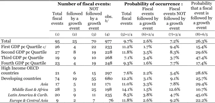
Table 2 reports unconditional probabilities of these fiscal events.16 _{For the}

whole sample and given our construction of a fiscal event, the probability of occurrence of a fiscal event is 9.7% and the probability of a growth event once a fiscal event has occurred is 26.3%. Table 2 also reports probabilities across countries ranked according to their income per capita and by region). Column 5 shows that, although the probability of occurrence of a fiscal event is fairly evenly spread across the income quartiles, the probability is higher for the lower quartiles (first and second). It is difficult to interpret this pattern since, as

explained above, this definition of a fiscal event does not distinguish between fiscal policy shocks and systematic fiscal policy. If one can assume that fiscal policy shocks are not more prevalent among low and middle income countries, then the pattern would seem to indicate that fiscal policy is more volatile among low-income countries. The probability that a fiscal event is followed by a growth event is much higher for the third quartile (i.e. for middle-income countries which are largely in Latin America). Note however, that the patterns suggest that fiscal policy may be pro-cyclical (but not destabilizing given our definition of fiscal event) in Latin America since, out of the 9 fiscal events associated with growth in Latin America, 4 are simultaneous (see figure 1), which seems to confirm earlier results (see e.g. Gavin and Perotti, 1997, Kaminsky et al. 2004 and Perotti, 2007).

The bottom part of table 2 shows that developing (i.e. non High Income OECD) countries almost have twice as high a probability of a fiscal event occurrence than industrial countries. At the same time, developing countries are less likely to have a growth event following a fiscal event. Within the developing country group, as already noted, Latin America stands out with both the lowest

probability of occurrence of a fiscal event, and the highest probability that the event is followed by a growth event.

It is instructive to compare, side by side, probabilities of a fiscal event with the probability of a fiscal event followed by a growth event. This is done in figure 2. Consider first figure 2a. It is clear that low-income countries have both a higher probability of having a fiscal event, but a lower probability of having a fiscal event followed by a growth event. Looking at it by region in figure 2b, one sees

16 _{These probabilities are computed by dividing the numbers of events by the number of} country-year observations in which an event could have occurred. The latter is calculated by summing all the observations in the sample and eliminating: (i) a 4-year window after the occurrence of each event since our qualifying conditions take this period as belonging to the same episode; (ii) the potential competing dates before the event that have been eliminated by the spline regression. This rule gives 977 possible occasions in which a fiscal event could have occurred, i.e. the probability of a fiscal event is: 95/977=9.7% (see table 2 col. 5) for a typical country over the full-sample period 1977-2000. Likewise, a typical country would have about 2.6% (col. 6) probability of experimenting a fiscal event followed by a growth acceleration at some point over 1977-2000. This means that the probability of growth acceleration when a fiscal event has occurred is around 26.3% (table 2, col. 8).

that this pattern is largely reflecting the distribution of fiscal and growth events in the Middle East and Sub-Saharan Africa. Suppose then that the success of a fiscal event can indeed be measured by whether or not it is followed by a growth event. One is then tempted to add that these patterns could reflect the quality of underlying institutions. Indeed, according to many indicators, Sub-Saharan Africa and the Middle East have bad scores on several indicators of institutional quality.

Note that when we use the alternative definition of fiscal event allowing Low-income countries to increase their average fiscal deficit during the fiscal

spending growth period up to 4% of GDP, 3 additional fiscal events followed by a growth event are identified: Mali, Mauritius and Burkina Faso. Then, under this scenario, the probability that a fiscal event is followed by a growth event in Middle East and Africa increases from 11% to 21%.

Table 2. Fiscal event probabilities a/

Number of fiscal events: Probability of occurrence : Total fiscal events followed by a growth event NOT followed by a growth event obs. b/ Total fiscal events Fiscal events followed by a growth event Fiscal events NOT followed by a growth event Probability that a fiscal event is followed by a growth event (1) (2) (3) (4) (5)=1/4 (6)=2/4 (7)=3/4 (8)=6/5 Total 95 25 70 977 9.7% 2.6% 7.2% 26.3% First GDP pc Quartile c/ 26 4 22 233 11.2% 1.7% 9.4% 15.4% Second GDP pc Quartile 27 8 19 228 11.8% 3.5% 8.3% 29.6% Third GDP pc Quartile 19 9 10 268 7.1% 3.4% 3.7% 47.4% Fourth GDP pc Quartile 23 4 19 248 9.3% 1.6% 7.7% 17.4%

High Income OECD

countries 21 6 15 297 7.6% 2.2% 5.4% 28.6%

Developing countries 74 19 55 680 12.2% 3.1% 9.1% 25.7%

Asia 17 5 12 171 11.0% 3.3% 7.8% 29.4%

Middle East & Africa 28 3 25 198 14.1% 1.5% 12.6% 10.7%

Latin America & Carib. 20 9 11 235 8.5% 3.8% 4.7% 45.0%

Europe & Central Asia 9 2 7 76 11.8% 2.6% 9.2% 22.2% Notes: See annex A.1.3, table A.3 for country classification in the sample.

a/ Computations based on benchmark set of parameters from table A.4, row 1 (58 growth events and 95 fiscal events).

b/ Obs. in which a fiscal event could have occurred.

c/ “First GDP pc Quartile” corresponds to “low income” and some “lower middle income” countries. “Second GDP pc Quartile”: “lower middle income" and some "upper middle income” countries. “Third GDG pc Quartile”: “high income” countries.

“Fourth GDP pc Quartile”: “upper middle income” countries.

Figure 2. Fiscal and Growth event probabilities by income quartiles and regions a. by GDP per capita Quartiles (“Fourth” is the highest)

%: probability of growth acceleration when a fiscal event has occurred

b. by regions

%: probability of growth acceleration when a fiscal event has occurred Source: computation from Table 2, cols 5 and 8.

5. Understanding Fiscal Events:

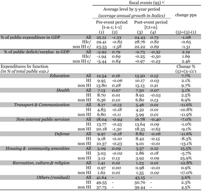
The Anatomy of fiscal Events. The benchmark set of parameters selected 95 fiscal events. Table 3 describes the changes in the composition of fiscal

expenditures around these events. The table shows average values and changes for the 5-year period preceding the event and the 5-year following the event. Table 4 gives the same information, but this time the comparison is between events that preceded a growth event and events that did not precede a growth event, focusing on “Low and Middle Income” countries.

Start with the anatomy of fiscal events in table 3. Not surprisingly, the

restriction that fiscal events in deficit situations should be accompanied by a reduction in the fiscal deficit is reflected in the evolution of the fiscal deficit (reduction) between the periods preceding and following the event date. The patterns are the same for both groups of countries (i.e. High and non-High income countries), average changes (see last column) being larger for the Low and Middle Income country group. Likewise, individual changes in expenditures by functional group are larger for Low and Middle Income than for High Income countries. However, the pattern of changes for the big expenditure categories is the same for both groups of countries.

One can check if there are noticeable differences in the changes in expenditures across the two groups. Taking the whole sample and ignoring the residual category, fiscal events involve a shift towards Education, Health and Housing & Community expenditures at the expense of Defense, non-interest General Public Services, and Transport & Communication expenditures. For the Low and

Middle Income country group, the three big expenditure items are (percentage of discretionary expenditures in parenthesis): non-interest Public Services (20.2%), Education (13.8%) and Defense (10.4%). Compared with the High Income events, the Low and Middle Income country events indicate a much bigger cut in non-interest public services and in defense expenditures, the latter probably capturing countries entering a post-conflict situation.

Table 3: Characteristics of fiscal events

fiscal events (95) a/

Average level by 5-year period (average annual growth in Italics)

Pre-event period Post-event period

change ppa

[t-n-1; t-1] [t;t+n]

(1) (2) (3) (4) (5)=(3)-(1) % of public expenditure in GDP All 25.51 -1.33 24.43 0.73 -1.08

HIc/ 29.41 -0.85 28.76 0.82 -0.65 non HI c/ 23.53 -1.58 22.22 0.69 -1.31 % of public deficit/surplus in GDP All -2.92 0.79 -0.73 -0.32 2.19 HIc/ -1.94 0.69 -0.25 -0.50 1.69 non HI c/ -3.44 0.84 -0.97 -0.23 2.46

Expenditures by function Change %

(in % of total public exp.) (5)=(3-1)/1

Education All 12.54 0.16 13.50 0.15 7.7% HI 9.95 -0.06 10.17 0.03 2.1% non HI 13.80 0.28 15.13 0.21 9.7% Health All 7.13 0.07 7.50 0.07 5.1% HI 8.70 0.01 8.92 -0.03 2.5% non HI 6.36 0.10 6.80 0.13 6.9% Transport & Communication All 6.17 -0.13 5.46 0.01 -11.6%

HI 4.83 -0.18 4.32 0.01 -10.8% non HI 6.80 -0.11 5.99 0.01 -11.9% Non-interest public services All 18.04 -0.94 16.78 -0.40 -7.0% HI 13.77 -0.25 13.64 0.09 -1.0% non HI 20.18 -1.30 18.35 -0.65 -9.1% Defense All 9.97 -0.18 8.82 -0.06 -11.6%

HI 9.18 -0.10 8.42 -0.15 -8.3% non HI 10.37 -0.23 9.01 -0.01 -13.1% Housing & community amenities All 3.09 0.09 3.57 0.12 15.5%

HI 3.03 -0.02 2.86 0.18 -5.7%

non HI 3.12 0.15 3.92 0.09 25.9% Recreation, culture,& religion All 1.41 0.01 1.23 0.01 -12.8%

HI 0.97 0.00 0.98 -0.01 0.9%

non HI 1.62 0.01 1.35 0.02 -17.0% Others (residual) All 41.64 - 43.15 - 3.6%

HI 49.55 - 50.70 - 2.3%

non HI 37.75 - 39.44 - 4.5%

Notes: See annex A.1.3, table A.3 for country classification in the sample.

Col. 1: average over 5-year period preceding fiscal event; Col. 3: average over 5-year period after fiscal event a/ _{Based on the benchmark set of parameters (table A.4, row 1).}

b/ _{Average annual growth rate over the period in parenthesis}

c/ _{HI stands for “High-Income” countries as defined by World Bank (July 2007);} “HI” sample = 32 fiscal events, “non HI” sample = 63 events.

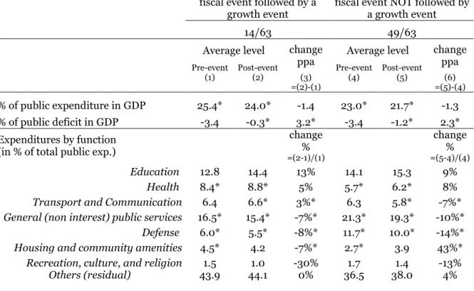
Focusing on the Low and Middle Income country group, table 4 compares the evolution of functional expenditures for fiscal events followed by a growth event compared with those not followed by growth events. In particular, we look at the underlying changes of discretionary public expenditures by function.

Table 4: Characteristics of Fiscal Events in Developing countries According to Their Timing with Growth Events a/

fiscal event followed by a growth event

fiscal event NOT followed by a growth event

14/63 49/63

Average level Average level

Pre-event Post-event change ppa Pre-event Post-event change ppa (1) (2) (3) =(2)-(1) (4) (5) (6) =(5)-(4) % of public expenditure in GDP 25.4* 24.0* -1.4 23.0* 21.7* -1.3 % of public deficit in GDP -3.4 -0.3* 3.2* -3.4 -1.2* 2.3* Expenditures by function

(in % of total public exp.)

change % =(2-1)/(1) change % =(5-4)/(4) Education 12.8 14.4 13% 14.1 15.3 9% Health 8.4* 8.8* 5% 5.7* 6.2* 8% Transport and Communication 6.4 6.6* 3%* 6.3 5.8* -7%* General (non interest) public services 16.5* 15.4* -7%* 21.3* 19.3* -10%*

Defense 6.0* 5.5* -8%* 11.7* 10.0* -14%* Housing and community amenities 4.5* 4.2 -7%* 2.7* 3.9 43%* Recreation, culture, and religion 1.5 1.0 -30% 1.7 1.4 -13%

Others (residual) 43.9 44.1 0% 36.5 38.0 4%

Notes

Developing countries are defined as low and middle income countries, see Annex A.1.3.

* Test of difference in mean between fiscal event NOT followed by a growth event compared to fiscal event followed by a growth event (i.e. col. 4, 5, 6 compared to col. 1, 2 and 3 respectively). An asterisk indicates significance at 5% level.

a/ Based on the benchmark set of parameters, see table A.4, row 2. Source: Authors’ computation from GFS and PWT 6.2 data, see Annex A.2.

First note that the level of the deficit in GDP is lower during fiscal events followed by a growth event, a result that is corroborated by the regression analysis in section 5.17

Three other significant differences appear when one compares the evolution of fiscal expenditure for the two groups of events. First, fiscal events followed by growth events devote fewer resources to general public services. Second, fiscal events followed by a growth event are characterized by a growing share of transport and communication expenditure whereas the pattern is the opposite when the fiscal event is not followed by a growth event. Third, though the difference in means is not statistically significant, there is a higher growth in education expenditures when the fiscal event is followed by a growth event than when it is not (and the opposite pattern holds for health expenditures).

Correlates of Growth Events. We now look for any evidence that growth events may be correlated with fiscal events using regression analysis. Our dependent variable is then a dummy that takes the value of 1 in the 3-year window around the date of growth acceleration (and 0 otherwise), the 3-year window (as in HPR) reflecting the uncertainty attached to the identification of the first year of a specific growth event.18 _{The comparison group for a growth}

event consists of the countries that have not had a growth episode in that same 3 years. We estimate the following probit19 _{where the binary dependant variable}

17 _{As discussed in section 3, insofar as the growth event occurs during the 5-year period when} the fiscal deficit is computed, there could be a mechanical effect whereby the fiscal deficit will be lower during spells of high growth. On the other hand, the evidence for developing countries discussed in section 3 shows that fiscal expenditures and fiscal deficits are higher during periods of high growth (more capital inflows and “voracity” effects in the political cycle).

18 _{Growth events are computed according to the same benchmark with 58 growth events.} Because we are interested in predicting the timing of growth events, we drop all data

corresponding to years t+2...t+4 of a growth event. The sample then consists of all countries for which the relevant data are available, including countries that have not experienced growth episodes. Given the lack of availability for terms of trade data, we use sample of 104 countries (71 “non high income” countries), over 1977-2000, and 1127 observations (706 for the “non high income” sample). Note that there are still 50 growth events (29 for “non high income” countries) and 73 fiscal events (54 for “non high income” countries) in this sample, with 22 cases of fiscal events followed by a growth event (14 for “non high income” countries). See Annex A.2. 19 _{We also fit a logit. Both probit and logit fit maximum likelihood models with dichotomous} dependent variables coded as 0/1. With a logit model, equation (1) would be identical except for φ which is the cumulative logistic distribution rather than the cumulative normal distribution. It is difficult to theoretically justify the choice between these two models. Note that the logistic distribution being very similar to the normal one, results are usually identical. However, some differences in results could appear in very unbalanced sample, i.e. in a sample in which there are many more 0s than 1s, which is our case. This is why, as a robustness check, we also present logit estimation results.

(the 3-year window around the date of the year of the growth event, GEit) is

regressed on several determinants:

(

)

1

Pr _it 1 _{it it it it t t}

t

GE

φ α

α

α

α

α

β

−   = = _ + + + + + _ 

∑

φ

FEit is a dummy variable that takes the value of 1 at the date of the fiscal event

as defined in the benchmark above and during the four years following this date;

WWit isa proxy for trade (and other) reforms, i.e. a dummy taking the value of 1

during the first five years of a transition towards openness as defined by WW (2003);

TOTit isa proxy for any external shock, i.e. a dummy taking the value of 1 if the

change in the terms of trade for country i and year t is in the upper 90% of the entire sample. Following HPR, this variable is introduced to capture exceptionally favorable external circumstances;20

HIit is a dummy equals to one for High Income countries;

∑

−1

t t

D is a full set of year effects.

In equation (1), the year dummies capture the effects of omitted time-related variables like common shocks across countries that could account for a growth event. As to the fiscal dummy event variable, FEit, it is a way to test whether, on

average, growth events are preceded by fiscal events. The inclusion of the WWit

dummy for trade reform is both to capture the potential growth effects of a trade reform, but also the effects of other ongoing reforms since, very often, trade reforms are part of a broader package of reforms. Finally, as pointed out by Easterly et al. (1993), it is also plausible that many growth acceleration are triggered by favorable external conditions, especially in our context where, due to the short length of time series, we defined growth events over a 5-year window.21 _{To control for this, we introduce the TOTit dummy.}

20 _{The change in the terms of trade is computed as the first difference of the log of the} terms-of-trade index , the latter defined as the ratio of export prices to import prices using the current and constant price values of exports and imports from WDI. We use this index instead of the more traditional net-barter index because of its broader coverage. However, this measure has the disadvantage that it includes the service export sector (see the discussion in Loayza and Raddatz, 2007).

21 _{Easterly et al. (1993) showed that about 10 percent of the variation in GDP growth and a} quarter of the variation in growth volatility can be explained by the observed differences in the volatility of terms-of-trade changes.

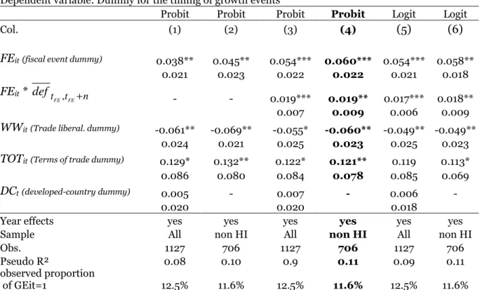
Table 5: Probit Estimates of Growth events

Dependent variable: Dummy for the timing of growth events

Probit Probit Probit Probit Logit Logit

Col. (1) (2) (3) (4) (5) (6)

FEit(fiscal event dummy) _{0.038** 0.045** 0.054*** 0.060*** 0.054*** 0.058**}

0.021 0.023 0.022 0.022 0.021 0.018 FEit * _, FE FE t t n def ₊ - - 0.019*** 0.019** 0.017*** 0.018** 0.007 0.009 0.006 0.009

WWit(Trade liberal. dummy) _{-0.061** -0.069** -0.055* -0.060** -0.049** -0.049**}

0.024 0.021 0.025 0.023 0.025 0.023

TOTit(Terms of trade dummy) _{0.129* 0.132** 0.122* 0.121** 0.119 0.113*}

0.086 0.080 0.084 0.078 0.085 0.069

DCt(developed-countrydummy) _{0.005 - 0.007 - 0.006 -}

0.020 0.020 0.018

Year effects yes yes yes yes yes yes

Sample All non HI All non HI All non HI

Obs. 1127 706 1127 706 1127 706

Pseudo R² 0.08 0.10 0.9 0.11 0.09 0.11

observed proportion

of GEit=1 12.5% 11.6% 12.5% 11.6% 12.5% 11.6%

Estimation by probit. Coefficients are marginal probabilities evaluated at the sample means. Numbers below coefficients are robust standard errors. See text for definition of variables. HI stands for “High Income” countries as defined by the World Bank, July 2007.

***, **, * indicates significant at the 1%, 5%, and 10% level respectively.

We allow for a five-year lag between a change in the underlying determinant and a growth event. The timing of the growth event is the three year window centered on the initiation dates.

Source: Authors’ computation, see Annex A.2.

Before commenting on the results, one should caution about the endogeneity problems, especially of the fiscal event dummy. It could be that in country-events when growth is anticipated to be unusually high, one might think that policy-makers would increase discretionary public spending (simultaneous bias if this increase occurs with a decreasing associated deficit). Unfortunately, we lack appropriate instruments, so the results should be interpreted accordingly. Cols. (1) and (2) in table 5 report the marginal coefficients corresponding to the estimation of (1) on the whole and on the “non high income” samples

respectively. Hence, the reported coefficients give directly the change in the probability that a growth event occurs for a discrete change of the

Col. (1) which reports estimates for all countries, shows that the coefficient associated with FEit is significantly positive (at the 5% level) implying that, on

average, a fiscal event increases the probability of experiencing a growth event in the five consecutive years by 3.8 percentage points. 22

Turning to the variable that captures the five years following economic reform (other than fiscal) through trade liberalization, WWit, surprisingly, the

coefficient is significantly negative. This coefficient was also negative but not significantly in HPR. However, this surprisingly negative coefficient does not necessarily contradict WW (2003) results since when they study the timing of the growth response to trade liberalization they find that, in the 3

pre-liberalization years, growth is slightly depressed and that, in the 3 years following liberalization, the effect is not significantly different from zero. However, an increase in growth becomes noticeable (of around 1.5 percentage point) after 4 years.23

As expected, we observe a strong conditional correlation between external shocks and the probability of a growth event: a large positive terms-of-trade shocks increases the probability of experiencing a growth event by 12.9

percentage points (significant at a 10% level). This confirms that the incidence of external shocks and, in particular, fluctuations in the terms of trade plays an important role. Finally, the high income dummy is not significantly different from zero so that when we limit our sample to “non high income” countries (see col. 2), coefficients remains very similar.

Recent literature assessing the effects of public expenditures on growth (e.g. Kneller et al., 2000, Bose et al., 2003, and Adam and Bevan, 2005) has emphasized the importance of incorporating the budget constraint. Here we check whether the impact of a fiscal event on the probability of a growth event is directly correlated with the level of the associated deficit by introducing the fiscal event dummy FEit interactively with its associated deficit/surplus level

, FE FE

t t n

def ₊ (t_FEbeing the date of the fiscal event, n=4).24

22

As argued in section 3, in “non-high” income countries, evidence suggests that fiscal policy typically pro-cyclical. Hence, if a growth event occurs in the year following a fiscal event, this should increase the deficit, weakening the probability of observing fiscal events followed by a growth event.

23 _{Remember that one of the conditions for a growth event in this paper is an increase in the} annual growth rate of per capita GDP of at least 2 pp. Hence, if we redefine the dummy WWit in order to capture the years [t+5 and more] after the trade liberalization instead of [t; t+4] as previously, we obtain a positive coefficient, though its value is not statistically significant. 24

Of course, the fiscal deficit/surplus situation is implicitly already taken into account as one of the conditions defining what we call a “Fiscal event” is that a deficit situation must improve.

Results reported in col. (3) and (4) show that the associated coefficient is

significantly positive (at 1% level) indicating that the marginal impact of a fiscal event depends on both coefficients (associated to FEit and FEit * _,

FE FE

t t n

def ₊ ).

This means that the probability of occurrence of a growth event in the 5 years following a fiscal event is greater the lower the associated fiscal deficit,

confirming the prima facie appropriateness of fiscal policy as a stabilizing

device. It would however, be premature to read into these results that there may not be a trade-off between the stabilization and growth objectives of fiscal

policy, since omitted variables correlated with the regressors are likely to influence these results. Coefficient values associated with WWit and TOTit

remain unchanged.

To ease interpretation, table 6 reports for a typical Low and Middle Income country, the impact of a fiscal event on the occurrence of a growth event for different values of the associated deficit/surplus. As indicated in the table, for a typical Low or Middle Income country and in the absence of a fiscal event in the five preceding years, the probability of a growth event is around 7.8%.25 _This

probability is quite similar in case of a fiscal event with an associated fiscal deficit equals to 3% of GDP (only 0.06 percentage point of difference).26 _The

probability of a growth event increases to 9.6% in case of a fiscal event in a deficit situation of 2% of GDP, and reaches 16.9% in a surplus situation of 1%, implying an increase in growth event probability of 9.1 percentage point

compared to the no-fiscal-event alternative. Remember that to be qualifying as fiscal event this deficit can not increase with public expenditure.

25 _{Based on results in table 5, col.(4) with 0} it

FE = , all other variables set at their sample mean. 26 _{Based on results in table 5, col.(4) with 1}

it

Table 6: Interpretation of Probit Model Results a/

Fiscal Event

associated with an average deficit of: No

Fiscal Event

-3% -2% -1% 0% 1%

Probability of occurrence of a growth

event in the 5 following years b/ 7.8% 7.8% 9.6% 11.8% 14.2% 16.9% Change in growth event probability

from a no fiscal event situation

0.06 pp 1.9 pp 4.0 pp 6.4 pp 9.1 pp

Note: pp stands for percentage points.

a/ Evaluation based on coefficients of the equation reported in column 4, table 5.

b/ Evaluation of _{0 1 1 , 2 3} 1 * FE FE t it it it it t t n t t FE FE def WW DC D φ α α α ₊ α α β − + + + + +     

∑

for different values of FEitand deft_FE,t_FE+n, all other variables evaluated at their sample mean,

φ

Source: Authors’ computation from table 5, col.4.

Finally, table 7 reports statistics of the predictive ability of this Probit model. It is customary to take a prediction rule with a threshold value is p* = 0.5, on the basis that we would predict a 1 if the model says a 1 is more likely than a zero :

1

it

GE = if the predicted probabilityφˆ > p*

However, because of the unbalanced sample with many more 0s than 1s, we set p* equal to the proportion of 1’s in the sample (which corresponds to the

average predicted probability in the sample).

Taking this criterion, table 7 suggests that the basic model as defined in table 5, column (4), successfully predicts 78% of the growth events (i.e. GEit=1) and

62.3% of total cases of no growth events (i.e. GEit=0). Hence, 64.2% of total

growth event observations are correctly predicted. Since this measure of

goodness of fit depends on the cutoff selected to classify the predicted GEit, one

Table 7: Prediction Accuracy of the Probit Model a/

Share of actual GEit predicted by the model

(share in total observation in parenthesis) actual GE=1 GE=0 GE=1 78.0% (9.1%) 37.7% (33.3%) GE=0 22.0% (2.5%) 62.3% (55.1%) P re d ic te d Total _{100.0% (11.6%) 100.0% (88.4%)} Correctly classified = 64.2%

a/ computation based on coefficients reported in column 4 in table 5 , cutoff =11.6% (value for determining whether an observation has a predicted positive outcome).

Source: Authors’ computation from table 5, col.4.

We carry out two robustness checks. First, as discussed above, we estimate a logit function (which has fatter tails and may be more appropriate for our sample with many zero values for the dependent variable). Results in columns (5) and (6) of table 5 show that the logit specification does not change the qualitative conclusions based on results in col. (3) and (4). Second, we change the definition of FEit with the dummy that takes the value of 1 at the date of the

fiscal event and during the 9 years following this date (instead of 4). This alternative, which gives more time for the effects of a fiscal event to have an impact on growth, does not alter qualitatively the estimates.

6. Conclusions

This paper constructs growth and primary spending expenditures (i.e.net of interest payments) “events” over the period 1972-2005 for 118 developing and 22 High Income OECD countries. Fiscal expenditures were compiled by Government function, and “events” were sought over 5-year rolling windows with a missing observation attributed if less than 4 out of 5 years of data were available. For the growth episodes, data was available for 87% of the potential of 6171 observations. For the fiscal episodes, data was available for 40% of the potential 4760 observations. In spite of more than half of the potential

observations missing for the construction of fiscal events, in the end, the search for events was based on a sufficiently large data base allowing for statistical tests.

Significant “events” were approximately constructed as follows (see section 3 and annex A.3 for details). For GDP per capita, acceleration in the average annual growth rate of 2 percentage point per annum (ppa) between any rolling 5-year window would qualify for a growth “event”. For fiscal expenditures (expressed in GDP%), an increase in the average growth rate of approximately 1 ppa that would not be accompanied by an aggravation of the (consolidated central government) fiscal deficit beyond 2% of GDP would likewise qualify for a fiscal “event”. The resulting benchmark constructed data set (merging both fiscal and growth databases) had 58 growth events and 95 fiscal events over a sample included 107 countries (84 developing countries) over 1977-2000 (1452 observations).

For this sample, the (unconditional) probability of occurrence of a fiscal event is about 10%, and, for a large range of parameter values for the selection of a “significant” event, the probability of a growth event once a fiscal event had occurred is in the 22%- 28% range. The probability of occurrence of a fiscal event is higher for the bottom half of the income distribution of countries, but the probability that this fiscal event is followed by a growth event is higher for the third quartiles, corresponding to middle income countries (which are largely in Latin America). Finally, the probability of a fiscal event not followed by a growth event is significantly higher for the Middle East and Africa region, prompting us to note that this result is coherent with the view (taken by the interim report presented to the Development Committee, 2006) that the success of a growth-oriented fiscal expenditure package hinges on the quality of the institutional environment.

For both “High income” and “Low and Middle Income” countries, fiscal events involve a shift towards education, health and Housing & Community

expenditures at the expense of defense, non-interest Public Services, and Transport & Communication expenditures, the shifts always being larger for developing countries, confirming more volatility (and probably a lesser

stabilization role of fiscal policy since the data cover a medium-term horizon). In particular, the Low and Middle Income country events indicate a much bigger cut in non-interest public services and in defense expenditures, the latter probably capturing countries entering a post-conflict situation.

Concentrating on the Low and Middle Income sample of 84 countries, the paper also investigates the differences in the pattern of functional expenditures for fiscal events followed by growth events compared to those not followed by a growth event. In addition to a significantly lower fiscal deficit for fiscal events followed by a growth event (which is partly an outcome of the way events were constructed), three other significant differences appear. First, fiscal events followed by growth events devote fewer resources to general public services. Second, fiscal events followed by a growth event are characterized by a growing share of transport and communication expenditure whereas the pattern is the opposite when the fiscal event is not followed by a growth event. Third, though the difference in means is not statistically significant, there is a higher growth in education expenditures when the fiscal event is followed by a growth event than when it is not.

This description of the anatomy of fiscal events and their relation to growth events is completed by statistical analysis where a few controlling factors are included in a probit estimate of growth events on fiscal events. On average, we find that a growth event is more likely to occur when surrounded by a fiscal event. Second, controlling for the growth-related effects of other reforms (captured by the Wacziarg-Welch indicator) and for favorable external conditions shocks (better terms-of-trade), we estimate that for a typical developing country, the probability of occurrence of a growth event in the five years following a fiscal event is increased as the associated fiscal deficit is limited.