HAL Id: inserm-00388967
https://www.hal.inserm.fr/inserm-00388967
Submitted on 23 Jul 2009HAL is a multi-disciplinary open access archive for the deposit and dissemination of sci-entific research documents, whether they are pub-lished or not. The documents may come from teaching and research institutions in France or abroad, or from public or private research centers.
L’archive ouverte pluridisciplinaire HAL, est destinée au dépôt et à la diffusion de documents scientifiques de niveau recherche, publiés ou non, émanant des établissements d’enseignement et de recherche français ou étrangers, des laboratoires publics ou privés.
and MEG.
Olivier David, Stefan Kiebel, Lee Harrison, Jérémie Mattout, James Kilner,
Karl Friston
To cite this version:
Olivier David, Stefan Kiebel, Lee Harrison, Jérémie Mattout, James Kilner, et al.. Dynamic causal modeling of evoked responses in EEG and MEG.. NeuroImage, Elsevier, 2006, 30 (4), pp.1255-72. �10.1016/j.neuroimage.2005.10.045�. �inserm-00388967�
Dynamic Causal Modeling of Evoked Responses in
EEG and MEG
Olivier David,* Stefan J. Kiebel, Lee M Harrison, Jérémie Mattout, James M. Kilner, Karl J. Friston
Wellcome Department of Imaging Neuroscience, Functional Imaging Laboratory, 12 Queen Square, London WC1N 3BG, UK
*
Present address: INSERM U594 Neuroimagerie Fonctionnelle et Métabolique, Université Joseph Fourier, CHU – Pavillon B – BP 217, 38043 Grenoble Cedex 09, France
Corresponding author: Stefan Kiebel
The Wellcome Dept. of Imaging Neuroscience, Institute of Neurology, UCL
12 Queen Square, London, UK WC1N 3BG Tel (44) 207 833 7478
Fax (44) 207 813 1420 Email [email protected]
Abstract
Neuronally plausible, generative or forward models are essential for understanding how event-related fields (ERFs) and potentials (ERPs) are generated. In this paper we present a new approach to modeling event-related responses measured with EEG or MEG. This approach uses a biologically informed model to make inferences about the underlying neuronal networks generating responses. The approach can be regarded as a neurobiologically constrained source reconstruction scheme, in which the parameters of the reconstruction have an explicit neuronal interpretation. Specifically, these parameters encode, among other things, the coupling among sources and how that coupling depends upon stimulus attributes or experimental context. The basic idea is to supplement conventional electromagnetic forward models, of how sources are expressed in measurement space, with a model of how source activity is generated by neuronal dynamics. A single inversion of this extended forward model enables inference about both the spatial deployment of sources and the underlying neuronal architecture generating them. Critically, this inference covers long-range connections among well-defined neuronal subpopulations.
In a previous paper, we simulated ERPs using a hierarchical neural-mass model that embodied bottom-up, top-down and lateral connections among remote regions. In this paper, we describe a Bayesian procedure to estimate the parameters of this model using empirical data. We demonstrate this procedure by characterizing the role of changes in cortico-cortical coupling, in the genesis of ERPs. In the first experiment, ERPs recorded during the perception of faces and houses were modeled as distinct cortical sources in the ventral visual pathway. Category-selectivity, as indexed by the face-selective N170, could be explained by category-specific differences in forward connections from sensory to higher areas in the ventral stream. We were able to quantify and make inferences about these effects using conditional estimates of connectivity. This allowed us to identify where, in the processing stream, category-selectivity emerged. In the second experiment we used an auditory oddball paradigm to show the mismatch negativity can be explained by changes in connectivity. Specifically, using Bayesian model selection, we assessed changes in backward connections, above and beyond changes in forward connections. In accord with theoretical predictions, there was strong evidence for learning-related changes in both forward and backward coupling. These examples show that category- or context-specific coupling among cortical regions can be assessed explicitly, within a mechanistic, biologically motivated inference framework.
Keywords: Electroencephalography, magnetoencephalography, neural networks, nonlinear dynamics, causal modeling, and Bayesian inference.
Introduction
Event-related fields (ERFs) and potentials (ERPs) have been used for decades as putative magneto- and electrophysiological correlates of perceptual and cognitive operations. However, the exact neurobiological mechanisms underlying their generation are largely unknown. Previous studies have shown that ERP-like responses can be reproduced by brief perturbations of model cortical networks (David et al., 2005; Jansen and Rit, 1995; Rennie et al., 2002). The goal of this paper was to demonstrate that biologically plausible dynamic causal models (DCMs) can explain empirical ERP phenomena. In particular, we show that changes in connectivity, among distinct cortical sources, are sufficient to explain stimulus- or set-specific ERP differences. Adopting explicit neuronal models, as an explanation of observed data, may afford a better understanding of the processes underlying event-related responses in magnetoencephalography (MEG) and electroencephalography (EEG).
Functional vs. effective connectivity
The aim of dynamic causal modeling (Friston et al., 2003) is to make inferences about the coupling among brain regions or sources and how that coupling is influenced by experimental factors. DCM uses the notion of effective connectivity, defined as the influence one neuronal system exerts over another. DCM represents a fundamental departure from existing approaches to connectivity because it employs an explicit generative model of measured brain responses that embraces their nonlinear causal architecture. The alternative to causal modeling is to simply establish statistical dependencies between activity in one brain region and another. This is referred to as functional connectivity. Functional connectivity is useful because it rests on an operational definition and eschews any arguments about how dependencies are caused. Most approaches in the EEG and MEG literature address functional connectivity, with a focus on dependencies that are expressed at a particular frequency of oscillations (i.e. coherence). See Schnitzler and Gross (2005) for a nice review. Recent advances have looked at nonlinear or generalized synchronization in the context of chaotic oscillators (e.g. Rosenblum et al 2002) and stimulus-locked responses of coupled oscillators (see Tass 2004). These characterizations often refer to phase-synchronization as a useful measure of nonlinear dependency. Another exciting development is the reformulation of coherence in terms of autoregressive models. A compelling example is reported in Brovelli et al (2004) who were able show that "synchronized beta oscillations bind multiple sensorimotor areas into a large-scale network during motor maintenance behavior and carry Granger causal influences from primary somatosensory and inferior posterior parietal cortices to motor cortex." Similar developments have been seen in functional neuroimaging with fMRI (e.g. Harrison et al., 2003; Roebroeck et al., 2005).
These approaches generally entail a two-stage procedure. First an electromagnetic forward model is inverted to estimate the activity of sources in the brain. Then, a post-hoc analysis is used to establish statistical dependencies (i.e. functional connectivity) using coherence, phase-synchronization, Granger influences or related analyses such as (linear} directed transfer functions and (nonlinear) generalized synchrony. DCM takes a very different approach and uses a forward model that explicitly includes long-range connections among neuronal sub-populations underlying measured sources. A single Bayesian inversion allows one to infer on parameters of the model (i.e. effective connectivity) that mediate functional
connectivity. This is like performing a biological informed source reconstruction with the added constraint that the activity in one source has to be caused by activity in other, in a biologically plausible fashion. This approach is much closer in sprit to the work of Robinson et al (2004) who show that "model-based electroencephalographic (EEG) methods can quantify neurophysiologic parameters that underlie EEG generation in ways that are complementary to and consistent with standard physiologic techniques." DCM also speaks to the interest in neuronal modeling of ERPs in specific systems. See for example Melcher and Kiang (1996), who evaluate a detailed cellular model of brainstem auditory evoked potentials (BAEP) and conclude "it should now be possible to relate activity in specific cell populations to psychophysical performance since the BAEP can be recorded in behaving humans and animals." See also Dau et al (2003). Although the models presented in this paper are more generic than those invoked to explain the BAEP, they share the same ambition of understanding the mechanisms of response generation and move away from phenomenological or descriptive quantitative EEG measures.
Dynamic causal modeling
The central idea behind DCM is to treat the brain as a deterministic nonlinear dynamical system that is subject to inputs, and produces outputs. Effective connectivity is parameterized in terms of coupling among unobserved brain states, i.e. neuronal activity in different regions. Coupling is estimated by perturbing the system and measuring the response. This is in contradistinction to established methods for estimating effective connectivity from neurophysiological time series, which include structural equation modeling and models based on multivariate autoregressive processes (Büchel and Friston, 1997; Harrison et al., 2003; McIntosh and Gonzalez-Lima, 1994). In these models, there is no designed perturbation and the inputs are treated as unknown and stochastic. Although the principal aim of DCM is to explain responses in terms of context-dependent coupling, it can also be viewed as a biologically informed inverse solution to the source reconstruction problem. This is because estimating the parameters of a DCM rests on estimating the hidden states of the modeled system. In ERP studies, these states correspond to the activity of the sources that comprise the model. In addition to biophysical and coupling parameters the DCMs parameters cover the spatial expression of sources at the sensor level. This means that inverting the DCM entails a simultaneous reconstruction of the source configuration and their dynamics.
Because DCMs are not restricted to linear or instantaneous systems they generally depend on a large number of free parameters. However, because it is biologically grounded, parameter estimation is constrained. A natural way to embody these constraints is within a Bayesian framework. Consequently, DCMs are estimated using Bayesian inversion and inferences about particular connections are made using their posterior or conditional density. DCM has been previously validated with functional magnetic resonance imaging (fMRI) time series (Friston et al., 2003; Riera et al., 2004). fMRI responses depend on hemodynamic processes that effectively low-pass filter neuronal dynamics. However, with ERPs this is not the case and there is sufficient information, in the temporal structure of evoked responses, to enable precise conditional identification of quite complicated DCMs. In this study, we use a model described recently (David et al., 2005) that embeds cortical sources, with several source-specific neuronal subpopulations, into hierarchical cortico-cortical networks.
This paper is structured as follows. In the theory section we review the neural mass model used to generate MEG/EEG-like evoked responses. This section summarizes David et al. (2005) in which more details about the generative model and associated dynamics can be found. The next section provides a brief review of Bayesian estimation, conditional inference and model comparison that are illustrated in the subsequent section. An empirical section then demonstrates the use of DCM for ERPs by looking at changes in connectivity that were induced, either by category-selective activation of different pathways in the visual system, or by sensory learning in an auditory oddball paradigm. This section concludes with simulations that demonstrate the face validity of the particular DCMs employed. Details about how the empirical data were acquired and processed will be found in an appendix.
THEORY
Intuitively, the DCM scheme regards an experiment as a designed perturbation of neuronal dynamics that are promulgated and distributed throughout a system of coupled anatomical nodes or sources to produce region-specific responses. This system is modeled using a dynamic input–state–output system with multiple inputs and outputs. Responses are evoked by deterministic inputs that correspond to experimental manipulations (i.e. presentation of stimuli). Experimental factors (i.e. stimulus attributes or context) can also change the parameters or causal architecture of the system producing these responses. The state variables cover both the neuronal activities and other neurophysiological or biophysical variables needed to form the outputs. In our case, outputs are those components of neuronal responses that can be detected by MEG/EEG sensors.
In neuroimaging, DCM starts with a reasonably realistic neuronal model of interacting cortical regions. This model is then supplemented with a forward model of how neuronal activity is transformed into measured responses; here MEG/EEG scalp averaged responses. This enables the parameters of the neuronal model (i.e., effective connectivity) to be estimated from observed data. For MEG/EEG data, the supplementary model is a forward model of electromagnetic measurements that accounts for volume conduction effects (Mosher et al., 1999). We first review the neuronal component of the forward model and then turn to the modality-specific measurement model.
A neural mass model
The majority of neural mass models of MEG/EEG dynamics have been designed to generate spontaneous rhythms (David and Friston, 2003; Jansen and Rit, 1995; Lopes da Silva et al., 1974; Robinson et al., 2001; Stam et al., 1999) and epileptic activity (Wendling et al., 2002). These models use a small number of state variables to represent the expected state of large neuronal populations, i.e. the neural mass. To date, event-related responses of neural mass models have received less attention (David et al., 2005; Jansen and Rit, 1995; Rennie et al., 2002). Only recent models have embedded basic anatomical principles that underlie extrinsic connections among neuronal populations:
The cortex has a hierarchical organization (Crick and Koch, 1998; Felleman and Van Essen, 1991), comprising forward, backward and lateral processes that can be understood from an anatomical and cognitive perspective (Engel et al., 2001). The direction of an anatomical projection is usually inferred from the laminar pattern of its origin and termination.
We have developed a hierarchical cortical model to study the genesis of ERFs/ERPs (David et al., 2005). This model is used here as a DCM. The neuronal part of the DCM comprises a network or graph of sources. In brief, each source is modeled with three neuronal subpopulations. These subpopulations are interconnected with intrinsic connections within each source. The sources are interconnected by extrinsic connections among specific subpopulations. The specific source and target subpopulations define the connection as forward, backward or lateral. The model is now reviewed in terms of the differential equations that embody its causal architecture.
Neuronal state equations
The model (David et al., 2005) embodies directed extrinsic connections among a number of sources, each based on the Jansen model (Jansen and Rit, 1995), using the connectivity rules described in (Felleman and Van Essen, 1991). These rules, which rest on a tri-partitioning of the cortical sheet into supra-, infra-granular layers and granular layer 4, have been derived from experimental studies of monkey visual cortex. We assume these rules generalize to other cortical regions (but see Smith and Poplin, 2001 for a comparison of primary visual and auditory cortices). Under these simplifying assumptions, directed connections can be classified as: (i) Bottom-up or forward connections that originate in agranular layers and terminate in layer 4. (ii) Top-down or backward connections that connect agranular layers. (iii) Lateral connections that originate in agranular layers and target all layers. These long-range or extrinsic cortico-cortical connections are excitatory and comprise the axonal processes of pyramidal cells.
The Jansen model (Jansen and Rit, 1995) emulates the MEG/EEG activity of a cortical source using three neuronal subpopulations. A population of excitatory pyramidal (output) cells receives inputs from inhibitory and excitatory populations of interneurons, via intrinsic connections (intrinsic connections are confined to the cortical sheet). Within this model, excitatory interneurons can be regarded as spiny stellate cells found predominantly in layer 4. These cells receive forward connections. Excitatory pyramidal cells and inhibitory interneurons occupy agranular layers and receive backward and lateral inputs. Using these connection rules, it is straightforward to construct any hierarchical cortico-cortical network model of cortical sources. See Figure 1.
Figure 1 about here
The ensuing DCM is specified in terms of its state equations and an observer or output equation
)
,
(
)
,
,
(
x
g
h
u
x
f
x
1where x are the neuronal states of cortical areas, u are exogenous inputs and h is the output of the system.
are quantities that parameterize the state and observer equations (see also below under ‘Prior assumptions’). The state equationsf
(
x
,
u
,
)
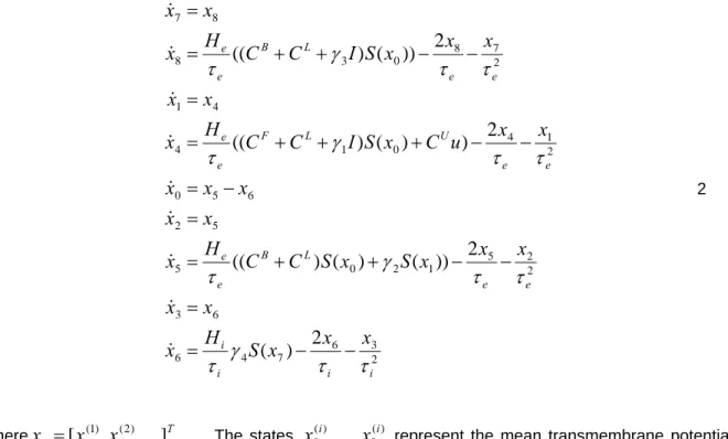
(Jansen and Rit 1995; David and Friston 2003; David et al 2005) for the neuronal states of multiple areas are12 3 6 7 4 6 6 3 2 2 5 1 2 0 5 5 2 6 5 0 2 1 4 0 1 4 4 1 2 7 8 0 3 8 8 7
2
)
(
2
))
(
)
(
)
((
2
)
)
(
)
((
2
))
(
)
((
i i i i e e L B e e e e U L F e e e e L B e ex
x
x
S
H
x
x
x
x
x
x
S
x
S
C
C
H
x
x
x
x
x
x
x
x
u
C
x
S
I
C
C
H
x
x
x
x
x
x
S
I
C
C
H
x
x
x
2where
x
j
[
x
(j1),
x
(j2),
]
T. . The statesx
0(i),
,
x
8(i) represent the mean transmembrane potentials and currents of the three subpopulations in the i-th source. The state equations specify the rate of change of voltage as a function of current and specify how currents change as a function of voltage and current. Figure 1 depicts the states by assigning each subpopulation to a cortical layer. For schematic reasons we have lumped superficial and deep pyramidal units together, in the infra-granular layer. The matricesL B F
C
C
C
,
,
encode forward, backward and lateral extrinsic connections respectively. From Eq.2 and Figure 1 it can be seen that the state equations embody the connection rules above. For example, extrinsic connections mediating changes in mean excitatory [depolarizing] currentx
8, in the supragranular layer, are restricted to backward and lateral connections. The depolarisation of pyramidal cellsx
0
x
2
x
3 represents a mixture of potentials induced by excitatory and inhibitory [depolarizing and hyperpolarizing] currents respectively. This pyramidal potential is the presumed source of observed MEG/EEG signals.The remaining constants in the state equation pertain to two operators, on which the dynamics rest. The first transforms the average density of pre-synaptic inputs into the average postsynaptic membrane potential. This transformation is equivalent to a convolution with an impulse response or kernel,
1
Propagation delays
on the connections have been omitted for clarity, here and in Figure 1. See Appendix A.1 for details of how delays are incorporated.
0
0
0
)
exp(
)
(
t
t
t
t
H
t
p
e e e e
3where subscript “e” stands for “excitatory”. Similarly, the subscript “i” is used for inhibitory synapses.
H
controls the maximum post-synaptic potential and
represents a lumped rate constant. The second operator S transforms the potential of each subpopulation into firing rate, which is the input to other subpopulations. This operator is assumed to be an instantaneous sigmoid nonlinearity
2
1
exp
1
1
)
(
rx
x
S
4where
r
.
56
determines its form. Figure 2 shows examples of these synaptic kernels and sigmoid functions. Interactions, among the subpopulations, depend on the constants
1,2,3,4, which control the strength of intrinsic connections and reflect the total number of synapses expressed by each subpopulation. A DCM, at the neuronal level, obtains by coupling sources with extrinsic connections as described above. A typical three-source DCM is shown in Figure 3. See David and Friston 2003 and David et al 2005 for further details.Figure 2 about here
Event-related input and ERP-specific effects
To model event-related responses, the network receives inputs via input connections
C
U. These connections are exactly the same as forward connections and deliver inputs u to the spiny stellate cells in layer 4. In the present context, inputs u model afferent activity relayed by subcortical structures and is modeled with two components.
(
,
,
)
cos(
2
(
1
)
)
)
(
t
b
t
1 2i
t
u
c i
5The first is a gamma density function
(
,
,
)
exp(
2)
(
1)
1 2 2 1 1 1
t
t
t
b
with shape and scaleconstants
1 and
2 (see Table 1). This models an event-related burst of input that is delayed (by
1
2 sec) with respect to stimulus onset and dispersed by subcortical synapses and axonal conduction. Being a density function, this component integrates to unity over peristimulus time. The second component is a discrete cosine set modeling systematic fluctuations in input, as a function of peristimulus time. In our implementation peristimulus time is treated as a state variable, allowing the input to be computed explicitly during integration.Critically, the event-related input is exactly the same for all ERPs. This means the effects of experimental factors are mediated through ERP-specific changes in connection strengths. This models experimental effects in terms of differences in forward, backward or lateral connections that confer a selective sensitivity on each source, in terms of its response to others. The experimental or ERP-specific effects are modeled by coupling gains ijk L ij L ijk ijk B ij B ijk ijk F ij F ijk
G
C
C
G
C
C
G
C
C
6Here,
C
ij encodes the strength of the latent connection to the i-th source from the j-th andG
ijk encodes its k-th specific gain. By convention, we set the gain of the first ERP to unity, so that subsequent ERP-specific effects are relative to the first2. The reason we model experimental effects in terms of gain, as opposed to additive effects, is that by construction, connections are always positive. This is assured; provided the gain is also positive.The important point here is that we are explaining experimental effects, not in terms of differences in neuronal responses, but in terms of the neuronal architecture or coupling generating those responses. This is a fundamental departure from classical approaches, which characterize experimental effects descriptively, at the level of the states (e.g. a face-selective difference in ERP amplitude around 170ms). DCM estimates these response differentials but only as an intermediate step in the estimation of their underlying cause; namely changes in coupling.
Eq.2 defines the neuronal component of the DCM. These ordinary differential equations can be integrated using standard techniques (see Appendix A.2 and Kloeden and Platen, 1999) to generate pyramidal depolarisations, which enters the observer function to generate the predicted MEG/EEG signal.
Figure 3 about here
Observation equations
The dendritic signal of the pyramidal subpopulation of the i-th source
x
0(i) is detected remotely on the scalp surface in MEG/EEG. The relationship between scalp data and pyramidal activity is linear0
)
,
(
x
LKx
g
h
72
In fact, in our implementation, the coupling gain is a function of any set of explanatory variables encoded in a design matrix, which can contain indicator variables or parametric variables. For simplicity, we limit this paper to categorical (ERP-specific) effects.
where L is a lead-field matrix (i.e., forward electromagnetic model), which accounts for passive conduction of the electromagnetic field (Mosher et al., 1999). If the spatial properties (orientation and position) of the source are known, then the lead-field matrix L is also known. In this case,
K
diag
(
K)
is a leading diagonal matrix, which controls the contribution
iKof pyramidal depolarisation to the i-th source density. If the orientation is not known thenL
[
L
x,
L
y,
L
z]
encodes sensor responses to orthogonal dipoles and the source orientation can be derived from the contribution to these orthogonal components encoded byK
[
diag
(
xK),
diag
(
yK),
diag
(
zK)]
T . In this paper, we assume a fixed orientation for multiple dipoles for each source (see Appendix A.3) but allow the orientation to be parallel or anti-parallel (i.e.
K can be positive or negative). The rationale for this is that the direction of current flow induced by pyramidal cell depolarisation depends on the relative density of synapses proximate and distal to the cell body.Dimension reduction
For computational reasons, it is sometimes expedient to reduce the dimensionality of the sensor data, while retaining the maximum amount of information. This is assured by projecting the data onto a subspace defined by its principal eigenvectors E
E
EL
L
Ey
y
8Because this projection is orthonormal, the independence of the projected errors is preserved and the form of the error covariance components of the observation model remains unchanged. In this paper we reduce the sensor space to three dimensions (see appendix A.4).
The observation model
In summary, our DCM comprises a state equation that is based on neurobiological heuristics and an observer based on an electromagnetic forward model. By integrating the state equation and passing the ensuing states through the observer we generate a predicted measurement. This corresponds to a generalized convolution of the inputs to generate an output
h
(
)
. This generalized convolution furnishes an observation model for the vectorised data3 y and the associated likelihood)
)
(
),
)
(
(
(
)
,
(
)
)
(
(
V
diag
X
h
vec
N
y
p
X
h
vec
y
X X
93
Measurement noise
is assumed to be zero mean and independent over channels, i.e.V
diag
Cov
(
)
(
)
, where
is an unknown vector of channel-specific variances. V represents the errors temporal autocorrelation matrix, which we assume is the identity matrix. This is tenable because we down-sample the data to about 8-ms. Low frequency noise or drift components are modeled by X, which is a block diagonal matrix with a low-order discrete cosine set for each ERP and channel. The order of this set can be determined by Bayesian model selection (see below). In this paper we used three components for the first study and four for the second. The first component of a discrete cosine set is simply a constant.This model is fitted to data using Variational Bayes (see below). This involves maximizing the variational free energy with respect to the conditional moments of the free parameters
. These parameters specify the constants in the state and observation equations above. The parameters are constrained by a prior specification of the range they are likely to lie in (Friston et al., 2003). These constraints, which take the form of a prior densityp
(
)
, are combined with the likelihoodp
(
y
|
,
)
, to form a posterior density)
(
)
,
|
(
)
,
|
(
y
p
y
p
p
according to Bayes rule. It is this posterior or conditional density we want to approximate. Gaussian assumptions about the errors in Eq.9 enable us to compute the likelihood from the prediction error. The only outstanding quantities we require are the priors, which are described next.Prior assumptions
Here we describe how the constant terms, defining the connectivity architecture and dynamical behavior of the DCM, are parameterized and our prior assumptions about these parameters. Priors have a dramatic impact on the landscape of the objective function to be extremised: precise prior distributions ensure that the objective function has a global minimum that can be attained robustly. Under Gaussian assumptions, the prior distribution
p
(
i)
of the I-th parameter is defined by its mean and variance. The mean corresponds to the prior expectation. The variance reflects the amount of prior information about the parameter. A tight distribution (small variance) corresponds to precise prior knowledge.Critically, nearly all the constants in the DCM are positive. To ensure positivity we estimate the log of these constants under Gaussian priors. This is equivalent to adopting a log-normal prior on the constants per se. For example, the forward connections are re-parameterized as
C
ijF
exp(
θ
ijF)
, wherep
(
ijF)
N
(
,
v
)
.
andv
are the prior expectation and variance ofln
C
ijF
θ
ijF . A relatively tight or informative log-normal prior obtains whenv
161 . This allows for a scaling around the prior expectation of up to a factor of two.Relatively flat priors, allowing for an order of magnitude scaling, correspond to
v
21. The ensuinglognormal densities are shown in Figure 4 for a prior expectation of unity (i.e.
0
). Table 1 about hereThe parameters of the state equation can be divided into five subsets: (i) extrinsic connection parameters, which specify the coupling strengths among areas and (ii) intrinsic connection parameters, which reflect our knowledge about canonical micro-circuitry within an area. (iii) Conduction delays. (iv) Synaptic parameters controlling the dynamics within an area and (v) input parameters, which control the subcortical delay and dispersion of event-related responses. Table 1 shows how the constants of the state equation are re-parameterized in terms of
. It can be seen that we have adopted relatively uninformative priors on the extrinsic couplingv
21 and tight priors for the remaining constants16 1
v
. Some parameters (intrinsic connections and inhibitory synaptic parameters) have infinitely tight priors and are fixed at their prior expectation. This is because changes in these parameters and the excitatory synaptic parameters are almost redundant, in terms of system responses. The priors in Table 1 conform to the principle that the parameters we want to make inferences about, namely extrinsic connectivity, should have relatively flat priors. This ensures that the evidence in the data constrains the posterior or conditional density in an informative and useful way. In what follows we review briefly our choice of prior expectations (see David et al., 2005 for details).Figure 4 about here
Prior expectations
Extrinsic parameters comprise the matrices
{
F,
B,
L,
G,
U}
that control the strength of connections and their gain. The prior expectations for forward, backward, and lateral;ln
32
,ln
16
and4
ln
respectively, embody our prior assumption that forward connections exert stronger effects than backward or lateral connections. The prior expectation of
ijkG is zero, reflecting the assumption that, in the absence of evidence to the contrary, experimental effects are negligible and the trial-specific gain ise
0
1
. In practice, DCMs seldom have a full connectivity and many connections are disabled by setting their prior toN
(
,
0
)
. This is particularly important for the input connections parameterized by
iU, which generally restrict inputs to one or two cortical sources.We fixed the values of intrinsic coupling parameters as described in (Jansen and Rit, 1995). Inter-laminar conduction delays were fixed at 2 ms and inter-regional delays had a prior expectation of 16 ms. The priors on the synaptic parameters for the I-th area
{
i,
iH}
constrain the lumped time-constant and relative postsynaptic density of excitatory synapses respectively. The prior expectation for the lumped time constant was 8-ms. This may seem a little long but it has to accommodate, not only dynamics within dendritic spines, but integration throughout the dendritic tree.Priors on the input parameters
{
1,
2,
1c,
,
8c}
were chosen to give an event-related burst, with a dispersion of about 32 ms, 96 ms after trial onset. The input fluctuations were relatively constrained with a prior on their coefficients ofp
(
ic)
N
(
0
,
1
)
. We used the same prior on the contribution of depolarisationto source dipoles
p
(
iK)
N
(
0
,
1
)
. This precludes large values explaining away ERP differences in terms of small differences at the cortical level (Grave de Peralta Menendez and Gonzalez-Andino, 1998). Finally, the coefficients of the noise fluctuations were unconstrained, with flat priorsp
(
X)
N
(
0
,
)
.Summary
In summary, a DCM is specified in through its priors. These are used to specify (i) how regions are interconnected, (ii) which regions receive subcortical inputs, and (iii) which cortico-cortical connections change with the levels of experimental factors. Usually, the most interesting questions pertain to changes in cortico-cortical coupling that explain differences in ERPs. These rest on inferences about the coupling gains
G ijk
. This section has covered the likelihood and prior densities necessary for conditional estimation. For each model, we require the conditional densities of two synaptic parameters per source{
i,
iH}
, ten input parameters{
1,
2,
1c,
,
8c}
and the extrinsic coupling parameters, gains and delays}
,
,
,
,
,
{
F
B
L
G
U
. The next section reviews conditional estimation of these parameters, inference and model selection.BAYESIAN INFERENCE AND MODEL COMPARISON
Estimation and inference
For a given DCM, say model m; parameter estimation corresponds to approximating the moments of the posterior distribution given by Bayes rule
)
|
(
)
,
(
)
,
|
(
)
,
|
(
m
y
p
m
p
m
y
p
m
y
p
10The estimation procedure employed in DCM is described in (Friston, 2002). The posterior moments (conditional mean
and covariance
) are updated iteratively using Variational Bayes under a fixed-form Laplace (i.e. Gaussian) approximation to the conditional densityq
(
)
N
(
,
)
. This can be regarded as an Expectation-Maximization (EM) algorithm that employs a local linear approximation of Eq.9 about the current conditional expectation. The E-step conforms to a Fisher-scoring scheme (Press et al., 1992) that performs a descent on the variational free energyF
(
q
,
,
m
)
with respect to the conditional moments. In the M-Step, the error variances
are updated in exactly the same way. The estimation scheme can be summarized as follows:)
,
|
(
ln
)
,
(
)
,
(
)
,
,
|
(
||
(
)
|
(
ln
)
,
,
|
(
ln
)
(
ln
)
,
,
(
)
,
(
max
)
,
,
(
min
)
,
,
(
min
Step
Step
m
y
p
m
L
m
L
m
y
p
q
D
m
p
m
y
p
q
m
q
F
m
L
m
q
F
m
q
F
q
q q
M
E
11Note that the free energy is simply a function of the log-likelihood and the log-prior for a particular DCM and
)
(
q
.q
(
)
is the approximation to the posterior densityp
(
|
y
,
,
m
)
we require. The E-step updates the moments ofq
(
)
(these are the variational parameters
and
) by minimizing the variational free energy. The free energy is the divergence between the real and approximate conditional density minus the likelihood. This means that the conditional moments or variational parameters maximize the log-likelihoodL
(
,
m
)
while minimising the discrepancy between the true and approximate conditional density. Because the divergence does not depend on the covariance parameters, minimizing the free energy in the M-step is equivalent to finding the maximum likelihood estimates of the covariance parameters. This scheme is identical to that employed by DCM for fMRI, the details of which can be found in Friston (2002) and Friston et al (2003).Conditional inference
Inference on the parameters of a particular model proceeds using the approximate conditional or posterior density
q
(
)
. Usually, this involves specifying a parameter or compound of parameters as a contrastc
T
. Inferences about this contrast are made using its conditional covariancec
T
c
. For example, one can compute the probability that any contrast is greater than zero or some meaningful threshold, given the data. This inference is conditioned on the particular model specified. In other words, given the data and model, inference is based the probability that a particular contrast is bigger than a specified threshold. In some situations one may want to compare different models. This entails Bayesian model comparison.Model comparison and selection
Different models are compared using their evidence (Penny et al., 2004). The model evidence is
m
p
m
d
y
p
m
y
p
(
|
)
(
|
,
)
(
|
)
. 12The evidence can be decomposed into two components: an accuracy term, which quantifies the data fit, and a complexity term, which penalizes models with a large number of parameters. Therefore, the evidence
embodies the two conflicting requirements of a good model, that it explains the data and is as simple as possible. In the following, we approximate the model evidence for model m, with the free energy after convergence. This rests on the assumption that
has a point mass at its maximum likelihood estimate (equivalent to its conditional estimate under flat priors); i.e.,ln
p
(
y
|
m
)
ln
p
(
y
|
,
m
)
L
(
,
m
)
. After convergence the divergence is minimized and)
,
,
(
)
,
(
)
|
(
ln
p
y
m
L
m
F
q
m
13See Eq.11. The most likely model is the one with the largest log-evidence. This enables Bayesian model selection. Model comparison rests on the likelihood ratio of the evidence for two models. This ratio is the Bayes factor
B
ij. For models i and j)
|
(
ln
)
|
(
ln
ln
B
ij
p
y
m
i
p
y
m
j
14Conventionally, strong evidence in favor of one model requires the difference in log-evidence to be three or more. We have now covered the specification, estimation and comparison of DCMs. In the next section we will illustrate their application to real data using two important examples of how changes in coupling can explain ERP differences.
EMPIRICAL STUDIES
In this section we illustrate the use of DCM by looking at changes in connectivity induced in two different ways. In the first experiment we recorded ERPs during the perception of faces and houses. It is well-known that the N170 is a specific ERP correlate of face perception (Allison et al., 1999). The N170 generators are thought to be located close to the lateral fusiform gyrus, or Fusiform Face Area (FFA). Furthermore, the perception of houses has been shown to activate the Parahippocampal Place Area (PPA) using fMRI (Aguirre et al., 1998; Epstein and Kanwisher, 1998; Haxby et al., 2001; Vuilleumier et al., 2001). In this example, differences in coupling define the category-selectivity of pathways that are accessed by different categories of stimuli. A category-selective increase in coupling implies that the region receiving the connection is selectively more sensitive to input elicited by the stimulus category in question. This can be attributed to a functional specialization of receptive field properties and processing dynamics of the region receiving the connection. In the second example, we used an auditory oddball paradigm, which produces mismatch negativity (MMN) or P300 components in response to rare stimuli, relative to frequent (Debener et al., 2002; Linden et al., 1999). In this paradigm, we attribute changes in coupling to plasticity underlying the perceptual learning of frequent or standard stimuli.
In the category-selectivity paradigm there are no necessary changes in connection strength; pre-existing differences in responsiveness are simply disclosed by presenting different stimuli. This can be modeled by differences in forward connections. However, in the oddball paradigm, the effect only emerges once
standard stimuli have been learned. This implies some form of perceptual or sensory learning. We have presented a quite detailed analysis of perceptual learning in the context of empirical Bayes (Friston 2003). We concluded that the late components of oddball responses could be construed as a failure to suppress prediction error, after learning the standard stimuli. Critically, this theory predicts that learning-related plasticity should occur in backward connections generating the prediction, which are then mirrored in forward connections. In short, we predicted changes in forward and backward connections when comparing ERPs for standard and oddball stimuli.
In the first example, we are interested in where category-selective differences in responsiveness arise in a forward processing stream. Backward connections are probably important in mediating this selectivity but exhibit no learning-related changes per se. We use inferences based on the conditional density of coupling-gain, when comparing face and house ERPs, to address this question. In the second example, our question is more categorical in nature; namely, are changes in backward and lateral connections necessary to explain ERPs differences between standards and oddballs, relative to changes in forward connections alone? We illustrate the use of Bayesian model comparison to answer this question. See Appendices A.3 and A.4 for a description of the data acquisition, lead-field specification and preprocessing.
Category-selectivity: effective connectivity in the ventral visual pathway
ERPs elicited by brief presentation of faces and houses were obtained by averaging trials over three successive 20-minute sessions. Each session comprised 30 blocks of faces or houses only. Each block contained 12 stimuli presented every 2.6s for 400ms. The stimuli comprised 18 neutral faces and 18 houses, presented in grayscale. To maintain attentional set, the subject was asked to perform a one-back task, i.e. indicate, using a button press, whether or not the current stimulus was identical to the previous.
As reported classically, we observed a stronger N170 component during face perception in the posterior temporal electrodes. However, we also found other components, associated with house perception, which were difficult to interpret on the basis of scalp data. It is generally thought that face perception is mediated by a hierarchical system of bilateral regions (Haxby et al., 2002). (i) A core system, of occipito-temporal regions in extrastriate visual cortex (inferior occipital gyrus, IOG; lateral fusiform gyrus or face area, FFA; superior temporal sulcus, STS), that mediates the visual analysis of faces, and (ii) an extended system for cognitive functions. This system (intra-parietal sulcus; auditory cortex; amygdala; insula; limbic system) acts in concert with the core system to extract meaning from faces. House perception has been shown to activate the Parahippocampal Place Area (PPA) (Aguirre et al., 1998; Epstein and Kanwisher, 1998; Haxby et al., 2001; Vuilleumier et al., 2001). In addition, the Retrosplenial Cortex (RS) and the lateral occipital gyrus are more activated by houses, compared to faces (Vuilleumier et al., 2001). Most of these regions belong to the ventral visual pathway. It has been argued that the functional architecture of the ventral visual pathway is not a mosaic of category-specifics modules, but rather embodies a continuous representation of information about object attributes (Ishai et al., 1999).
DCM specification
We tested whether differential propagation of neuronal activity through the ventral pathway is sufficient to explain the differences in measured ERPs. On the basis of a conventional source localization (see Appendix A.3) and previous studies (Allison et al., 1999; Haxby et al., 2001; Haxby et al., 2002; Ishai et al., 1999; Vuilleumier et al., 2001), we specified the following DCM (see Figure 5): bilateral occipital regions close to the calcarine sulcus (V1) received subcortical visual inputs. From V1 onwards, the pathway for house perception was considered to be bilateral and to hierarchically connect RS and PPA using forward and backward connections. The pathway engaged by face perception was restricted to the right hemisphere and comprised connections from V1 to IOG, which projects to STS and FFA. In addition, bilateral connections were included, between STS and FFA, as suggested in (Haxby et al., 2002). These connections constituted our DCM mediating ERPs to houses and faces. This DCM is constrained anatomically by the number and location of regional sources that accounted for most of the variance in sensor-space (see Appendix A.4). Face- or house-specific ERP components were hypothesized to arise from selective, stimulus-bound, activation of forward pathways. To identify these category-selective streams we allowed the forward connections, in the right hemisphere, to change with category. Our hope was that these changes would render PPA more responsive to houses while the FFA and STS would express face-selective responses.
Figure 6 about here
Conditional inference
The results are shown in Figure 6, in terms of predicted cortical responses and coupling parameters. Using this DCM we were able to replicate the functional anatomy, disclosed by the above fMRI studies: the response in PPA was more marked when processing houses versus faces. This was explained, in the model, by an increase of forward connectivity in the medial ventral pathway from RS to PPA. This difference corresponded to a coupling-gain of over five-fold. Conversely, the model exhibited a much stronger response in FFA and STS during face perception, as suggested by the Haxby model (Haxby et al., 2002). This selectivity was due to an increase in coupling from IOG to FFA and from IOG to STS. The face-selectivity of STS responses was smaller than in the FFA, the latter mediated by an enormous gain of about nine-fold (
1
0
.
11
9
.
09
) in sensitivity to inputs from IOG. The probability, conditional on the data and model, that changes in forward connections to the PPA, STS and FFA, were greater than zero, was essentially 100% in all cases. The connections from V1 to IOG showed no selectivity. This suggests that category-selectivity emerges downstream from IOG, at a fairly high level. Somewhat contrary to expectations (see Vuilleumier et al., 2001), the coupling from V1 to RS showed a mild face-selective bias, with an increase of about 80% (1
0
.
55
1
.
82
).Note how the ERPs of each source are successively transformed and delayed from area to area. This reflects the intrinsic transformations within each source, the reciprocal exchange of signals between areas and the ensuing conduction delays. These transformations are mediated by intrinsic and extrinsic connections and are the dynamic expression of category selectivity in this DCM.
The conditional estimate of the subcortical input is also shown in Figure 6. The event-related response input was expressed about 96 ms after stimulus onset. The accuracy of the model is evident in the left panel of Figure 6, which shows the measured and predicted responses in sensor space, after projection onto their three principal eigenvectors.
Auditory oddball: effective connectivity and sensory learning
Auditory stimuli, 1000 or 2000 Hz tones with 5 ms rise and fall times and 80 ms duration, were presented binaurally for 15 minutes, every 2 seconds in a pseudo-random sequence. 2000-Hz tones (oddballs) occurred 20% of the time (120 trials) and 1000-Hz tones (standards) 80% of the time (480 trials). The subject was instructed to keep a mental record of the number of 2000-Hz tones.
Late components, characteristic of rare events, were seen in most frontal electrodes, centered on 250 ms to 350 ms post-stimulus. As reported classically, early components (i.e. the N100) were almost identical for rare and frequent stimuli. Using an conventional reconstruction algorithm (see Appendix A.3) cortical sources were localized symmetrically along the medial part of the upper bank of the Sylvian fissure, in the right middle temporal gyrus, left medial and posterior cingulate, and bilateral orbitofrontal cortex (see insert in Figure 7). These locations are in good agreement with the literature: Sources along the upper bank of the Sylvian fissure can be regarded as early auditory cortex, although they are generally located in the lower bank of the Sylvian fissure (Heschls gyrus). Primary auditory cortex has major inter-hemispheric connections through the corpus callosum. In addition, these areas project to temporal and frontal lobes following different streams (Kaas and Hackett, 2000; Romanski et al., 1999). Finally, cingulate activations are often found in relation to oddball tasks, either auditory or visual (Linden et al., 1999).
Figure 7 about here
DCM specification
Using these sources and prior knowledge about the functional anatomy of the auditory system, we constructed the following DCM (Figure 7): an extrinsic (thalamic) input entered bilateral primary auditory cortex (A1) which was connected to ipsilateral orbitofrontal cortex (OF). In the right hemisphere, an indirect forward pathway was specified from A1 to OF through the superior temporal gyrus (STG). All these connections were reciprocal. At the highest level in the hierarchy, OF and left posterior cingulate cortex (PC) was laterally and reciprocally connected.
Model comparison
Given these nodes and their connections, we created four DCMs that differed in terms of which connections could show putative learning-related changes. The baseline model precluded any differences between standard and oddball trials. The remaining four models allowed changes in forward F, backward B, forward and backward FB and all connections FBL, with the primary auditory sources. The results of a Bayesian model comparison (Penny et al. 2004) are shown in Figure 7, in terms of the respective log-evidences (referred to the baseline model with no coupling changes). There is very strong evidence for conjoint
changes in backward and lateral connections, above and beyond changes in forward or backward connections alone. The FB model supervenes over the FBL model that was augmented with plasticity in lateral connections between A1. This is interesting because the FBL model had more parameters, enabling a more accurate modeling of the data. However, the improvement in accuracy did not meet the cost of increasing the model complexity and the log-evidence fell by 4.224. This means there is strong evidence for the FB model, in relation to the FBL model. Put more directly, the data are e4.224 68.3 times more likely to have been generated by the FB model than the FBL model. The results of this Bayesian model comparison suggest the theoretical predictions were correct.
Other theoretical perspectives suggest that the MMN can be explained simply by an adaptation to standard stimuli that may only involve intrinsic connections (see, for example, Ulanovsky et al 2003). This hypothesis could be tested using stimulus-specific changes in intrinsic connections and model selection to assess whether the data are explained better by changes in intrinsic connectivity, extrinsic connectivity or both. We will pursue this in a future communication.
Figure 8 about here
Conditional inference
The conditional estimates and posterior confidences for the FB model are shown in Figure 8 and reveal a profound increase, for rare events, in all connections. We can be over 95% confident these connections increased. As above, these confidences are based on the conditional density of the coupling-gains. The conditional density of a contrast, averaging over all gains in backward connections, is shown in Figure 9. We can be 99.9% confident this contrast is greater than zero. The average is about one, reflecting a gain of about
e
1
2
.
7
, i.e., more than a doubling of effective connectivity.These changes produce a rather symmetrical series of late components, expressed to a greater degree, but with greater latency, at hierarchically higher levels. In comparison with the visual paradigm above, the subcortical input appeared to arrive earlier, around 64 ms after stimulus onset. The remarkable agreement between predicted and observed channel responses is seen in the left panel, again shown as three principal eigenvariates.
In summary, this analysis suggests that a sufficient explanation for mismatch responses is an increase in forward and backward connections with primary auditory cortex. This results in the appearance of exuberant responses after the N100 in A1 to unexpected stimuli. This could represent a failure to suppress prediction error, relative to predictable or learned stimuli, which can be predicted more efficiently.
Figure 9 about here
In this introductory paper we have focussed on the motivation and use of DCM for ERPs. We hope to have established its construct validity in relation to other neurobiological constructs (i.e., the functional anatomy of category-selectivity as measured by fMRI and predictive coding models of perceptual learning). There are many other aspects of validity that could be addressed and will be in future communications. Here, we briefly establish face validity (the procedure estimates what it is supposed to) of the particular DCM described above. This was achieved by integrating the DCM and adding noise to simulate responses of a system with known parameters. Face validity requires the true values to lie within the 90% confidence intervals of the conditional density. We performed two sets of simulations. The first involved changing one of the parameters (the gain in the right A1 to STG connection) and comparing the true values with the conditional densities. The second used the same parameters but different levels of noise (i.e., different variance parameters). In short, we reproduced our empirical study but with known changes in connectivity. We then asked whether the estimation scheme could recover the true values, under exactly the same conditions entailed by the empirical studies above.
The first simulations used the conditional estimates from the FB model of the auditory oddball paradigm. The gain on the right A1 to STG connection was varied from one half to two, i.e.
62G was increased from2
ln
toln
2
in 16 steps. The models were integrated to generate responses to the estimated subcortical input and Gaussian noise was added using the empirical ReML variance estimates. The conditional densities of the parameters were estimated from these simulated data in exactly the same way as for the empirical data. Note that this is a more stringent test of face validity than simply estimating connection strengths: we simulated an entire paradigm and tried to recover the changes or gain in coupling subtending the oddball effect. The results of these simulations are shown in Figure 10 for the connection that changed (right A1 to STG: upper panel) and for one that did not (right OF to A1: lower panel). In both cases the true value fell within the 90% confidence intervals. This speaks to the sensitivity (upper panel) and specificity (lower panel) of conditional inferences based on this model.Figure 10 about here
The results of the second simulations are shown in Figure 11. Here we repeated the above procedure but changed the variance parameters, as opposed to a coupling parameter. We simply scaled all the error variances by a factor that ranged from a half to two, in 16 steps. Figure 11 shows that the true value (of the right A1 to STG connection) again fell well within the 90% conditional confidence intervals, even for high levels of noise. These results also speak to the characteristic shrinkage of conditional estimators: Note that the conditional expectation is smaller than the true value at higher noise levels. The heuristic, behind this effect, is that noise or error induces a greater dependency on the priors and a consequent shrinkage of the conditional expectation to the prior expectation of zero. Having said this, the effect of doubling error variance in this context is unremarkable.
Discussion
We have described a Bayesian inference procedure in the context of DCM for ERPs. DCMs are used in the analysis of effective connectivity to provide posterior or conditional distributions. These densities can then be used to assess changes in effective connectivity caused by experimental manipulations. These inferences, however, are contingent on assumptions about the architecture of the model, i.e., which regions are connected and which connections are modulated by experimental factors. Bayesian model comparison can be used to adjudicate among competing models, or hypotheses, as demonstrated above. In short, DCMs can be used to test hypotheses about the functional organization of macroscopic brain activity. In neuroimaging, DCMs have been applied to fMRI data (Friston et al., 2003; Penny et al., 2004; Riera et al., 2004). We have shown that MEG/EEG event-related responses can also be subject to DCM.
The approach can be regarded as a neurobiologically constrained source reconstruction scheme, in which the parameters of the reconstruction have an explicit neuronal interpretation, or as a characterization of the causal architecture of the neuronal system generating responses. We hope to have shown that it is possible to test mechanistic hypotheses in a more constrained way than classical approaches because the prior assumptions are physiologically informed.
Our DCMs use a neural mass model that embodies long-range cortico-cortical connections by considering forward, backward and lateral connections among remote areas (David et al., 2005). This allows us to embed neural mechanisms generating MEG/EEG signals that are located in well-defined regions. This may make the comparison with fMRI activations easier than alternative models based on continuous cortical fields (see Liley et al., 2002; Robinson et al., 2001). However, it would be interesting to apply DCM to cortical field models because of the compelling work with these models.
Frequently asked questions
In presenting this work to our colleagues we encountered a number of recurrent questions. We use these questions to frame our discussion of DCM for ERPs.
How do the results change with small changes in the priors?
Conditional inferences are relatively insensitive to changes in the priors. This is because we use relatively uninformative priors on the parameters about which inferences are made. Therefore, confident inferences about coupling imply a high conditional precision. This means that most of the conditional precision is based on the data (because the prior precision is very small). Changing the prior precision will have a limited effect on the conditional density and the ensuing inference.
What are effects of wrong network specification (e.g. including an irrelevant source or not including a relevant source or the wrong specification of connections)?
This is difficult to answer because the effects will depend on the particular data set and model employed. However, there is a principled way in which questions of this sort can be answered. This uses Bayesian model comparison: If the contribution of a particular source, or connection is in question, one can compute the log-evidence for two models that do and do not contain the source or connection. If it was important the