Separation of Concerns in Feature Modeling: Support and Applications

HAL Id: hal-00767423

https://hal.inria.fr/hal-00767423

Submitted on 19 Dec 2012

HAL is a multi-disciplinary open access

archive for the deposit and dissemination of

sci-entific research documents, whether they are

pub-lished or not. The documents may come from

teaching and research institutions in France or

abroad, or from public or private research centers.

L’archive ouverte pluridisciplinaire HAL, est

destinée au dépôt et à la diffusion de documents

scientifiques de niveau recherche, publiés ou non,

émanant des établissements d’enseignement et de

recherche français ou étrangers, des laboratoires

publics ou privés.

Separation of Concerns in Feature Modeling: Support

and Applications

Mathieu Acher, Philippe Collet, Philippe Lahire, Robert France

To cite this version:

Mathieu Acher, Philippe Collet, Philippe Lahire, Robert France. Separation of Concerns in Feature

Modeling: Support and Applications. AOSD 2012 - International Conference on Aspect-Oriented

Software Development, Mar 2012, Potsdam, Germany. �hal-00767423�

Separation of Concerns in Feature Modeling:

Support and Applications

Mathieu Acher

University of Namur PReCISE Research Centre, Belgium

[email protected]

Philippe Collet

Philippe Lahire

Université Nice Sophia Antipolis, France

{collet,lahire}@i3s.unice.fr

Robert B. France

Computer Science Department Colorado State University, USA

[email protected]

Abstract

Feature models (FMs) are a popular formalism for describ-ing the commonality and variability of software product lines (SPLs) in terms of features. SPL development increas-ingly involves manipulating many large FMs, and thus scal-able modular techniques that support compositional devel-opment of complex SPLs are required. In this paper, we describe how a set of complementary operators (aggregate, merge, slice) provides practical support for separation of concerns in feature modeling. We show how the combina-tion of these operators can assist in tedious and error prone tasks such as automated correction of FM anomalies, update and extraction of FM views, reconciliation of FMs and rea-soning about properties of FMs. For each task, we report on practical applications in different domains. We also present a technique that can efficiently decompose FMs with thou-sands of features and report our experimental results. Categories and Subject Descriptors D.2.2 [Software En-gineering]: Design Tools and Techniques

General Terms Design, Languages, Theory

1.

Introduction

The goal of software product line (SPL) engineering is to produce a family of related program variants for a do-main [23]. SPL development starts with an analysis of the domain to identify commonalities and differences between the members of the product line. A common way is to de-scribe variabilities of an SPL in terms of features which are domain abstractions relevant to stakeholders and are typ-ically increments in program functionality [8]. A Feature Model (FM) is used to compactly define all features in an

[Copyright notice will appear here once ’preprint’ option is removed.]

SPL and their valid combinations; it is basically an AND-OR graph with propositional constraints [12, 27, 32].

FMs are becoming increasingly large and complex. A contributing factor to their growing complexity is that FMs are being used not only to describe variability in software designs, but also variability in wider system contexts, at dif-ferent times in the development and in difdif-ferent parts of the system structures [15, 19, 22, 24, 35]. As a result, the list of concernsthat may be considered in an FM is very compre-hensive [8, 34] ranging from hardware description [19], or-ganizational structure [24], business or implementation de-tails [22]. In practice, the concerns are related in a variety of ways and there can be hundreds of features whose legal com-binations are governed by many and often complex rules. The automated extraction of FMs from large implemented software systems now produces very large FMs. As an ex-treme case, the variability model of Linux exhibits more than 6000 features [29].

It has been observed that maintaining a single large FM for the entire system may not be feasible [14, 23]. On the one hand, several FMs may be originally separated and com-bined: It is the case when one describes the variability of (sub-)systems that are by nature modular entities (e.g., soft-ware components or services [5]), when independent sup-pliers describe the variability of their different products in software supply chains [13, 16], or when a multiplicity of SPLs should be integrated [14, 15]. On the other hand, it can be the intention of an SPL practitioner to modularize the variability description of the system according to different criteria or concerns. It is the case when external variabil-ity is distinguished from internal variabilvariabil-ity [22, 23], when FMs are organized in layers [19], or when a simplified rep-resentation of an FM (a view) has been tailored for a spe-cific stakeholder, role, task [17]. With FMs being increas-ingly complex, describing various concerns of an SPL and handled by several stakeholders (or even different organiza-tions), managing them with a large number of features that are related in a variety of ways is intuitively a problem of Separation of Concerns(SoC) [9, 30]. First, composing sup-port is needed to group and evolve a set of similar FMs, or

to manage a set of inter-related FMs [2]. Second, some com-plementary decomposing support is as important to reason about local properties or to support multi-perspectives of a typically large FM [4]. Due to the complexity of FMs, SoC support should be soundly defined and automated as much as possible. In previous work, we designed a set of compo-sition (insertion, merging, aggregation) [2] and decomposi-tion (slice) [4] operators.Their semantic properties were pre-cisely defined in terms of configuration set and feature hi-erarchy, and fully automated techniques were developed to synthesize FMs. Using these operators separately has practi-cal but limited interests. In many scenarios and case studies, an SPL practitioner rather needs to combine both techniques and perform sequences of composition and decomposition, while reasoning about intermediate results.

In this paper, we show how the combined use of compo-sition and decompocompo-sition operators forms a consistent and powerful support for SoC in feature modeling. We describe several novel applications of the operators, detailing the ob-tained benefits. These applications comprise i) the corrective capabilities of the operators themselves, ii) view extractions and updates on FMs, with the benefit of handling cross-tree constraints, iii) reconciling FMs that come from different stakeholders or organizations, and iv) reasoning about two kinds of variability to check important properties (realizabil-ity, usefulness) of an SPL. For each application, we report on practical use in different case studies. We revisit and imple-ment some existing works with our operators and we report better results either in terms of capability or scalability. Fur-thermore, we present a technique that can efficiently decom-pose FMs with thousands of features and outperforms our previous implementation based on binary decision diagrams.

2.

Background: Feature Models

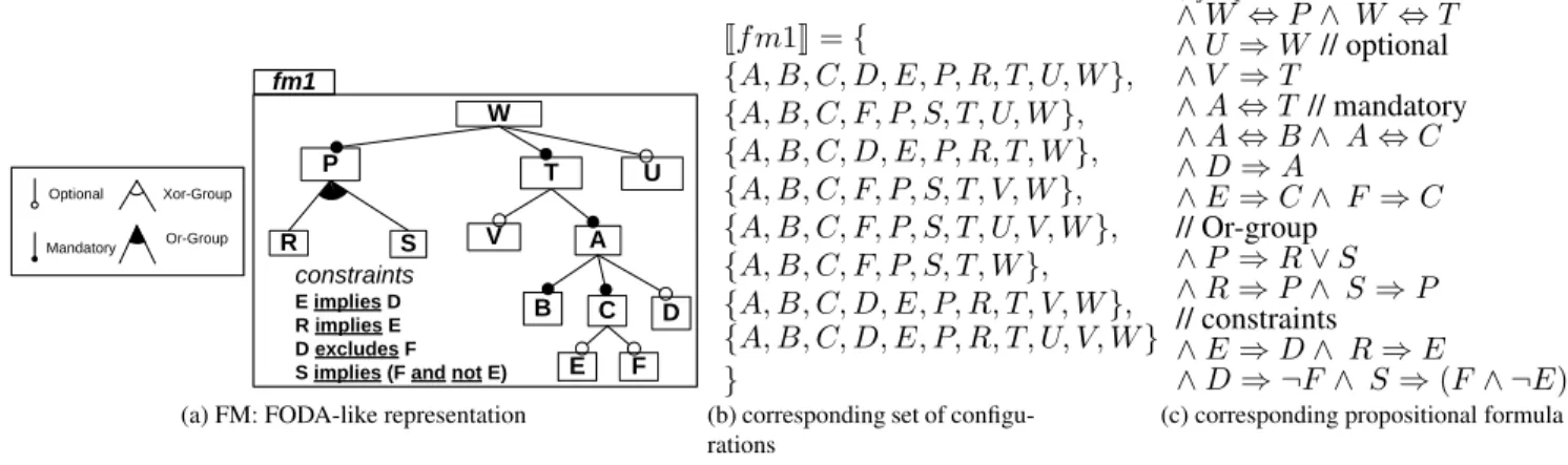
FMs were first introduced in the FODA method [19], which also provided a graphical representation through Feature Di-agrams. FMs are now widely adopted with support of formal semantics, reasoning techniques and tooling [8, 10, 12, 27]. An FM defines both a hierarchy, which structures features into levels of increasing detail, and some variability aspects expressed through several mechanisms. When decomposing a feature into subfeatures, the subfeatures may be optional or mandatory or may form Xor or Or-groups. In addition, any propositional constraints (e.g., implies or excludes) can be specified to express more complex dependencies between features. We consider that an FM is composed of a feature di-agram coupled with a set of constraints expressed in propo-sitional logic. Figure 1a shows an example of an FM. The feature diagram is depicted using a FODA-like graphical no-tation used throughout the paper.

The hierarchy of an FM is represented by a rooted tree G = (F , E, r) where F is a finite set of features and E ⊆ F × F is a finite set of edges (edges represent top-down hierarchical decomposition of features, i.e., parent-child relations between them) ; r ∈ F being the root feature.

An FM defines a set of valid feature configurations. A valid configuration is obtained by selecting features so that i) if a feature is selected, its parent is also selected; ii) if a parent is selected, all the mandatory subfeatures, exactly one subfeature in each of its Xor-groups, and at least one of its Or groups are selected; iii) propositional constraints hold. For example, in Figure 1a, {A, B, C, F, P, S, T, W} is a valid configuration, the features Dand Fcannot be selected at the same time and Ecannot be selected without Cdue to the parent-child relation between Eand C.

DEFINITION1 (Configuration Semantics). A configuration of an FM g is defined as a set of selected features. _JgK denotes the set of valid configurations of the FMg and is thus a set of sets of features.

FMs have been semantically related to propositional logic [12]. The set of configurations represented by an FM can be described by a propositional formula φ defined over a set of Boolean variables, where each variable corresponds to a feature (see Figure 1c for the formula corresponding to the FM of Figure 1a). The translation of FMs into logic rep-resentations allows one, as we will see in the next sections, to use reasoning techniques for automated FM analysis [10].

3.

Composition and Decomposition Support

In previous work [2, 4], we designed a set of composition and decomposition operators that produce a new FM from one or more than one input FMs. We have defined the se-mantics of these operators in terms of:

configuration semantics We consider that the primary mean-ing of an FM, known as its configuration semantics, is a set of legal configurations – sets of selected features that respect the dependencies entailed by the diagram and the cross-tree constraints. We thus define the semantics of each operator in terms of the relationship between the configuration sets of the input FMs and the resulting FM. feature hierarchy Another important property of an FM is the way features are organized – reflected in the feature hierarchy. We recall that two FMs can have identical con-figuration semantics, yet different hierarchies and thus ontological meaning [10, 29, 32]. As a result, we con-sider that the feature hierarchy should also be part of the semantics of the operators.

3.1 Aggregate

The aggregate operator supports cross-tree constraints be-tween features so that separated FMs can be inter-related. The input FMs are aggregated under a synthetic root syntheticf tso that the root features of input FMs are

child-mandatory features of syntheticf t. In addition, the

propo-sitional constraints are added in the resulting FM. For ex-ample, the aggregate operator can be used to compose four FMs together with constraints (see Figure 5, page 6).

The properties of the aggregated FM heavily depends on the set of propositional constraints used during the

aggre-W

constraints

E implies D R implies E D excludes F S implies (F and not E)

P R S fm1 A V T U B C D E F Optional Mandatory Xor-Group Or-Group

(a) FM: FODA-like representation

Jf m1K = { {A, B, C, D, E, P, R, T, U, W }, {A, B, C, F, P, S, T, U, W }, {A, B, C, D, E, P, R, T, W }, {A, B, C, F, P, S, T, V, W }, {A, B, C, F, P, S, T, U, V, W }, {A, B, C, F, P, S, T, W }, {A, B, C, D, E, P, R, T, V, W }, {A, B, C, D, E, P, R, T, U, V, W } }

(b) corresponding set of configu-rations φf m1 = W // root ∧ W ⇔ P ∧ W ⇔ T ∧ U ⇒ W // optional ∧ V ⇒ T ∧ A ⇔ T // mandatory ∧ A ⇔ B ∧ A ⇔ C ∧ D ⇒ A ∧ E ⇒ C ∧ F ⇒ C // Or-group ∧ P ⇒ R ∨ S ∧ R ⇒ P ∧ S ⇒ P // constraints ∧ E ⇒ D ∧ R ⇒ E ∧ D ⇒ ¬F ∧ S ⇒ (F ∧ ¬E)

(c) corresponding propositional formula

Figure 1. FM, set of configurations and propositional logic encoding gate. It may lead to situations where the aggregated FM does

not represent any valid configuration or includes dead or core features (see Definition 2). We consider that the aggregate operator is purely syntactical. As we will see, other comple-mentary techniques can be applied in case an SPL practi-tioner may want to simplify the aggregated FM or to reason about its properties.

3.2 Merge

The merge operator is dedicated to the composition of FMs that exhibit similar features (i.e., features with the same name). In this case, the merge operator can be used to merge the overlapping parts of the FMs and then to obtain an integrated FM. The merge uses name-based matching: two features match if and only if they have the same name. Configuration Semantics. The properties of a merged FM produced by an application of the merge operator are for-malized in terms of the sets of configurations of input FMs. Several modes are defined for the merge operator. We only describe here the modes that we will use in the remainder of the paper. The intersection mode is the most restrictive option: the merged FM, F Mr, expresses the common valid

configurations of F M1and F M2. The merge operator in the

intersection mode is denoted as follows: F M1⊕∩F M2 =

Result. The relationship between a merged FM Result in intersection mode and two input FMs F M1and F M2 can

be expressed as follows:

JF M1K ∩ JF M2K = JResultK

Another merge operator, called diff, is denoted as F M1⊕\

F M2 = Result. The following defines the semantics of

this operator:

JF M1K\JF M2K = {x ∈ JF M1K | x /∈JF M2K} = JResultK Hierarchy. Several FMs, with different hierarchies, can represent the same set of configurations [10, 29, 32]. So in particular several merged FMs can be produced and consis-tently represent the expected set of configurations while hav-ing different hierarchies. Intuitively, the more a parent-child relation occurs in the input FMs, the more an edge in the

merged hierarchy should be retained. The problem of choos-ing a hierarchy from amongst a set of hierarchies can be for-mulated as a minimum spanning tree problem (see details in [1]). An example of merge operation in intersection mode is given in Figure 8, page 7.

3.3 Slice Operator

The slice operator aims at simplifying or abstracting FMs by focusing on selected aspects of semantics. The overall idea behind FM slicing is similar to program slicing [36]. Program slicing techniques proceed in two steps: the subset of elements of interest (e.g., a set of variables of interest and a program location), called the slicing criterion, is first identified; then, a slice (e.g., a subset of the source code) is computed. In the context of FMs, we define the slicing criterion as a set of features considered to be pertinent by an SPL practitioner while the slice is a new FM.

A B C D E F constraints E implies D D implies E (a) [[fm2]] = {{A, B, C, D, E},{A, B, C, F}} W constraints E implies D R implies E P R S V A T U B C D E F (b) [[fmAll]] = [[fm1]]

Figure 2. Two slice operations on fm1 (see Figure 1a) Configuration Semantics. We define slicing as a unary operation on FM, denoted ΠFslice (F M ) where Fslice =

{f t1, f t2, ..., f tn} ⊆ F is a set of features.

The result of the slicing operation is a new FM, F Mslice,

such that:_{JF M}sliceK = {x ∩ Fslice| x ∈JF M K } (called the projected set of configurations).

Hierarchy. Intuitively, the hierarchy of F Mslice is such

that features are connected to their closest ancestor if their parent is not part of the slicing criterion. A formal definition can be found in [1]. Two examples of slice operation are given in Figure 2.

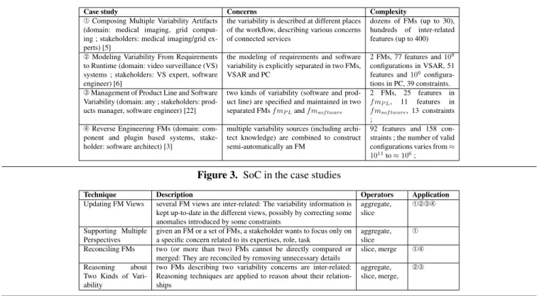
Case study Concerns Complexity À Composing Multiple Variability Artifacts

(domain: medical imaging, grid comput-ing ; stakeholders: medical imagcomput-ing/grid ex-perts) [5]

the variability is described at different places of the workflow, describing various concerns of connected services

dozens of FMs (up to 30), hundreds of inter-related features (up to 400) Á Modeling Variability From Requirements

to Runtime (domain: video surveillance (VS) systems ; stakeholders: VS expert, software engineer) [6]

the modeling of requirements and software variability is explicitly separated in two FMs, VSAR and PC

2 FMs, 77 features and 108

configurations in VSAR, 51 features and 106

configura-tions in PC, 39 constraints. Â Management of Product Line and Software

Variability (domain: any ; stakeholders: prod-ucts manager, software engineer) [22]

two kinds of variability (software and prod-uct line) are specified and maintained in two separated FMs f mP Land f msof tware

2 FMs, 25 features in f mP L, 11 features in

f msof tware, 13 constraints

; Ã Reverse Engineering FMs (domain:

com-ponent and plugin based systems, stake-holder: software architect) [3]

multiple variability sources (including archi-tect knowledge) are combined to construct semi-automatically an FM

92 features and 158 con-straints ; the number of valid configurations varies from ≈ 1011_{to ≈ 10}6_;

Figure 3. SoC in the case studies

Technique Description Operators Application

Updating FM Views several FM views are inter-related: The variability information is kept up-to-date in the different views, possibly by correcting some anomalies introduced by some constraints

aggregate, slice

ÀÁÂÃ

Supporting Multiple Perspectives

given an FM or a set of FMs, a stakeholder wants to focus only on a specific concern related to its expertises, role, task

aggregate, slice

À Reconciling FMs two (or more than two) FMs cannot be directly compared or

merged: They are reconciled by removing unnecessary details

slice, merge ÀÃ Reasoning about

Two Kinds of Vari-ability

two FMs describing two variability concerns are inter-related: Reasoning techniques are applied to reason about their relation-ships

aggregate, slice, merge,

ÁÂ

Figure 4. SoC in feature modeling

4.

Applying Separation of Concerns

Given these composition and decomposition mechanisms, we now argue that these operators, together with other rea-soning and editing operators, form a consistent and powerful support for SoC in feature modeling.

Several usage scenarios can be envisaged:

•When an FM is decomposed into smaller FMs (using the slice operator), one may need to reason about the differ-ent sets of configurations or simply modify the smaller FMs. The composition operators can be applied after-wards to recompose the smaller FMs ;

•When some FMs are composed with constraints (using the aggregate operator), one may need to simplify, re-decompose or check the satisfiability of the resulting composed FM ;

•Before merging two FMs, one may need to reconcile (or align) the two FMs in case the hierarchy and the vocabulary used in the two FMs differs ;

Beyond these simple examples, we now show that though the sole use of the composition / decomposition operators has practical interests, the area of applications grows when these operators are combined together1_.

The following sections will demonstrate either new capa-bilities in feature modeling or better scalability in represen-tative scenarios of the field. Each presented technique has been validated on experimental or real-world case studies. Figure 4 gives an overview of the contribution. It

charac-1_{The tooling and language support,FAMILIAR, is out of the scope of}

this paper. The interested reader can visit https://nyx.unice.fr/ projects/familiar/

terizes each technique, reports the operators involved in the realization of the technique as well as the practical use in case studies. The numbers correspond to the different case studies described in Figure 3, including the application do-main, the stakeholders involved, the concerns considered as well as the complexity of FMs.

4.1 Corrective Capabilities

Manual or automatic creation of FMs may generate anoma-liesin them. Generally, these anomalies are regarded as a negative property of an FM since it can easily decrease its maintainability or understandability.

DEFINITION2 (Dead and Core features). A feature f of an FM is dead if it cannot be part of any of the valid configura-tions. A featuref of an FM is a core feature if it is part of all valid configurations.

Error-free FMs. Benavides et al. identify different kinds of FM anomalies [10]: i) dead features (see Definition 2) ; ii)false optional features are core features (see Definition 2), despite not being modeled as mandatory ; iii) wrong feature group: For example, features may form an Or-group while being mutually exclusive (see features Rand Sin the FM of Figure 1a) ; iv) or redundancies [10] (e.g., cross-tree con-straints may be redundant). Despite the need of automatic support for anomaly analysis in FMs, there is a lack of pro-posals that focus on producing error-free FMs, i.e., FMs that do not contain anomalies as the ones mentioned above.

A form of corrective explanations has been developed in [10]. It indicates changes (or edits) to be made in the original FM so that it does not contain anomalies anymore.

These changes are suggestions, usually once anomalies have been detected and explained, to be applied to the original FM. In this case, the set of configurations of the original FM may be altered (e.g., a dead feature may no longer be dead once changes have been applied). This approach is more ap-propriate for handling human errors, for example, when an SPL practitioner elaborates an FM and unintentionally in-troduces errors. On the contrary automatic correction (or simplification)aims at removing anomalies from the origi-nal FM while the set of configurations remains exactly the same. Our contribution here takes place in this category, as automatic correction pursues a different objective: anoma-lies are not necessary errors but an intentional, controlled and/or temporary properties of an FM, for example, when automatic operations are conducted on FMs. As we will see in the next section, it usually happens when two (or more than two) FMs are inter-related by constraints. In this case, features may become dead or core features.

Automatic simplification using the slice. The slicing im-plementation we propose ensures, by construction, that there is no dead feature, correctly detects core features (thereby false optional features) and avoids redundancy in the repre-sentation (e.g., we add an implies/excludes constraint only if it is not already induced by the FM) [4]. Hence, we guarantee that the sliced FM does not contain anomalies. As a result, the slice operator can be used as an automated technique to correct anomalies of FMs while preserving the original set of configurations and hierarchy. Moreover, the corrective modifications applied to the original FM can be detected and reported to an SPL practitioner. For example, the slice oper-ation is performed on the FM of Figure 1a, f m1, using all features of f m1 as a slicing criterion. The resulting FM is f mAll (see Figure 2b). Obviously the set of configurations represented by f mAll is the same as the set of configura-tions represented by f m1, while their feature hierarchies are equal. We can notice that i) the features Rand Sform an Xor-group in f mAll (and no longer form an Or-group as in f m1) ; ii) the features Eand Fform an Xor-group (and are no longer optional as in f m1) ; iii) some constraints are no longer present in f mAll to avoid redundancy.

As an application, we directly used this correction tech-nique to automatically remove anomalies in the randomly generated FMs that served as inputs for our experimenta-tions (see Section 5.1 and 7). Both configuration sets and hierarchies were maintained while correcting anomalies. 4.2 Managing Different FM Views

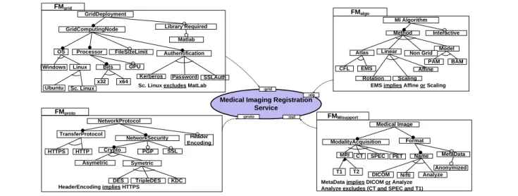
We illustrate the need to manage several FMs, possibly inter-related, using an example in the medical imaging domain. In this domain, medical imaging services (e.g., algorithms) are assembled to form complex processing chains (also called workflows). Variability affects different concerns or views of a medical imaging service. In Figure 5, the service is described through different views: information about the deployment on the grid, internal algorithms, the supported communication protocols and the type of handled medical

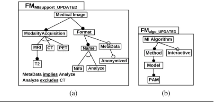
Format MetaData Anonymized Name Nifti Analyze ModalityAcquisition CT MRI T2 PET Medical Image FMMIsupport_UPDATED

MetaData implies Analyze Analyze excludes CT (a) FMalgo_UPDATED Interactive Model PAM MI Algorithm Method (b)

Figure 6. Updating FM views

images. As multiple sources of variation are present within a service, several FMs are used where each FM focuses on a specific view of a service. As shown in [5], these FMs can then be used to check consistency between composed services and to facilitate their coherent configurations. 4.2.1 Updating FM views

In practice, the different FM views of a service are not in-dependent. The workflow designer has to add constraints to enforce interactions between the FM views. In our example, we consider the following constraints:

M IServiceconstraints= {

(c1) F Mgrid.Kerberos ⇒ F Mproto.KDC (c2) F Mgrid.SSLAuth ⇔ F Mproto.SSL (c3) F MM Isupport.M RI ⇒ F Malgo.P AM (c4) F MM Isupport.CT ∨ F MM Isupport.SP EC

⇒ F Malgo.BAM

(c5) F MM Isupport.Anonymized

⇒ F Mproto.HeaderEncoding

(c6) ¬F Mgrid.GP U ∨ ¬F Malgo.Interactive (c7) F Malgo.Interactive ⇒ F Mgrid..Linux (c8) F MM Isupport.DICOM

⇒ F Mproto.Rotation ∧ F Mproto.P AM

(c9) F Malgo.Interactive ⇒ F Mproto.HeaderEncoding }

Determining the impact of these constraints on each FM view cannot be done manually or even automatically with current techniques and tools [10]. We rely on the corrective capabilities developed in Section 4.1 to perform the update of the different FM views.

Using the slice operator, it simply consists in i) aggre-gating the four feature models into a single one (fmService) with constraints mapped on it, ii) invoking slice four times producing as much sliced FMs, the slicing criterion being respectively the features of each of the four feature models. As a result, Figure 6a and Figure 6b correspond to the sliced FM with respectively the features of the FMs F MM Isupport

and F Malgo. The two other FMs are not impacted by the

constraints mapped on fmService.

4.2.2 Supporting multiple perspectives

On the same example, the slice operator can be used to extract other views (or perspectives) of a service. In Fig-ure 7, we captFig-ure expertises related to security featFig-ures or to the medical imaging domain. Two slice operations are applied and compute two FM views, stored into fmViewMI

Medical Imaging Registration Service :grid :proto :alg :out Sc. Linux excludes MatLab

FileSizeLimit Processor x32 x64 OS Windows Linux GridComputingNode GridDeployment Library Required GPU Bits Ubuntu Sc. Linux Authentification SSLAuth Password Kerberos Matlab FMgrid TransferProtocol HTTPS HTTP Header Encoding NetworkProtocol Crypto NetworkSecurity SSL PGP Asymetric Symetric DES TripleDES KDC FMproto HeaderEncoding implies HTTPS Format MetaData Anonymized Name

DICOM Nifti Analyze ModalityAcquisition CT SPEC MRI T1 T2 PET Medical Image FMMIsupport

MetaData implies DICOM or Analyze Analyze excludes (CT and SPEC and T1)

FMalgo Interactive Model PAM BAM Linear Rotation Affine Non Grid MI Algorithm Scaling Method Atlas CFL EMS

EMS implies Affine or Scaling

Figure 5. Variability and concerns within a medical imaging service and fmViewSecurity. The slicing criterion used to compute

fmViewMI(resp. fmViewSecurity) contains features from the FMs F MM I, F Malgoand F Mgrid(resp. F MM I, F Mproto

and F Mgrid). The slice guarantees that all the interactions

existing with other FM views are still enforced. 4.2.3 Practical applications

Reverse Engineering Architectural FMs.Besides the above application, the slicing technique was also extensively used in a tool-supported approach to reverse engineer software variability from an architectural perspective [3]. The pro-posed approach was evaluated when applied to FraSCAti, a large and highly configurable component and plugin-based system. Using the slicing technique an accurate view (i.e., an FM) of the software architecture was obtained. The idea was that the software architecture FM, originally produced by an extraction procedure, represents only an over approx-imation in terms of sets of valid configurations. Hence sev-eral sources of information were combined, namely software architecture, plugin dependencies and the correspondences between software elements and plugins. When combined through aggregation, slicing is used to update the view cor-responding to the software architecture part. The aggregated FM resulting from the combination of different variability sources and the bidirectional mapping contains 92 features

and 158 cross-tree constraints (CTCR2_{=84%). The slicing}

technique significantly reduced the over approximation of the original architectural FM (from ≈ 1011_{to ≈ 10}6_).

Variability in video surveillance.In the development of a video surveillance SPL, we represented the variability of the context and the variability of the software platform as two separated FMs [6]. 77 features and 108 configurations were present in the context FM while 51 features and 106

configurations were present in the software platform FM. The relationships between the two FMs were described as 39 rules (propositional constraints) relating features across models. Then, in line with specific requirements, we step-wise specialized the FM representing the context by remov-ing some features, by modifyremov-ing some feature groups, etc. After the specialization of the context FM, we needed to up-date the software platform FM. To do so, we aggregated the specialized context FM and the software platform FM to-gether with rules. We used the slice operator on the aggre-gated FM by only including the set of features related to the software platform. We observed that from a specification of a context, the possible configurations in the software plat-form can be highly reduced. We applied the techniques on different scenarios: the average number of features to

con-2_{CTCR is the ratio of the number of features in the constraints to the}

number of features in the feature hierarchy.

GPU MIService Library Required Matlab Analyze excludes CT Interactive Model PAM MI Algorithm Method Format Name Nifti Analyze ModalityAcquisition CT MRI T2 PET Medical Image fmViewMI

(a) Medical Image expert view

TransferProtocol HTTPS HTTP Header Encoding NetworkProtocol Crypto NetworkSecurity SSL PGP Asymetric Symetric DES TripleDES KDC

Anonymized implies HeaderEncoding HeaderEncoding implies HTTPS SSL ó SSLAuth Kerberos implies KDC MetaData Anonymized MIService Authentification SSLAuth Password Kerberos fmViewSecurity

(b) Security expert view

sider in the software platform FM was less than 104(instead of 106_{configurations).}

4.3 Reconciling Feature Models

When managing a set of FMs, the different stakeholders in-volved in the SPL development may have to put together very similar variability information but with a different structure. For example, in the medical imaging domain, dif-ferent suppliers (scientists, research teams, companies, etc.) provide imaging services and may use different hierarchies, concepts, vocabulary, etc. when elaborating the FMs. 4.3.1 Technique and example

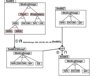
Let us consider two FMs, f mM I1 and f mM I2, in Fig-ure 8. The two FMs differ. In particular, featFig-ures Open, Pro-prietary, NiftiI, NiftiII are present in f mM I1 but not in f mM I2. Intuitively, more structure and details are mod-eled in f mM I1. As a result, a comparison (see Defini-tion 3) or a merging (see SecDefini-tion 3.2) of the two FMs leads to counter intuitive results, i.e., the intersection of the two configuration sets is empty (see line4and5of theFAMILIAR

script below). Looking at the two FMs, some configurations seem to correspond, for example, the valid configuration

{M edicalImage, DICOM }of f mM I2 with the

configura-tion{M edicalImage, Open, DICOM }of f mM I1. We thus

need to reconcile (or align) the two FMs and allow an SPL practitioner to align in a coherent way information from f mM I1 and f mM I2.

DEFINITION3 (Kind of edits and Comparison). Let f and g be two FMs. f is a specialization of g if _{Jf K} ⊂ _{JgK. f is} a generalization of g if JgK ⊂ Jf K. f is a refactoring of g if JgK = Jf K. f is an arbitrary edit of g if f is neither a specialization, a generalization nor a refactoring of g. A comparison computes the relationship between two FMs.

fmMI1

fmMI2

MedicalImage

Nifti DICOM SPI

fmMI3

MedicalImage

Nifti DICOM SPI

∩ Π MedicalImage, Nifti, DICOM, SPI, GE (fmMI1) fmMI1Sliced

MedicalImage

Nifti DICOM SPI GE 1

2 MedicalImage

Open Proprietary

Nifti DICOM SPI GE

NiftiI NiftiII

Figure 8. Slicing (À) to reconcile FMs and allow, e.g., comparison or merging (_Á)

Using the slice operator, we simply remove features of f mM I1 i) that structure the feature model (i.e., features

Open, Proprietary) and ii) that can be abstracted by a single

feature (i.e., Niftiabstracts features NiftiIand NiftiII). Then, the comparison can be computed or the merge operator can be used as in Figure 8.

4.3.2 Practical application

Besides the medical imaging domain, we also used the tech-niques described above for the reverse engineering of FraS-CAti architectural FM. The architectural FM resulting from the automatic extraction (see Section 4.2.3) was compared with another architectural FM, this time manually designed by the software architect (SA) of FraSCAti. Unfortunately, the direct comparison yields to unexploitable results, mainly due to the difference of granularity (i.e., some features in one FM are not present in the other). Basic manual edits of FMs were unpractical as we needed to safely remove fea-tures involved in several constraints or that were in the mid-dle of the hierarchy. The slicing operator was extensively ap-plied to remove unnecessary details in both FMs. Once the FMs have been reconciled, the two FMs can be compared so that the differences between them can be identified. This encourages the SA to correct his initial model [3].

4.4 Reasoning about Two Kinds of Variability

In SPL engineering, two kinds of variability are usually dis-tinguished [22, 23]: software (or internal) variability, hidden from customers, as opposed to product line (PL) (or exter-nal) variability, visible to them. Software variability and PL variability can be seen as two concerns of an SPL. Metzger et al. proposed a formal and concise approach for separat-ingPL variability and software variability and enabling au-tomatic analysis [22]. The two concerns are modeled as two FMs and inter-related by constraints. The authors mention several properties that should be checked when reasoning about the two kinds of variability. We now revisit here the approach defended in [22] and show how the operators can be combined to support SoC in this context.

4.4.1 Realized-by property

An important property of an SPL is realizability, i.e., whether the set of products that the PL management decides to of-fer is fully covered by the set of products that the software platform allows building. In Figure 9, we want to ensure that for each valid selection/deselection of features of f mP L

per-formed by a customer, there exists at least one corresponding software product described by f msof tware. The PL

vari-ability is documented using f mP L, the software variability

is documented using another FM (see f msof tware) and the

two FMs are related through constraints (see mapSof tP L).

Note that the mapping between features of f mP L and

f msof tware is not necessarily one-to-one. To this end we

first reason about the relationship between f msof twareand

f mP L. We compute f mG, the aggregation of f mP L and

f msof twareand add the constraints mapSof tP L.

In terms of FMs, the realizability property can be for-mally expressed (FP Lthe set of features of f mP L):

Online Store Debit Card Payment Payment Upon Voice fmSoftware Check of Credit History Credit Card Payment Online Store Debit Card Payment Payment Upon Voice fmPL Check of Credit History V2 => V3 V1 ó f1 V2 ó f2 V3 ó f3 f2 f1 V1 V2 V3 f3 f4 r VP1

Figure 9. Software and PL Variability (adapted from [22]) Intuitively, if the restriction of the PL features toJf mGK is equivalent to the original_{Jf m}P LK, the constraints mapSof tP L has no effect on the PL part of f mGand thus the realizability

property holds. Otherwise some products cannot be realized in the platform. Equation 1 implies to check if f mP L is a

refactoring (see Definition 3) of ΠFP L(f mG). Using the

ag-gregate, slice and merge diff operators, we can automatically check this property. First, we slice the aggregated FM f mG

by only including FP L, the set of features of f mP L. The

slice produces a new FM, denoted f mP LP rime. Formally:

f mP LP rime = ΠFP L(f mG)

Then, we compare the resulting FM, f mP LP rime, with

the original PL model, f mP L. If f mP LP rime is not a

refactoring of f mP L, the realizability property is

vio-lated since some existing products of f mP L are removed

in f mP LP rime and no product is added. Finally, we can

compute the set of products that are in f mP L but not in

f mP LP rime using the merge operator in diff mode. The

merge operator produces f mP LDif f.

Back to the example of Figure 9, we obtain that the realizability property does not hold and that three products proposed to customers cannot be realized by the platform:

Jf mP L⊕\f mP LP rimeK = Jf mP LDif fK = {{V 1, V 3, V 2, V P 1}, {V 1, V P 1}, {V 3, V P 1}}

Only the following two products can be realized:

Jf mP L⊕∩f mP LP rimeK = Jf mP LInterK = {{V 1, V 3, V P 1}, {V 2, V 3, V P 1}}

4.4.2 Non useful products

A product is useful if it is a possible realization of a PL mem-ber. As argued in [22], the list of non-useful products is a symptom of unused flexibility of the software platform. It can be on purpose, for example, justified by future market-ing extensions. The usefulness property can be seen as the "symmetric" of the realized-by property. Formally, all prod-ucts are useful if the following relation holds:

∀cp ∈_{Jf m}sof twareK, cp ∈ JΠFsof tware(f mG)K Hence, similar techniques involving aggregate, slice and merge can be used to check the property.

4.4.3 Practical applications

Reasoning about two concerns.We apply the techniques us-ing the larger example described in [22]. We successfully retrieved the same results, but our approach is more efficient since we do not enumerate configurations/products as they do. Moreover, high-level operators (slice, aggregate, com-pare, merge) facilitate the reasoning realization and offer a systematic solution for SPL practitioners when understand-ing and maintainunderstand-ing the two FMs. It should be noted that the technique for updating views (see Section 6) can be applied in such contexts, for example, to remove dead features in the PL or software model.

Reasoning about variability properties. In the develop-ment of video surveillance systems, a key issue is to ensure that, given a valid configuration of the context, a software configuration can always be obtained. This property is simi-lar to the realized-by property and can be checked using the same techniques. We successfully scale for this case study, whereas it was clearly not the case with the enumerative technique proposed in [22].

5.

Towards Scalable Technique to Separate

Concerns

Central to the support for SoC in feature modeling is the ability to decompose (i.e., slice) FMs. All applications de-scribed in the previous section make extensive use of the slicing technique. It is thus crucial to provide a scalable im-plementation of the slice operator. A syntactical technique is not adequate, especially in the presence of cross-tree con-straints. A technique based on the enumeration of configu-rations is not scalable, since the number of configuconfigu-rations is exponential to the number of features. To avoid these lim-itations, we developed a dedicated technique that consists in first computing the propositional formula representing the projected (see Section 3.3) set of configurations. The compu-tation of the propositional formula is essential for reasoning about the projected set of configurations but also for synthe-sizingthe FM. As detailed in [4], propositional logic tech-niques [12, 29] can be applied to construct an FM (includ-ing its hierarchy, variability information and cross-tree con-straints) from the formula. In this section, we focus on the computation of the propositional formula. We report on the practical limits of an implementation based on binary deci-sion diagrams (BDDs). We describe a symbolic technique that outperforms a BDD-based implementation and that can efficiently decompose FMs with thousands of features. Propositional Formula Encoding. First, we describe the encoding of the projected set of configurations as proposi-tional formula For a slicing F Mslice= Πf t1,f t2,...,f tn(F M ),

the propositional formula φslice corresponding to F Mslice

can be defined as follows:

φslice≡ ∃ f tx1, f tx2, . . . f txm0 φ

where f tx1, f tx2, . . . f txm0 ∈ (F \ F_slice) = F_removed.

Intuitively, all occurrences of features that are not present in any configuration of F Msliceare removed by existential

quantification in φ. φsliceis obtained from φ by existentially

quantifying outvariables in Fremoved.

DEFINITION4 (Existential Quantification). Let v be a Boolean variable occurring inφ. φ|v (resp.φ|¯v) isφ where variable

v is assigned the value True (resp. False). Existential quan-tification is then defined as∃v φ =def φ|v∨ φ|¯v.

5.1 BDD-based Implementation

In previous work [4], we rely on BDDs [11] to compute the propositional formula. A BDD is a compact representation of a Boolean function (e.g., a propositional formula). BDDs can be efficiently used to compute the propositional formula described above since computing the existential quantifica-tion can be performed in at most polynomial time with re-spect to the sizes of the BDDs involved [11]. Furthermore, BDDs can be used to synthesize an FM in polynomial time regarding the size of the BDD representing the input propo-sitional formula [12]. A major drawback of BDDs is that finding an optimal variable ordering during BDD construc-tion is NP-hard [11]. Some heuristics have been developed and successfully compile FMs to BDDs for a number of fea-tures up to 2000 [20].

The goal of our experiment was to determine the scal-ability of the BDD-based implementation w.r.t. the size of the input FMs (i.e., number of features) and the size of the slicing criterion (i.e., number of features to include). For the experiment, we reuse the heuristics (i.e., Pre-CL-MinSpan) developed in [20] to reduce the size of BDDs. For a first evaluation, we used several small and medium-sized FMs that were publicly available from SPLOT [21] repository as well as FMs from our case studies. We performed our ex-periments on more than 100 FMs, the bigger one having 290 features. We found that computing the slice is almost instantaneous in all cases. To go further, we randomly gen-erated FMs with several hundreds of features. We varied i) the number of features, noted #f eatures, from 100 to 2000 features (the known practical limits of BDD) ; ii) CT CR from 10% to 100%. We used the publicly available proce-dure described in [21] to randomly generate the FMs. In each generated model, each type of mandatory, optional, Xor and Or-groups was added with equal probability. For each FM, we randomly generated a slicing criterion. We varied the percentage of features to slice between 100% (no existen-tial quantification is performed) and 1% (almost all features are existentially quantified). The main results show that:

•The synthesis of the feature diagram has practical lim-its (up to 800 features3). This limit also applies in our context. We observed that the slicing technique can scale even for an FM with 2000 features if the percentage of features to slice is ≤ 35%. The reason is that the size of a BDD will always be smaller or at least unchanged after existential quantification ;

3_{Janota et al. reported that the BDD-based algorithm proposed in [12]}

scales up only for FMs with 300/400 features [18], but did not use the heuristics proposed in [20]

•The primary limit of the BDD-based implementation lies in the difficulties to construct BDD from the original FM. In particular, the total number of features in the input FM should not be more than 2000 features, otherwise it is impossible to having a BDD-representation of the formula. It should be noted that whenever an FM can be represented as a BDD, φslice can be computed. Hence

the encoding of φslicecan scale up to 2000 features with

a CTCR of 10, whatever the slicing criterion is ; 5.2 SAT-based Implementation

She et al. proposed techniques to reverse engineer very large FMs (i.e., with more than 5000 features) [29]. As shown above BDDs do not scale for this order of complexity and therefore the slicing operator cannot process such FMs. She et al. adapted their previous techniques and now rely on satisfiability (SAT) solvers (rather than BDDs as in [12]). They reported that the use of SAT solvers is significantly more scalable. Hence a SAT-based implementation of slicing is an interesting perspective that motivates our work.

We identify two main issues. First, the size of the for-mula exponentially increases when existential quantification is performed many times, i.e., the number of clauses dou-bles at each iteration. It may become an issue when the size of Fremovedis important, even for small FMs. Second, SAT

solvers require a formula to be in conjunctive normal form (CNF). It is straightforward to translate the propositional for-mula of an FM into CNF. However, when existential quan-tification is performed, the resulting formula is not in CNF (see Definition 4). To tackle the first issue, we substitue each feature of Fremoved only in those clauses that contain the

feature. More formally, let f t be a feature of Fremoved, φ a

formula in CNF decomposed as follows:

φ = p(f t, φ) ∧ c(f t, φ) where c(f t, φ) denotes the conjunction of the clauses that do not contain the feature f t and p(f t, φ) denotes the conjunction of the clauses that do contain the feature f t. The existential quantification of f t in φ produces a new formula φ0_{defined as follows:}

φ0 = φ|f t∨ φ|f t¯ = (p(f t, φ)|f t∨ p(f t, φ)f t¯) ∧ c(f t, φ)

Example. We consider f m1 of Figure 1a (see page 3). We slice f m1 using as slicing criterion all features except

Tand V(i.e., Fremoved = {T, V }). It should be noted that

the existential quantification of Tand Vcan performed in any order. In this example, we first perform the existential quantification of T, producing the following propositional formula: φ0_{f m}

1 = ((W ⇔ T rue ∧ V ⇒ T rue ∧ A ⇔

T rue) ∨ (W ⇔ F alse ∧ V ⇒ F alse ∧ A ⇔ F alse)) ∧ c(V, φ) ∧ T rue ∧ ¬F alse.

Then we iterate by performing the existential quantifica-tion of Vin φ0_{f m}

1. We can observe that at each iteration the

formula can be symbolically simplified in many ways. For instance, Tcannot be evaluated to False in φ0_{f m1} and there-fore the disjunctive clause can be removed. We can also ob-serve that A ⇔ T rue ≡ T rue but we do not consider this kind of simplification since features included in the slicing criterion, likeA, must not be removed. However we can

sim-plify φ0_{f m1}considering that V ⇒ T rue ≡ T rue since Vis included in the slicing criterion. An additional optimisation, related to symbolic simplification, is the order in which the features are existentially quantified. Indeed, we observe that some features are likely to be simplified. We use an heuristic that existentially quantifies in priority features that are at the bottom of the feature hierarchy. To tackle the second issue, we transform the resulting propositional formula into CNF at each iteration (i.e., for each existential quantification of a feature f t). It should be noted that we only need to consider the transformation of (p(f t, φ)|f t ∨ p(f t, φ)f t¯) into CNF

since c(f t, φ) is already in CNF.

Generated FMs.For the evaluation of the technique, we used the same FMs as with the experiments conducted for the BDD-based implementation. We also generated FMs with 2000 ≥ #f eatures ≥ 10000 with the same param-eters as previously described (10000 features is the prac-tical limit admitted in the literature [10, 21, 32]). We first verified that the techniques described above are necessary since a naive substitution strategy that does not compute c(f t, φ) is not scalable (scalability issues are observed for #f eatures ≥ 50). Using our technique, we found that: i) computing the propositional formula is almost instanta-neous for all FMs of SPLOT (less than one second, what-ever the size of the slicing criterion is); ii) the SAT-based implementation scales for #f eatures ≤ 10000 whatever the size of the slicing criterion is; iii) the order in which the features are existentially quantified is of prior impor-tance: we begin to observe scalability issues when quan-tifying first the features that are in top of the feature hi-erarchy for #f eatures ≥ 2000 ; iv) for very large FMs (#f eatures ≥ 5000), the computation time is inadequate for an interactive use of the slice operator (up to 20 minutes). Real world FMs. As stated early, automated extraction techniques now produce very large FMs from existing soft-ware systems. We applied our technique to three inde-pendent systems relating to the operating system domain (Linux, eCos, and FreeBSD). Linux and eCos have FMs whereas FreeBSD has not. She et al. reverse engineer the propositional formula of FreeBSD and develop techniques to interactively specify the hierarchy [29]. For the experi-ment, we directly applied the slicing technique on the for-mula of FreeBSD. It should be noted that, in this specific case, we cannot use the heuristic mentioned above since we do not have access to the hierarchy of FreeBSD. We ran-domly generated the order in which features are existentially quantified. The technique succeeded almost instantaneously (FreeBSD has 1203 features). We also succeeded on eCos that has over 1200 features.

Finally, we applied our technique to the FM of Linux which exhibits 6300 features. Contrary to the results ob-tained from the two other operating systems or from the experimental study described above, we scaled only for less than 60% of features included in the slicing criterion (whereas this percentage drops to 1% in the other cases). In order to understand the reasons of this limitation, we need to

compare the experimental conditions of the generated FMs with the properties of the Linux FM. The Linux model con-tains very small percentages of mandatory features (5%), grouped features (3%) – Linux features are mostly op-tional (92%). whereas in each generated model, each type of mandatory, optional, Xor and Or-groups was added with equal probability (25%). We can make the assumption that the slice operator is dependent on certain shapes of FMs, and/or certain kinds of constraints. We need to understand the impact of FM properties regarding the scalability of the slice operator. As future work, we plan to characterize more precisely the lack of scalability w.r.t. the Linux FM and de-velop new heuristics or specific techniques.

6.

Comparison with Other Solutions

We now review existing approaches that have been devel-oped to support SoC in FMs. We point out their relations to the SoC techniques that have been identified (see Fig-ure 4) and illustrated by different case studies in Section 4. To this end, we rely on the numbers used in Figure 3, each corresponding to a case study. The general conclusion is that without the new capabilities brought by our solution (i.e., the combined use of composition and decomposition operators), some analysis and reasoning operations would not be made possible in the different case studies.

Composition. A few works consider some forms of com-position for FMs and suggest the use of a merge opera-tor [7, 15, 27, 28]. An in-depth comparison of implemen-tation approaches is performed in [2]. Our proposal goes further since we clarified the semantics of the merge and showed that the merge alone is not sufficient to realize com-plex management tasks in the case studies _{À and Â. It} rather has to be combined with decomposition and reason-ing mechanisms. Several approaches use several and inter-related FMs and views [15, 19, 22, 24, 35]. As shown, the aggregate operator combined with the slice can be used in such contexts to update the different views, to support multi-ple perspectives or to reason about properties of the FMs (see case studies_{À, Á, Â and Ã). In [26], the authors tackled the} problem of mapping problem-space features into solution-space features and proposed to use default logic. Our con-tributions rely on propositional logics and therefore are not applicable to this work. Thompson et al. proposed to specify a product family from n perspectives: one family-hierarchy per view such as software or hardware [31]. It is a form of SoC that is particularly needed in the case studies_{À or Á. A} set-theoretic foundation is proposed: it can be expressed and realized using FMs and the presented techniques.

Decomposition. Thüm et al. [32] presented an automated and scalable technique to characterize the kinds of edit be-tween two FMs. An original property of the technique is that they distinguish abstract features from concrete features when reasoning. Abstract features are, in their work, non-leaf features. We consider this is the role of an SPL prac-titioner to explicitly determine which features are abstract

(as shown in the example of Section 4.3, abstract features are not necessary non-leaf features). Our technique is thus more general and realize the vision of [27] that makes the distinction between features that are of interest per se (i.e., that will influence the final product) and others. As we have shown, reasoning about the relationship of two FMs (and thus using the comparison operator developed in [32]) is inappropriate until FMs are not reconciled (see case stud-ies _{À and Ã). From our experience, tool supported} tech-niques, such as the safe removal of a feature by slicing, are not desirable but mandatory (i.e., basic manual edits of FMs are not sufficient) in this context. Recently, Thüm et al. [33] extend the work described in [32] and propose to make abstract features explicit in FMs. They show how a propositional formula can be retrieved describing the set of distinct "program variants", corresponding to combination of concrete features. Interestingly, Thüm et al. plan to ap-ply their techniques to SPL testing. We see this work as an application of the slicing technique where all features but abstract features are part of the slicing criterion. Our technique for computing the propositional formula is sim-ilar to the technique described in [33]. In addition we de-veloped an heuristic that determines the order in which the features are existentially quantified. We also applied to very large FMs and reported scalability results. In the context of feature-based configuration, techniques have been proposed to separate the configuration process in different steps or stages [13]. Our work is complementary since we propose techniques to decompose FMs. Hubaux et al. provide view mechanisms to decompose a large FM [17]. However they do not propose a comprehensive solution when dealing with cross-tree constraints. Furthermore we have shown that the decomposition of FMs has several other interesting applica-tions beyond the support of multiple perspectives (see case studies_{À, Á, Â and Ã). Benavides et al. survey the} liter-ature of automated reasoning about FMs [10]. To the best of our knowledge, there is no existing work for correcting anomalies in FMs. Furthermore, existing approaches men-tioned in [10] and discussed above either focus on composi-tion or decomposicomposi-tion, but they do not try to combine the two mechanisms for supporting SoC in feature modeling. The "tyranny of the dominant decomposition” is a general issue for aspect-oriented approaches [30]. In [9], Batory et al. introduced multi-dimensional SoC where a dimension is a set of features addressing a particular concern. We can see a dimension as a slicing criterion. The approach of Batory et al. does not generate views but rather composes features along each dimension. It is thus complementary and can be used to produce parts of a system, being services (case study À), components (case study Á) or plugins (case study Ã). Rosenmüller et al. develop compositional support to manage different FMs, each focusing on a specific dimension [25]. They do not consider composition of FMs that introduce anomalies and do not propose automated decomposition (as needed in all case studies).

7.

Threats to Validity

Threats to external validity are conditions that limit our abil-ity to generalize the results of our operators and experiment to industrial practice. Our first concern is whether generated FMs or Linux FM used in the experiments (see Section 5) are representative of industrial usage. Our second concern is whether the composition and decomposition operators are expressive and intuitive enough to support activities of SPL practitioners. As summarized by Figure 4 and Figure 3, the operators have been applied to different domains for differ-ent purposes and by differdiffer-ent people (external to our team). Moreover we identify several works in the literature that can benefit from the techniques (see Section 6).

A first internal threat concerns the correctness of the oper-ators implementation. In particular, the slice operator is sup-posed to guarantee that some semantic properties are pre-served. Our implementation is currently checked by a com-prehensive set of unit tests, complemented by cross-checked testing with other operations. For instance, we compared the formulas produced by the BDD-based and SAT-based im-plementation of the slice operator. We also manually veri-fied a large number of slice examples. Besides we observed that randomly generated FMs may contain a lot of anoma-lies (e.g., dead features or wrong feature group). We used this opportunity to gain further confidence in our implemen-tation and applied our slicing technique to automatically cor-rect anomalies in generated FMs (see Section 4.1). We au-tomatically checked that the original FM and the slice (i.e., corrected) FM were equivalent in terms of sets of configu-rations, that the slice FM did not contain any anomaly, and that the hierarchy conforms to the original FM.

8.

Conclusion

In this paper, we described how a set of complementary op-erators (aggregate, merge, slice) can be used to provide a powerful support for SoC in feature modeling. We showed how the operators can assist in tedious and error prone tasks such as automated correction of FM anomalies, update and extraction of FM views, reconciliation of FMs or reasoning about properties of FMs. The operators bring new capabil-ities to the FM users for supporting SoC in feature model-ing and when we revisited and reimplemented existmodel-ing ap-proaches with them, we observed a better scalability. Both these new capabilities and scalability results enabled us to apply SoC in feature modeling to different domains (medi-cal imaging, video surveillance) and for different purposes (scientific workflow design, variability modeling of context and software platform, reverse engineering). We also devel-oped a technique to implement the slice operator that scales up to FMs with 10000 features in certain conditions. As fu-ture work, we plan to study practical usage and applicability of the proposed techniques.

Acknowledgments. Dr. Acher’s work is supported by the IAP Programme, the Belgian Science Policy under the MoVES project, the FNRS, and an FSR grant, co-funded by Marie-Curie actions of the European Commission.

References

[1] M. Acher. Managing Multiple Feature Models: Foundations, Language and Applications. PhD thesis, 2011.

[2] M. Acher, P. Collet, P. Lahire, and R. France. Compar-ing approaches to implement feature model composition. In ECMFA’10, volume 6138 of LNCS, pages 3–19, 2010. [3] M. Acher, A. Cleve, P. Collet, P. Merle, L. Duchien, and

P. Lahire. Reverse engineering architectural feature models. In ECSA’11, volume 6903 of LNCS, pages 220–235, 2011. [4] M. Acher, P. Collet, P. Lahire, and R. France. Slicing feature

models. In ASE’11, pages 424–427. IEEE, 2011.

[5] M. Acher, P. Collet, P. Lahire, A. Gaignard, R. France, and J. Montagnat. Composing multiple variability artifacts to as-semble coherent workflows. Software Quality Journal (Spe-cial issue on Quality Engineering for SPLs), 2011.

[6] M. Acher, P. Collet, P. Lahire, S. Moisan, and J.-P. Rigault. Modeling variability from requirements to runtime. In ICECCS’11, pages 77–86. IEEE, 2011.

[7] V. Alves, R. Gheyi, T. Massoni, U. Kulesza, P. Borba, and C. Lucena. Refactoring product lines. In GPCE’06, pages 201–210. ACM, 2006.

[8] S. Apel and C. Kästner. An overview of feature-oriented software development. Journal of Object Technology (JOT), 8(5):49–84, July/August 2009.

[9] D. Batory, J. Liu, and J. N. Sarvela. Refinements and multi-dimensional separation of concerns. SIGSOFT Softw. Eng. Notes, 28:48–57, 2003.

[10] D. Benavides, S. Segura, and A. Ruiz-Cortes. Automated analysis of feature models 20 years later: a literature review. Information Systems, 35(6), 2010.

[11] K. S. Brace, R. L. Rudell, and R. E. Bryant. Efficient imple-mentation of a bdd package. In DAC ’90: Design Automation Conference, pages 40–45. ACM, 1990.

[12] K. Czarnecki and A. Wasowski. Feature diagrams and logics: There and back again. In SPLC’07, pages 23–34. IEEE, 2007. [13] K. Czarnecki, S. Helsen, and U. Eisenecker. Staged config-uration through specialization and multilevel configconfig-uration of feature models. Software Process: Improvement and Practice, 10(2):143–169, 2005.

[14] D. Dhungana, P. Grünbacher, R. Rabiser, and T. Neumayer. Structuring the modeling space and supporting evolution in software product line engineering. Journal of Systems and Software, 83(7):1108–1122, 2010.

[15] H. Hartmann and T. Trew. Using feature diagrams with con-text variability to model multiple product lines for software supply chains. In SPLC’08, pages 12–21. IEEE, 2008. [16] H. Hartmann, T. Trew, and A. Matsinger. Supplier

indepen-dent feature modelling. In SPLC’09, pages 191–200. IEEE, 2009.

[17] A. Hubaux, P. Heymans, P.-Y. Schobbens, D. Deridder, and E. Abbasi. Supporting multiple perspectives in feature-based configuration. Software and Systems Modeling, pages 1–23. [18] M. Janota, V. Kuzina, and A. Wasowski. Model construction

with external constraints: An interactive journey from seman-tics to syntax. In MODELS’08, volume 5301 of LNCS, pages 431–445, 2008.

[19] K. Kang, S. Kim, J. Lee, K. Kim, E. Shin, and M. Huh. Form: A feature-oriented reuse method with domain-specific reference architectures. Annals of Software Engineering, 5(1): 143–168, 1998.

[20] M. Mendonca, A. Wasowski, K. Czarnecki, and D. Cowan. Efficient compilation techniques for large scale feature mod-els. In GPCE’08, pages 13–22. ACM, 2008.

[21] M. Mendonca, A. W ˛asowski, and K. Czarnecki. SAT-based analysis of feature models is easy. In SPLC’09, pages 231– 240. IEEE, 2009.

[22] A. Metzger, K. Pohl, P. Heymans, P.-Y. Schobbens, and G. Saval. Disambiguating the documentation of variability in software product lines: A separation of concerns, formaliza-tion and automated analysis. In RE’07, pages 243–253, 2007. [23] K. Pohl, G. Böckle, and F. J. van der Linden. Software Product Line Engineering: Foundations, Principles and Techniques. Springer-Verlag, 2005. ISBN 3540243720.

[24] M.-O. Reiser and M. Weber. Multi-level feature trees: A prag-matic approach to managing highly complex product families. Requir. Eng., 12(2):57–75, 2007.

[25] M. Rosenmüller, N. Siegmund, T. Thüm, and G. Saake. Multi-dimensional variability modeling. In VaMoS’11, pages 11–20. ACM, 2011.

[26] F. Sanen, E. Truyen, and W. Joosen. Mapping problem-space to solution-space features: a feature interaction approach. In GPCE ’09, pages 167–176. ACM, 2009.

[27] P.-Y. Schobbens, P. Heymans, J.-C. Trigaux, and Y. Bontemps. Generic semantics of feature diagrams. Comput. Netw., 51(2): 456–479, 2007.

[28] S. Segura, D. Benavides, A. Ruiz-Cortés, and P. Trinidad. Au-tomated merging of feature models using graph transforma-tions. In GTTSE ’07, volume 5235 of LNCS, pages 489–505, 2008.

[29] S. She, R. Lotufo, T. Berger, A. Wasowski, and K. Czarnecki. Reverse engineering feature models. In ICSE’11, pages 461– 470. ACM, 2011.

[30] P. Tarr, H. Ossher, W. Harrison, and S. M. Sutton, Jr. N degrees of separation: multi-dimensional separation of concerns. In ICSE’99, pages 107–119. ACM, 1999.

[31] J. M. Thompson and M. P. E. Heimdahl. Structuring product family requirements for n-dimensional and hierarchical prod-uct lines. Requirements Engineering, 8(1):42–54, 2003. [32] T. Thüm, D. Batory, and C. Kästner. Reasoning about edits to

feature models. In ICSE’09, pages 254–264. ACM, 2009. [33] T. Thüm, C. Kästner, S. Erdweg, and N. Siegmund. Abstract

features in feature modeling. In SPLC’11, pages 191–200. IEEE, Aug. 2011.

[34] T. T. Tun and P. Heymans. Concerns and their separation in feature diagram languages - an informal survey. In Interna-tional workshop SCALE@SPLC’09, pages 107–110, 2009. [35] T. T. Tun, Q. Boucher, A. Classen, A. Hubaux, and P.

Hey-mans. Relating requirements and feature configurations: A systematic approach. In SPLC’09, pages 201–210. IEEE, 2009.

[36] M. Weiser. Program slicing. In ICSE ’81, pages 439–449. IEEE, 1981.