HAL Id: hal-01167185
https://hal.inria.fr/hal-01167185
Submitted on 24 Jun 2015
HAL is a multi-disciplinary open access
archive for the deposit and dissemination of
sci-entific research documents, whether they are
pub-lished or not. The documents may come from
teaching and research institutions in France or
abroad, or from public or private research centers.
L’archive ouverte pluridisciplinaire HAL, est
destinée au dépôt et à la diffusion de documents
scientifiques de niveau recherche, publiés ou non,
émanant des établissements d’enseignement et de
recherche français ou étrangers, des laboratoires
publics ou privés.
Compiling High Performance Recursive Filters
Gaurav Chaurasia, Jonathan Ragan-Kelley, Sylvain Paris, George Drettakis,
Fredo Durand
To cite this version:
Gaurav Chaurasia, Jonathan Ragan-Kelley, Sylvain Paris, George Drettakis, Fredo Durand.
Com-piling High Performance Recursive Filters. High Performance Graphics, Eurographics/ACM
SIG-GRAPH, Aug 2015, Los Angeles, United States. �hal-01167185�
Compiling High Performance Recursive Filters
Gaurav Chaurasia1 Jonathan Ragan-Kelley2 Sylvain Paris3 George Drettakis4 Fredo Durand1
1MIT CSAIL 2Stanford University 3Adobe 4Inria
+ +
+
(a) tiled single 1D scan
+ + + + + + in tr a-tile scan in tr a-tile scan in tr a-tile scan in tr a-tile scan in tr a-tile scan in tr a-tile scan *bdata = prev.y; if (y < c_height) *out = prev.y; swap(prev.x, prev.y); } } }else {
#pragma unrollfor (int j=WS-1; j>=0; --j, --bdata) { prev.y = *bdata*b0_2 - prev.x*c_a1 - prev.y*c_a2;
if (p_fusion) *bdata = prev.y; swap(prev.x, prev.y); } } if (p_fusion) { g_pubar += n*c_carry_width + m*WS + tx; g_evhat += n*c_carry_width + m*WS + tx;
float (*bdata)[WS+1] = (float (*)[WS+1]) &s_block[ty*WS][tx];
// calculate pubar, scan left -> right
float2 prev = make_float2(0,**bdata++);
#pragma unrollfor (int i=1; i<WS; ++i, ++bdata) { **bdata = prev.x = **bdata - prev.y*c_a1 - prev.x*c_a2; swap(prev.x, prev.y); }
if (n < c_n_size-1) *g_pubar = prev*c_b0;
if (n > 0) {// calculate evhat, scan right -> left
prev = make_float2(**--bdata, 0); --bdata;
#pragma unrollfor (int i=WS-2; i>=0; --i, --bdata) { prev.y = **bdata - prev.x*c_a1 - prev.y*c_a2; swap(prev.x, prev.y); } *g_evhat = prev*b0_2; } } } }
//-- Algorithm 4_2 Stage 2 and 3
---__global__ __launch_bounds__(WS*DW, DNB)
void alg4_stage2_3( float2 *g_transp_pybar, float2 *g_transp_ezhat ) {
__host__
void prepare_alg4( alg_setup& algs, alg_setup& algs_transp, dvector<float>& d_out, dvector<float>& d_transp_out, dvector<float2>& d_transp_pybar, dvector<float2>& d_transp_ezhat, dvector<float2>& d_pubar, dvector<float2>& d_evhat, cudaArray *& a_in,constfloatconstintconstintconstfloatconstfloatconstfloat& w,& h, *h_in,& b0,& a1,& a2,
(e) Tiled implementation of Gaussian blur using our approach: 12 lines (b) Tiled multiple scans (extra dependencies shows in red) (d) Tiled implementation of Gaussian blur in
CUDA [Nehab et al. 2011]: 1100 lines
*g_evhat = prev*b0_2; }
} } }
//-- Algorithm 4_2 Stage 2 and 3
---__global__ __launch_bounds__(WS*DW, DNB)
void alg4_stage2_3( float2 *g_transp_pybar,
float2 *g_transp_ezhat ) {
RecFilterDim x("x",image_width), y("y",image_height);
RecFilter F("Gaussian");
F.set_clamped_image_border();
// initialize the IIR pipeline
F(x,y) = image(x,y);
// add the filters: causal and anticausal
F.add_filter(+x, gaussian_weights(sigma, order)); F.add_filter(-x, gaussian_weights(sigma, order)); F.add_filter(+y, gaussian_weights(sigma, order)); F.add_filter(-y, gaussian_weights(sigma, order));
// reorganize the filter
vector<RecFilter> fc = F.cascade_by_dimension();
// tile the filter
fc[0].split(x, tile_width); fc[1].split(y, tile_height);
// schedule the filter
fc[0].gpu_auto_schedule(max_threads_per_cuda_tile); fc[1].gpu_auto_schedule(max_threads_per_cuda_tile);
// JIT compile and run
Image<float> out(fc[1].realize());
(c) Gaussian blur performance 0 750 1500 2250 3000 3750 4500 512 1024 1536 2048 2560 3072 3584 4096 Throughpu t(MP/s)
Image width (pixels) Ours (3x_3y)
Nehab 2011 Non-tiled CUDA
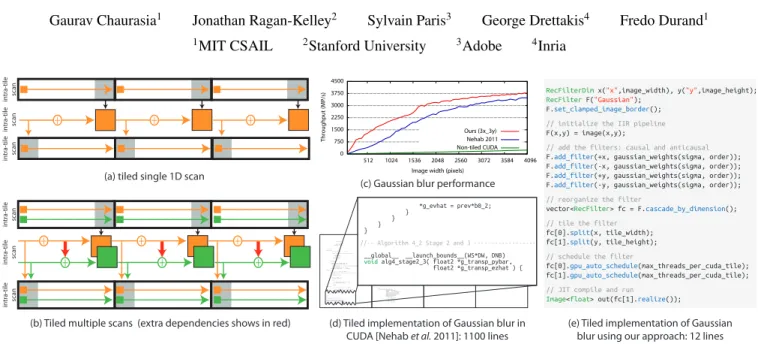
Figure 1: Tiling recursive filters exposes parallelism and locality in what are otherwise strictly-ordered computations. This improves their performance on highly parallel architectures like GPUs by an order of magnitude over traditional scanline-parallel implementations as shown in (c). This process converts them into multi-stage pipelines where some stages operate within tiles and some across tiles as shown in (a) and (b). Multi-filter pipelines get progressively more complex upon tiling because they induce extra dependencies shown by red arrows in (b) which makes these filters difficult to implement. (d) CUDA implementation of tiled 3rd-order recursive Gaussian blur requires 1100 lines of highly hand-optimized code [Nehab et al. 2011]. (d) Our compiler solves this problem by mechanizing the generation of tiled implementations and allows full user control over tiling and scheduling, making it easy for programmers to implement and experiment with different tiling strategies using only a few lines of code. The results show an order of magnitude better performance over commonly used scanline-parallel implementations and up to 1.4 times over hand tuned tiled implementations in 100 times less code.
Abstract
Infinite impulse response (IIR) or recursive filters, are essential for image processing because they turn expensive large-footprint convolutions into operations that have a constant cost per pixel regardless of kernel size. However, their recursive nature constrains the order in which pixels can be computed, severely limiting both parallelism within a filter and memory locality across multiple filters. Prior research has developed algorithms that can compute IIR filters with image tiles. Using a divide-and-recombine strategy inspired by parallel prefix sum, they expose greater parallelism and exploit producer-consumer locality in pipelines of IIR filters over multi-dimensional images. While the principles are simple, it is hard, given a recursive filter, to derive a corresponding tile-parallel algorithm, and even harder to implement and debug it.
We show that parallel and locality-aware implementations of IIR filter pipelines can be obtained through program transformations, which we mechanize through a domain-specific compiler. We show that the composition of a small set of transformations suffices to cover the space of possible strategies. We also demonstrate that the tiled implementations can be automatically scheduled in hardware-specific manners using a small set of generic heuristics. The pro-grammer specifies the basic recursive filters, and the choice of trans-formation requires only a few lines of code. Our compiler then generates high-performance implementations that are an order of magnitude faster than standard GPU implementations, and outper-form hand tuned tiled implementations of specialized algorithms which require orders of magnitude more programming effort—a few lines of code instead of a few thousand lines per pipeline.
CR Categories: I.3.1 [Computer Graphics]: Hardware Architecture—Parallel processing I.3.6 [Computer Graphics]:
Methodology and Techniques—Languages I.4.6 [Image process-ing and computer vision]: General—Image processprocess-ing software Keywords: Image processing, IIR filter, GPU computation, paral-lelism, memory locality, compiler, domain-specific language, high performance.
1
Introduction
Many image processing operations use stencils with large kernels, such as Gaussian or box blur, or local histograms [Chen et al. 2007; He et al. 2013]. With current image resolutions, kernels covering thousands of pixels or more are common and the quadratic growth of computation with respect to kernel width becomes unacceptable. Recursive or IIR filters are invaluable in reusing the computation from previous pixels and giving constant per pixel asymptotic com-plexity [Huang et al. 1979; Deriche 1993; Weiss 2006; Perreault and H´ebert 2007]. Unfortunately, this introduces sequential depen-dencies between pixels and severely limits parallelism. To address this, recent work shows how to manually decompose the compu-tation of a linear recursive filter across image tiles [Nehab et al. 2011]. Similar to prefix sum, filters are turned into multiple passes of intra-tile and inter-tile computation. This must be done across
multiple dimensions and computation across dimensions must be interleaved intelligently for locality. These algorithms achieve an order of magnitude speedup on highly-parallel architectures such as GPUs but also dramatically increase implementation complexity. So far, algorithms have been demonstrated for specific cases, such as summed area tables and Gaussian blur [Nehab et al. 2011], but each new filter or sequence of filters, depending on their order and causality, requires a new implementation of hundreds to thousands of lines to achieve state-of-the-art performance.
In this work, we dramatically simplify the implementation of high-performance tiled recursive filter pipelines using a domain-specific language (DSL). The user only needs to write the basic non-tiled linear recursive filters and a few lines describing the optimization strategy (Fig. 1e). The compiler generates code competitive with the best hand-tuned implementations, and surpasses pipelines built from individually optimized components.
Alternatively, one could imagine a library of a few hand-optimized building blocks. However, the composition of optimized kernels is suboptimal because it misses on opportunities to perform global op-timization. For any image processing pipeline, global optimization can significantly improve locality between pipeline stages [Ragan-Kelley et al. 2012]. Additionaly, recursive filters can be reorganized for improved efficiency. For example, Nehab et al. [2011] explored different strategies for a 2D 3rd order filter and found that rewriting it as 2nd order followed by 1st order filter was most efficient. In tra-ditional languages, each of these strategies requires a new intricate implementation.
Rather than requiring the programmer to implement a new algorithm for each strategy in each pipeline, we show that all such implementa-tions can be obtained by the mechanical application of a few simple program transformations. We distinguish two types of transforma-tions. First, we introduce a domain-specific language for recursive filter pipelines and a set of transformations that split the compu-tation into tiles and reorder the resulting passes. Second, given a set of passes, we build upon the Halide language to organize the actual computation i.e. mapping each operation to GPU kernels [Ragan-Kelley et al. 2012]. However, the large number of passes result in complex Halide pipelines, requiring the user to understand and decide hardware-specific parameters for each pass manually, which we refer to as scheduling. This would bring back the com-plexity we seek to alleviate. To address this, we present high level abstractions of tiled computation and use this with a generic set of heuristics to automatically schedule the complete pipeline for different hardware. Our heuristics automatically handle low-level details; we require programmer intervention only for high-level ex-perimentation with different tiling strategies. We demonstrate that our automatic schedules outperform previous work on tiled recursive filters [Nehab et al. 2011] and non-tiled CUDA implementations by an order of magnitude.
Contributions
• We describe a set of program transformations to optimize multi-dimensional linear recursive filters of arbitrary order on parallel architectures.
• We present a complete set of heuristics to automatically schedule arbitrarily complex tiled implementations for CPUs and GPUs. • Using the above, we present a compiler that dramatically simplifies
the implementation of high-performance IIR filter pipelines. Our results are an order of magnitude faster than commercial im-plementations that use traditional IIR filter algorithms, such as NVIDIA’s Thrust [Thrust 2015], and match or outperform hand-optimized implementations of tiled algorithms [Nehab et al. 2011], in orders of magnitude less code (Fig. 1(e)).
2
Previous work
In its most generic form, a recursive filter computes the output at any pixel from the output at the previous pixel by applying a constant number of mathematical operations. Many common image processing operations can be cast as recursive filters. Box filters can be computed in constant time using summed-area tables [Crow 1984]. Deriche [1993] describes a recursive filter approximation to Gaussian blur. Gaussian blur can also be approximated by repeated box filters [Rau and McClellan 1997]. A recursive formulation for histogram computation has been used for fast median filtering [Huang et al. 1979; Weiss 2006; Perreault and H´ebert 2007]. These filters serve as building blocks for more complex filters [Kass and Solomon 2010]. Traditionally, vendor optimized prefix sum [Thrust 2015] or summed area tables are cascaded to build more complex pipelines. Instead, we formulate an image processing pipeline as a series of filters and then optimize across the whole pipeline.
Parallel recursive filters IIR filters are not well suited for paral-lel hardware because they filter the input domain serially from one end to the other. Ruijters and Th´evenaz [2010] exploit parallelism between scanlines; this does not allow for sufficient parallelism for GPUs and results in poor memory locality because each thread has to read/write an entire scanline. Karp et al. [1967] and Kogge and Stone [1973] were the first to investigate parallelism in generic recurrence equations. Sung and Mitra [1986] and Blelloch [1989] describe the basic principles for exposing parallelism within a single 1D filter. Recent work has exploited this parallelism for GPUs focus-ing on memory locality and shared memory conservation [Hensley et al. 2005; Sengupta et al. 2007]. All these techniques compute a 1D filter along all scanlines and write the full image before computing the next filter. A pipeline involving n filters will read/write the full image n times, resulting in high memory bandwidth. Nehab et al. [2011] alleviate this issue in the specific cases of 2 and 4 filters using a tiling strategy. They split the image into 2D tiles, process each tile in parallel by all filters in shared memory and only write a subset of the result. They then apply inter-tile filtering passes to resolve all dependencies and add them to the intra tile result. This approach is restricted to 2D images for 1 or 2 filters per dimension. Kasagi et al. [2014] improve this strategy for up to 8% performance boost on summed area tables. Instead of describing different algorithms for different IIR filters pipelines, we present a small set of program transformations which can be used to programmatically transform any arbitrary pipeline into highly efficient tiled computation.
Domain-specific compilers Graphics has a long history of ex-ploiting domain-specific languages and compilers for easier access to high performance code. Most visible are shading languages [Han-rahan and Lawson 1990; Mark et al. 2003; Blythe 2006]. PARO [Hannig et al. 2008] presents partitioning techniques for automated hardware synthesis for massively parallel embedded architectures. Tangram [Chang et al. 2015] is a generic DSL that allows code portability across different architectures. Spiral in Scala [Ofenbeck et al. 2013] is a DSL for generating FFT implementations. Image processing languages also have a long history [Holzmann 1988; Elliott 2001; CoreImage 2006; PixelBender 2010]. Lepley et al. [2013] present a compilation approach for image processing for explicitly managed memory many-cores. Halide [Ragan-Kelley et al. 2013], HIPAcc [Membarth et al. 2015], Forma [Ravishankar et al. 2015], PolyMage [Mullapudi et al. 2015] are modern DSLs for im-age processing that enable code generation for multi-core CPUs and GPUs. They greatly simplify implementation of image processing operations, allowing the programmer to optimize across the whole pipeline. However these are limited to stencil operations, sampling and reductions, and they cannot parallelize recursive operations on the input domain. Most closely related to our focus on recursive filters, StreamIt [Thies et al. 2002; Gordon et al. 2002] optimizes
streaming and cyclostatic dataflow programs, specifically including transformation and optimization of chains of 1D recursive filters, but none have addressed the problem of extracting parallelism and locality from multi-dimensional recursive filters.
3
Overview
Our DSL sits on top of Halide [Ragan-Kelley et al. 2013]. Users first specify a series of IIR filters through a simple syntax (even simpler than pure Halide, see Sec. 4). Users can then reorganize the computation by optionally shuffling the order of filters (Sec. 5), and then specifying the tiling options (Sec. 6). These transformations generalize, abstract, and mechanize the strategies previously only demonstrated for a few specific examples in painstakingly handwrit-ten code [Nehab et al. 2011]. Finally, our compiler automatically maps the resulting tiled pipelines (Sec. 7) on to hardware, delivering state-of-the-art performance on a range of IIR filter pipelines from orders of magnitude simpler code (Sec. 8).
Our first transformation reorganizes filter computation. We exploit dimension separability and order invariance of IIR filters to shuffle different filters in a pipeline. Here, we allow the user to choose which filters to tile jointly (Sec. 5). For example, a sequence of 4 filters can be organized into groups of 2 filters each where filters in each group are tiled jointly. As shown in Sec. 5, these options lead to completely different implementations and have a significant impact on performance.
We then provide the split operator (Sec. 6). This applies our tiling transformations to filters defined on the full image, converting them into a series of filters that operate within image tiles, followed by filters across tiles, and then a final filter that assembles these two intermediate results and computes the final output. This tiling trans-formation exploits linearity and associativity of IIR filters. Internally, our compiler also makes critical performance optimization by mini-mizing back-and-forth communication between intra- and inter-tile computation and instead fuses computation by granularity level; e.g., we fuse all intra-tile stages because they have the same dependence pattern as the original non-tiled pipeline. This results in a compact internal graph of operations. We implement these transformations by mutating the internal Halide representation of the pipeline. Internally, our split operator mutates the original filters into a series of Halide functions corresponding to the intermediate opera-tions. We introduce automatic scheduling (Sec. 7), i.e. automatically mapping all the generated operations efficiently onto the hardware. We identify common patterns across the different operations and use heuristics to ensure memory coalescing, minimal bank conflicts for GPU targets, ideal thread pools, and unrolling/vectorization op-tions. We are able to do this without the hand-tuning or expensive autotuning required by general Halide pipelines because we can aggressively restrict our consideration to a much smaller space of “sensible” schedules for tiled recursive filters. Our heuristics sched-ule the entire pipeline automatically, which we show performs on par with manual scheduling. We also expose high-level schedul-ing operators to allow the user to easily write manual schedules, if needed, by exploiting the same restricted structure in the generated pipelines.
Filters defined in our language can be run directly, or combined with other Halide filters, preserving the ability to optimize across stages of a complex image processing pipeline, or interleaved with traditional C++/CUDA.
4
Recursive filter specification
We first describe the specification of recursive filter pipelines. Pro-grammers specify a filter pipeline F by its dimensions, input image,
and a set of recursive filters. In the example below, we first specify 2D index variables x and y, and initialize the filter by the input image In.
// Programmer definition
RecFilter F;
RecFilterDim x("x", width), y("y", height);
F(x,y) = In(x,y);
We maintain the internal representation as Halide functions (Func). A Func represents an image processing operation; the variables x, y represent a generic pixel x, y of the output image and the definition of the Func determines how the pixel must be computed. The original definition creates a Func object that is initialized by the input expression.
// Internal representation
Func R(F.name());
R(x,y) = In(x,y);
Unless the pipeline is tiled, it is represented by a single Func ob-ject. The pipeline can consist of multiple multi-dimensional filters. We provide an operator add filter that adds one filter at a time in a particular dimension. It specifies the filter dimension x, the causal/anticausal direction (+x or -x), and a list of linear feedfor-ward (first element of list) and feedback coefficients (remaining list elements).
F.add_filter(+x, {a0, a1, a2 ..});
Internally, this adds an update definition to the Func as follows:
RDom rx(0, image_width);
R(rx,y) = a0*R(rx,y) + a1*R(rx-1,y) + a2*R(rx-2,y)..;
The RDom represents bounded traversal in increasing order. It is different from variables like y because its bounds are known at compile time whereas the bounds of variables are inferred at runtime. Please refer to Halide documentation [Ragan-Kelley et al. 2012] for details. The update definition in the above code snippet updates the value at each pixel using the values of previous pixels, thereby creating a recursive filter or a scan. We create the recursive terms rx-1, rx-2in the dimension corresponding to x as indicated by add filter. The extent of the scan variable rx is the same as the extent of the corresponding dimension. The above initialization and update definition are equivalent to the following pseudo-code:
for all y do // initialize for all x do
f (x, y) ← In(x, y) end for
end for
for all y do // 1st filter or recursion or update definition for rx = 0 to image width − 1 do
f (rx, y) ← a0f (rx, y) + a1f (rx − 1, y) · · ·
end for end for
Please see supplemental material for a more detailed example of converting between our syntax, Halide code and pseudo-code. The tiling transformations (Sec. 6) mutate the original Func to com-pute its result from a directed acyclic graph of automatically gener-ated Func which form the intermediate stages of tiled computation. Programmers can add as many filters as needed to the recursive filter pipeline by calling add filter repeatedly. They can also explore different specifications of the same filter. For example, they can replace a 2nd-order filter with two 1st-order ones. They can perform these transformations manually (i.e., directly write two 1st-order filters), or use transformations to convert between higher- and lower-order filters which are already defined (shown next).
5
Overlapping and cascading IIR filters
An IIR filter pipeline is defined as a series of n IIR filters applied successively. These filters are separable along multiple dimensions, and the order in which multiple filters are applied in the same di-rection is immaterial. This means that a series of IIR filters can be reordered and recombined in different ways without affecting the result. They can be tiled jointly, or overlapped, such that all filters operate on image tiles simultaneously with different tiles being com-puted in parallel. Alternatively, a pipeline can be converted into two cascaded pipelines, with n0and n − n0overlapped filters such that the latter operates on the result of the former. Each pipeline reads/writes the full image once. Overlapping more filters saves full image reads/writes at the cost of more expensive intermediate opera-tions when tiling. Moreover, it is often useful to convert higher-order filters into multiple lower-order overlapped or cascaded filters. The optimal combination of filters to be overlapped must be determined empirically and is sensitive to input size and hardware. Rewrit-ing code for all these combinations is impractical for hand-written implementations.
We provide overlapping and cascading transformations that automat-ically convert between different alternatives. These transformations are applied on the non-tiled pipeline; they specify which filters to tile jointly. The generic cascade transformation takes a fully overlapped pipeline with n filters and creates a series of cascaded pipelines with subset of filters. For example, the following command converts the filter pipelines F into multiple cascaded filter pipelines, the first of which computes filters 0 to 3 of F, the second computes filters 4 and 6, the third computes 5 and 7 and so on.
F.cascade({0,1,2,3}, {4,6}, {5,7} ...);
Here, F is a non-tiled fully overlapped IIR filter pipeline. Internally, we represent it as a single Func containing each filter as an update definition (see Sec. 4). In the above example, we cascade this pipeline by extracting the first 4 update definitions (numbered 0 to 3) and adding them to a new Func that takes the original image as input. We then create another Func with update definitions numbered 4 and 6 from the original filter pipeline, that reads the output of the previous Func and so on. Each of the newly created Func is returned to the user as a RecFilter object that supports all the functionality as the original IIR filter pipeline. We use the reverse of this procedure to overlap multiple filters: we combine a series of cascaded pipelines F1, F2 etc. to create a new pipeline F that computes all the filters of constituent pipelines.
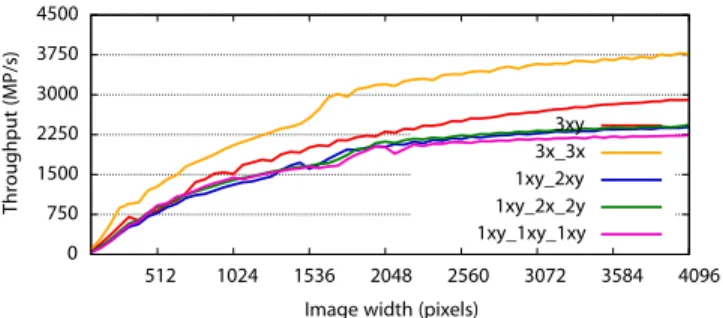
Converting between higher and lower order filters is more in-volved. Consider two cascaded filter pipelines A and B. We provide overlap filter ordertransformation that creates a new higher or-der filter pipeline equivalent to the original filters. We first compute a one-to-one mapping between the constituent filters of A and those of B by matching filter dimension and causality. The operation is only feasible if such a mapping can be found. We then use the z transform [Oppenheim and Schafer 2009] to compute the feedback and feedforward coefficients of each of new filter from those of the two original filters. For example, consider a 2D Gaussian filter that can be approximated by a 3rd order IIR filter decomposed into a causal and anticausal subsystem along both dimensions [van Vliet et al. 1998]. We compare the performance of different overlapping combinations in Fig. 2. The best performance comes from overlap-ping 3rd order filters in each dimension separately (code shown in Fig. 1(e)). This shows that the cascading vs. overlapping tradeoff cannot be resolved theoretically. In contrast, Nehab et al. [2011] found that cascading 2nd and 1st order was always better than 3rd order filters. This shows that overlapping options can be different depending upon hardware, which necessitates experimentation with the full range of alternatives.
0 750 1500 2250 3000 3750 4500 512 1024 1536 2048 2560 3072 3584 4096 Throughpu t(MP/s)
Image width (pixels)
3xy 3x_3x 1xy_2xy 1xy_2x_2y 1xy_1xy_1xy
Figure 2: Tradeoff between different overlapping options for 3rd order Gaussian filter. 3xy shows 3rd order filters overlapped inx andy, 3x 3y shows 3rd order filters overlapped in x and y sep-arately, 1xy 2xy shows cascaded 1st order and 2nd order filters overlapped inx and y, 1xy 2x 2y shows cascaded 1st order xy overlapped, cascaded with 2nd order overlapped inx and y sep-arately, 1xy 1xy 1xy shows 3 cascaded 1st order filters. 3x 3y gives the ideal tradeoff between cascading and overlapping. These hardware dependent results can only be determined empirically.
6
Tiling IIR filter pipelines
Given a pipeline of recursive filters specified as above, our goal is to mechanically transform it to enable high-performance parallel tiled computation. We provide a split operator to programmers and let them specify the tile size for each dimension to be split:
// programmer command
F.split(x, tile_width, y, tile_height ...);
This simple command triggers complex code transformations that generate new passes corresponding to intra- and inter-tile computa-tion. Recursive filters are characterized by their feedforward coeffi-cients and feedback coefficoeffi-cients. The new passes generated by the splitoperator are also recursive filters: either operating on pixels within tiles or on intermediate results across tiles. The mathematical complexity of tiling lies in computing the feedback and feedforward coefficients of all these new passes to ensure that the end result is nu-merically equivalent to the original filter. Since we seek to generate these operations automatically, our main challenge is to implement tiling as a set of code transformations so that it can be mechanized by a compiler aside from the mathematical derivation of all filter co-efficients. In this section, we focus on code transformations because that is the main contribution of our work. We delegate coefficient derivation to supplemental material; this is an extension of previous work [Kogge and Stone 1973; Blelloch 1989; Nehab et al. 2011] that computes filter coefficients for all stages of tiled computation for generic IIR pipelines.
We use a procedural approach for transforming the original filter code into tiled stages. We tile all the filters of the pipeline one by one, adding new stages of computation if required. To gain intuition, we first discuss the case of a single 1D filter before looking at multiple filters in the same dimension and finally generalize to multiple dimensions. We also begin with only causal filters and explain anticausal filters at the end.
6.1 Tiling a single 1D filter
We start by decomposing a 1D recursive filter R of order k that traverses the data in causal order, i.e., in the order of increasing indices. We represented it internally as a Func:
// Internal representation of a IIR filter
RDom rx(0, image_width), rk(0, k);
R(x) = I(x);
(a) naive 1D computation step 1 intra-tile scan one single global scan + + + + + + (b) tiled 1D computation step 3 intra-tile scan with tails step 2 inter-tile scan on tails only
Figure 3: Single 1D filter. (a) Naive sequential computation. (b) We transform it into a tiled scheme to improve performance. Step 1: we perform a scan on each tile in parallel. Step 2: we update the tails (the last elements of each tile) in order. Because of the order constraint, we cannot parallelize it; this is a fast operation nonetheless because of the small number of elements touched. Step 3: we update each tile in parallel to get the final result.
where, a is the list of feedback coefficients rx loops along the full row and rk loops from 0 to k. Assume the filter is tiled in x di-mension. As is known from previous work [Blelloch 1989], the above filter can be tiled to generate an identical intra-filter that only operates within image tiles, an inter-tile filter that aggregates the tailsof each image tile across all tiles and a final term that adds the aggregated or completed tails to the intra-tile filtering result from the first stage (see Fig. 3). The tail refers to the last k elements of each tile; the first element of each tile needs some contribution from the last k elements of the previous tile which is provided by the tail. We now describe the procedure to create the above subfunctions.
Intra-tile subfunction We create an intra-tile subfunction by di-rectly mutating the original filter definition. We first replace the tiled dimension x by an intra-tile index xi and an inter-tile index xo. In the update definition, we restrict the recursion to image tiles by replacing rx with rxi and tile index xo, where rxi loops from 0 to tile width.
// Internal definition of first intra-tile Func // Each tile xo is independent, thus parallelizable
RDom rxi(0, tile_width);
R_intra(xi, xo) = I(xo*tile_width+xi);
R_intra(rxi,xo) = sum(a(k) * R_intra(rxi-rk,xo));
Note that the above operation is independent in tile index xo. It can therefore be computed in parallel across tiles (Fig. 3 step 1).
Tail subfunction The intra-tile results are incomplete because they do not have contributions from any preceding tile. We then extract the tail of the intra-tile result. The tail of each tile is the residual that must be added to the subsequent tile in order to complete its result.
// Internal definition of tail of each tile
R_tail(xi, xo) = R_intra(tile_width-1-xi, xo);
Inter-tile subfunction The tails extracted from each tile do not have any contribution from any of the previous tiles. We complete the tails by aggregating them across tiles (Fig. 3 step 2). We implement this as a 1st order IIR filter R ctail that is a recursion over tail elements across tiles. We create a new scan variable rxo that loops over all tiles. The feedback coefficients are contained in a matrix P whose derivation can be found in supplemental material (Sec. 2.1, 3) or in previous work [Nehab et al. 2011]. This filter is serial; it is nonetheless fast because it touches only tail elements from each tile. We refer to the result of this subfunction as completed tails.
// Internal def. of inter-tile filter across tiles
RDom rxo(0, image_width/tile_width);
R_ctail(xi,xo) = R_tail(xi,xo);
{
{
{
+ + + + + + + 1 2 3 1 2 3 1 2 3 1 2 3(a) naive multiple 1D scans
(b) tiled multiple 1D scans step 1a
intra-tile scans one global scan per filter
step 3 intra-tile scan with tails step 2 inter-tile scans on tails only step 1b per-scan per-tile tails + + ++ + ++ + ++ +
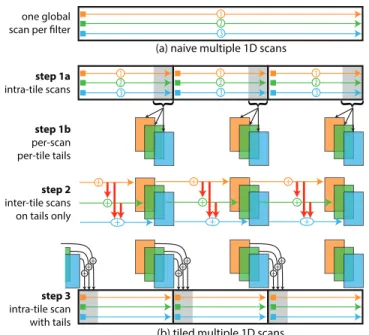
Figure 4: Mutliple 1D filters. (a) Naive sequential computation. One can apply the single-filter scheme (Fig. 3b) once per filter but this does not fully exploit the locality of operations. (b) We treat all filters at once to minimize alternation between intra- and inter-tile steps. Step 1a: we apply all filters within each inter-tile in parallel. Step 1b: we save a copy of the tails after each filter. Step 2: we sequentially update the tails using the tails of all the preceding filters at the previous tile. Step 3: we update each tile in parallel using all the tails at the previous tile to get the final result (step 3).
R_ctail(xi,rxo) += P(tile_width-1-rk) * R_ctail(rk,
rxo-1);
Final intra-tile subfunction The previous inter-tile filter com-pletes the tail of each tile which can now be added to the intra-tile result of the subsequent tile. To this end, we create a verbatim copy of the R intra from the first stage. We then mutate it to initialize it with the input image, plus the contribution tail of the previous tile (Fig. 3 step 3). We then apply the intra-tile filter as in R intra.
// Internal definition of final result computation // Extra update def to all tail of previous tile
R_final(xi, xo) = I(xo*tile_width+xi);
R_final(rk, xo) = P(rk) * R_ctail(rk,xo-1);
R_final(rxi,xo) = sum(a(rk) * R_final(rxi-rk,xo));
We finally modify the original function to read the final result from R final.
// Convert x to xi and xo using div and mod
R(x) = R_final(x%tile_width, x/tile_width);
6.2 Multiple 1D filters along the same dimension
We have described basic code transformations for a single IIR filter. We will use the above transformations as building blocks to give an intuitive description for more complex cases. We avoid giving exact code snippets to keep the description terse.
Consider n IIR filters on the same dimension. We tile them jointly using the same principle as above. This time we generate (a) single intra-tile subfunction for first stage, (b) n different tail subfunctions, (c) n different inter-tile subfunctions, and (d) single final intra-tile subfunction to compute the full result from the input image and n completed tails.
The first stage intra-tile subfunctions is generated the same way as in Sec. 6.1, except that the subfunction now has one update definition for each of the n IIR filters (Fig. 4 step 1a). The n tail subfunctions extract the tail of each tile after each of the n IIR filters are applied by the intra-tile subfunction of the first stage. This gives n different tails corresponding to the n filters (Fig. 4 step 1b). Similarly, the n inter-tile filters are all 1st order filters on the tails of each of the original n IIR filters (Fig. 4 step 2), except that the j-th inter-tile subfunction has to be initialized by the j-th tail subfunction as well as the j − 1-th inter-tile subfunction. The coefficients for each j-th filter are stored in j-th row of the matrix P whose derivation is given in supplementary material.
// Extra dependency from completed tail of previous // filter of the same dimension
R_ctail[j](xi,xo) = R_tail[j](xi,xo) +
P(j,tile_width-1-rk) * R_ctail[j-1](xi,xo-1);
R_ctail[j](xi,rxo) += P(j,tile_width-1-rk) *
R_ctail[j](rk,rxo-1);
This is the only new cross-filter dependency induced by multiple filters. The final stage subfunction has to be initialized by the tails of n different inter-tile filters (Fig. 4 step 3) instead of just 1 in Sec. 6.1.
Discussion The above clearly shows the computational expense added by multiple filters. Much like the non-tiled counterpart, the intra-tile subfunctions have to compute more filters. The extra slowdown is due to computation of more inter-tile filters. As a result, joint-tiling of n IIR filters can be more expensive than joint tiling of cascaded groups of n0and n − n0(n0< n). Our compiler allows convenient experimentation with different tiling combinations as explained in Sec. 5.
6.3 Multiple filters along different dimensions
We now generalize to multiple filters in multiple dimensions. We use the same basic principles as in the previous two cases and apply them to generate a single intra-tile first stage and a separate tail for each filter irrespective of the dimensions (Fig. 5) steps 1a, 1b). We create inter-tile subfunctions for each of the tail subfunctions that loop over all the tile in their respective dimensions (Fig. 5 steps 2, 3b) accounting for cross-filter dependencies exactly as in Sec. 6.2. The final intra-tile term is also an extension of the one in Sec. 6.2; we add the tail from each filter in each dimension to the intra-tile result before applying the particular intra-tile scan.
The critical difference is the introduction of cross-dimensional de-pendencies (Fig. 5 steps 3a). All the tails in the l-th dimension require some contribution from completed tails in all previous di-mensions. To this end, we create one intra-tile subfunction as a verbatim copy of the first stage for each dimension. We mutate its definition such that it gets initialized by the completed tails of the corresponding dimension, say x. We then remove all scans from this subfunction on any dimension preceding x. This now becomes an intra-tile subfunction that reads the tails of the x dimension and applies all IIR filters of subsequent dimensions. The cross dimension dependency of any other dimension y with respect of x is the result of the newly created intra-tile subfunction after applying all IIR filters of all dimensions between x and y, including y and excluding x.
We then initialize the inter-tile subfunction of each filter of each dimension using (1) the tail of that filter in that dimension, (2) one cross-filter dependency term i.e. the completed tail of the previous filter in the same dimension, and (3) cross-dimensional dependency with respect to each preceding dimension.
Anticausal filters Anticausal filters process data in the reverse or-der: right to left, or bottom to top. We handle them by using reverse
pixel indices tile width-1-xi and tile width-1-rxi instead of xiand rxi respectively for intra-tile subfunctions. Similarly, we use reverse tile indices for inter-tile subfunctions.
It is clear that the complexity of the tiled implementations grows quickly as the number of filters increases. Our procedural approach in Sec. 6.2, 6.3 mechanizes the complete procedure.
7
Automatically scheduling tiled pipelines
As introduced in Sec.1, scheduling refers to determining hardware specific parameters for actual computation of each filter. Our tiling transformations create a relatively large number of sub-functions for a given pipeline, each representing one stage of computation, all of which have to be scheduled for efficient execution. All are maintained as Halide Funcs and can be scheduled with total free-dom using Halide’s existing scheduling language. However, this is challenging because the number of subfunctions can be large and scheduling them individually requires intimate knowledge of the generated structure and the operations being performed.
Because of the more restricted domain of tiled recursive filter pipelines relative to arbitrary Halide, we can instead automatically schedule the generated pipelines for efficient GPU execution, with no programmer intervention. In this section we present the scheduling strategy applied by our compiler. The end result is an automati-cally scheduled pipeline for both CPUs and GPUs that matches or outperforms the best hand-tuned code in all our tests.
High-level semantics The tiling transformations generate sub-functions of two classes: intra- and inter-tile (Sec. 6). We tag all subfunctions with either of these classes to make selective schedul-ing decisions afterwards.
Each function is composed of multiple dimensions; we associate metadata with each dimension. We mark the dimension undergoing a serial scan as SCAN for each function. All within-tile pixel indices are marked INNER and tile indices are marked OUTER . Functions may also have non-tiled dimensions, e.g., a filter that is tiled only along rows but not along columns. We split these logically into an INNERand OUTER dimension using Halide’s split operator. This reduces all dimensions to INNER and OUTER and scheduling heuristics need to account only for these two cases. We define all heuristics on these high-level handles and use them to retrieve functions and dimensions for applying specific scheduling operators.
We now describe scheduling heuristics starting from high-level deci-sions regarding compute granularity of functions to details such as unrolling etc. We implement these internally using Halide’s schedul-ing operators: compute root, compute at, reorder, parallel, reorder storage, split, vectorize and unroll.
Global vs local storage The most important high-level schedul-ing choice is to decide whether to compute and store a function in global memory so that it is always available to consumers or recom-pute it on demand locally within consumer loops. Local computation amounts refers to shared memory for GPUs. Intra-tile subfunctions involve a bounded loop over pixels within a tile and their compute footprint is larger than output size because they compute over the full tile or more but only store the last row/column as tail (see Fig. 4, 5 step 1). We therefore compute them in local memory to avoid global memory bandwidth. On the other hand, inter-tile subfunc-tions have multiple consumers and they require a variable sized scan over all image tiles leads to variable local memory requirements; we compute these in global memory.
Loop nest order Each Func results in a loop nest, one loop for each dimension. The loops can be reordered without changing the
+ + step 1a
intra-tile scans per-scan per-tile per-dimension tailsstep 1b inter-tile scans on x tailsstep 2
step 3b inter-tile scans on y tails step 3a
intra-tile scans on x tails
+ + + + + + + + + + + + + + step 4
intra-tile scans with tails from all dimensions
+ + + + + + + + + + + + + + + + + + + + + + + + + + + + + + + + + + + + + + + + + +
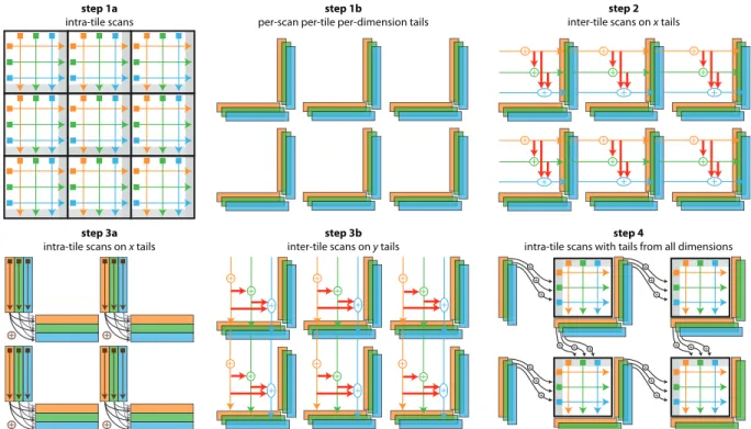
Figure 5: Multiple 2D filters. Step 1a: we compute all filters within each tile in parallel. Step 1b: we copy the tails after each filter. Step 2: we complete the tails of all the filters along thex dimension using the 1D case as in Fig. 4. Step 3a: to account for cross-dimensional residuals, we apply they filters on all x tails (vertical arrows) and incorporate these into all the y tails (corner arrows). Step 3b: we use these residuals to complete they tails. Step 4: we compute the final result using the completed tails of previous tiles from all filters.
computation, but have a significant effect on performance. We spec-ify SCAN variables as innermost loops, followed by INNER variable loops which iterate over pixels within tiles, followed by OUTER vari-able loops. This keeps all serial computation innermost and all outer loops can be parallelized.
Parallel threads For GPU targets, me map all OUTER variables to CUDA tiles and the first two INNER variables to CUDA threads. Choosing two innermost INNER variables ensures a reasonable num-ber of threads; this leads to O(t2) threads for intra-tile subfunctions and O(t) threads for inter-tile subfunctions, where t is the tile width. The user indicates the maximum number of threads in each tile. If the number of threads launched above is more than the threshold, we logically split the second INNER variable by a factor that retains the correct number of threads and unroll the rest. If the number of threads is less than the threshold, we launch extra threads per tile by running multiple image tiles in each CUDA warp. To this end, we split an OUTER variable and map one of the new variables to CUDA warps and other to CUDA threads. For CPU targets, we place the outermost OUTER variable in the job queue for potential parallel execution. This offers sufficient parallelism; there is no need for parallelization of other dimensions.
Memory coalescing Memory coalescing ensures that parallel
threads read and write from adjacent memory locations for GPUs. We use two heuristics: (a) we choose packed storage for dimensions mapped to parallel threads, and (b) we choose OUTER dimenisons to be stored outermost, i.e. wigh maximum stride. While (a) is obvious, (b) ensures that the storage of OUTER dimensions does not add more strides in the storage of any INNER dimension, which may be parallelized. In practice, we list all dimensions and sort them according to the above heuristics. We then transpose the multi-dimensional output buffer as per the desired ordering.
Vectorization For CPUs, we vectorize the innermost INNER
dimen-sion if it is packed contiguously in memory. We split this dimendimen-sion by a factor of 8 or 16 and vectorize the newly created dimension.
Loop unrolling We place the loop over any SCAN variables just outside any vectorized dimensions and unroll them for both CPU and GPUs. These loops compute the recurrence equation of the filter; their body is small enough to be unrolled without incurring instruction cache misses or bloating code size.
Bank conflicts Intra-tile operations to be computed in GPU shared memory can suffer from bank conflicts. We solve this by allocating (w + 1) × h to compute w × h pixels in shared memory; the extra column swizzles the mapping of pixels to banks. Consider an intra-tile operation represented by A(xi, xo, yi, yo ..). We add an extra update definition that adds one extra 1 pixel to the innermost INNERdimension.
A(xi, xo, yi, yo ..) = original_definition
A(tile_width, xo, yi, yo ..) = 0; // padding
With the OUTER dimensions mapped to CUDA tiles, the required shared memory is equal to the product of extents of all INNER vari-ables. Padding the innermost of these variables increases the shared memory allocation by one column. Thus, a simple code trans-formation resolves an issue which most applications handle using convoluted CUDA code.
Manual control Precise knowledge of computation pattern allows the compiler to apply the same heuristics as a programmer would apply, which allows our heuristics to match hand tuned schedules. However, heuristics may become outdated as the hardware changes. Our abstraction still provides a terse and intuitive approach for scheduling. In fact, we have implemented our heuristics using the same high-level handles within 100 lines of code for both CPU and GPU targets within the compiler. This portable scheduling code can be easily changed in the future without touching tiling and other
transformations.
8
Results
We present results on a variety of image filtering operations ex-pressed as recursive filter pipelines. We compare our performance with commercial non-tiled implementations taken from CUDA toolkit [NVIDIA 2015] and the tiled implementations of Nehab et al. [2011]. Our fully automatic results match hand tuned tiled versions and outperform commercial libraries like NVIDIA Thrust by an order of magnitude. We demonstrate that reorganizing com-putation in larger pipelines allows significant performance gains compared to hand tuned implementations used as black boxes. We also demonstrate CPU results for very large 1D arrays with high order filters. All our examples require 10-15 lines of code while previous work requires 100-200 and 500-1100 lines of CUDA for non-tiled and tiled implementations respectively.
We profiled GPU code using NVIDIA’s profiler on a GeForce GTX Titan. We use 32-bit floating point arithmetic for all experiments. Runtimes are averaged over 1000 iterations.
0 2000 4000 6000 8000 10000 12000 512 1024 1536 2048 2560 3072 3584 4096 Throughpu t(MP/s)
Image width (pixels)
Ours Nehab 2011 NVIDIA Thrust
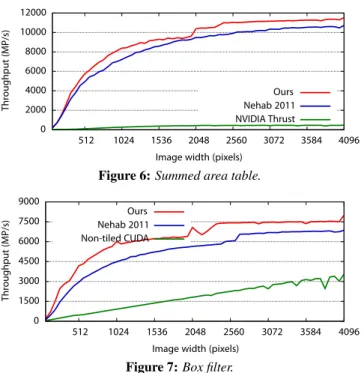
Figure 6: Summed area table.
0 1500 3000 4500 6000 7500 9000 512 1024 1536 2048 2560 3072 3584 4096 Throughpu t(MP/s)
Image width (pixels) Ours
Nehab 2011 Non-tiled CUDA
Figure 7: Box filter.
Our summed area table is slightly faster than Nehab et al. [2011] and 10 times faster than NVIDIA Thrust (Fig. 6). Thrust also has no support for higher order or multi-dimensional filtering. We inherit the same speedup margin over Nehab et al. [2011] for box filter implemented using summed area table (Fig. 7). A scanline-parallel recursive box filter using CUDA is 2-2.5 times slower. The state-of-the-art summed area table by Kasagi et al. [2014] is 8% faster than Nehab et al. [2011], which is on par with our results.
Our tiled implementations are slightly faster than Nehab et al. [2011] because we use better loop unrolling within CUDA tiles and launch an appropriate number of threads. Our scheduler can adapt these numbers for any GPU with a single parameter - CUDA thread block size. An identical schedule should allow Nehab et al. [2011] to match our results but modifying the CUDA warps and loop unrolling can be cumbersome and error-prone.
We implemented bicubic B-spline interpolation as a pair of causal and anticausal 1st order filters along rows and columns. Our results in Fig. 8 show that we are an order of magnitude faster than non-tiled implementation. We trail the tiled CUDA implementation because
0 1500 3000 4500 6000 7500 9000 512 1024 1536 2048 2560 3072 3584 4096 Throughpu t(MP/s)
Image width (pixels)
Ours Nehab 2011 Non-tiled CUDA
Figure 8: Bicubic interpolation using 1st order causal-anticausal filter pairs. We are an order magnitude faster than a non-tiled implementation but trail Nehab et al. [2011] slightly because we require more shared memory.
we require t(t + nk + 1) numbers in shared memory whereas hand tuned CUDA requires t(t + 1) where t is tile width, n is number of IIR filters and k is filter order (counting bank conflict resolution in both cases). The extra memory is required to copy out the tails after each intra-tile filter (Sec. 6.2, Fig. 4). This is a Halide design issue which may be alleviated in the future.
However, this does not restrict our performance for more complex filters. As the filter order or number of filters grows, fully overlapped solutions may become suboptimal and it is often faster to use a cascaded pipeline even though it entails more I/O (Fig. 2).
0 750 1500 2250 3000 3750 4500 512 1024 1536 2048 2560 3072 3584 4096 Throughpu t(MP/s)
Image width (pixels)
Ours (3x_3y) Nehab 2011 Non-tiled CUDA
Figure 9: Gaussian blur [van Vliet et al. 1998].
We use a 3rd order IIR filter decomposed as a causal-anticausal pair to approximate Gaussian blur [van Vliet et al. 1998]. We im-plemented 5 different reorganizations of the 3rd order IIR filters including cascading along dimensions, splitting into lower filter or-ders etc. (Fig. 2). Here we compare our best variant, a cascade of 3rd order filters along rows and then along columns, to previous work (Fig. 9). Nehab et al. [2011] found that 3rd orders filters are better implemented as 1st and 2nd order filters. This was not true in our tests which we believe is because of difference in hardware. Our approach allows programmers to easily experiment with all the variants and select the best. We outperform scanline-parallel non-tiles CUDA implementations by an order of magnitude. Almost all real world applications use the non-tiled version, partly because it is easy to implement. Our approach is just as easy to use as shown in Fig 1(e) and much faster.
We notice greater performance gains for larger pipelines such as 3 iterated box filters (see Fig. 10). Repeated applications of a sin-gle box filter decreases the throughput of non-tiled and Nehab’s implementation linearly. Instead, we reorganize the computation: we compute a single box filter followed by a double box filter. The double box filter itself is computed using a cascade of 2nd order filter along rows and along columns. Our speedup comes from the fact that we require 5 read/writes of the image while thrice repeated application of a box filter entails to 6 image read/writes. Note that we could also fuse the last step of one filter pipeline with the first stage of the next filter pipeline to somewhat reduce I/O. We chose
0 500 1000 1500 2000 2500 3000 512 1024 1536 2048 2560 3072 3584 4096 Throughpu t(MP/s)
Image width (pixels) Ours
Nehab 2011 Non-tiled CUDA
Figure 10: Box filter (3 iterations). Our performance gain results from intelligent reorganization of computation instead of repeated application as in previous work.
not to implement this because this resulted in one merged stage which needed twice the shared memory and interfered with our bank conflict management. We would like to resolve this in future work. We could also compute 3 box filters directly using a 3rd order xy overlapped integral image but this becomes numerically unstable. We use 2nd order IIR filters along a single dimension only, as this is numerically stable with 32-bit floats.
0 500 1000 1500 512 1024 1536 2048 2560 3072 3584 4096 Throughpu t(MP/s)
Image width (pixels)
Ours Nehab 2011
Figure 11: Difference of Gaussians using 3 box filters Lastly, we demonstrate difference of Gaussians. We approximate each Gaussian using 3 box filters in Fig. 11. This involves computing two Gaussians with different variances and subtracting them. We use the methodology described above to optimize the box filters used for computation. Additionally, we notice that the entire pipeline is identical for both the Gaussians. We therefore compute them in the same GPU kernels for an extra performance boost. Our implementation requires 10 image read/writes and 13 GPU kernels as opposed to 13 read/writes and 25 kernels for Nehab et al. [2011]. Such optimization is not feasible with precompiled libraries.
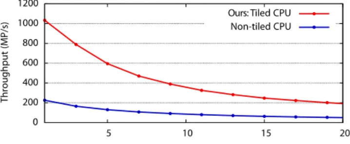
Tiling 1D filters on CPUs Most CPU architectures can extract sufficient parallelism from independent scanlines in 2D image filters, but 1D recursive filters are still severely constrained by the lack of parallelism. We demonstrate the first tiled and parallelized imple-mentations of higher order recursive filters on 1D input. Such filters are useful in the broader signal processing community [Stearns and Hush 2002]. Using an 8 core Intel 3.5 GHz machine with 8GB RAM on 32-bit float data, our results in Fig. 12 show that tiled implemen-tations are 3.5-5 times faster than a non-tiled implemenimplemen-tations. High order filters can be hard to design and can be numerically unstable [Stearns and Hush 2002]; these are frequently implemented as a series of 2nd order filters. Joint tiling of multiple overlapped 2nd order filters is up to 5.5 times faster (Fig. 13).
We also observe that the runtime of 12 overlapped filters is 125.6 ms while the runtime of 6 overlapped filters is 58.7 ms. This suggests that cascading two 6-overlapped pipelines will perform better than a single 12-overlapped pipeline. We allow the programmer to easily explore these reorganization alternatives (Sec. 5).
0 200 400 600 800 1000 1200 5 10 15 20 Throughpu t(MP/s) Filter order
Ours: Tiled CPU Non-tiled CPU
Figure 12: High order 1D filter on 100 million numbers.
0 100 200 300 400 500 600 3 6 9 12 15 Throughpu t(MP/s)
Number of overlapped filters
Ours: Tiled CPU Non-tiled CPU
Figure 13: Overlapped 2nd order 1D filters on 100 million numbers.
9
Conclusions
We have presented a DSL and compiler for automatically optimizing recursive filter pipelines. The main contribution is automatic tiling of generic pipelines achieved by a set of simple code transformations. This relieves the programmer from the tedium of mathematical derivation and implementation of different tiling variations of the same filter. We present high level abstractions and heuristics which we use to schedule the internally generated graph of tiled operations. The end result is a completely automatic solution for recursive filters, making it as easy to use as libraries like NVIDIA Thrust, but an order of magnitude faster. Programmers can merge and schedule tiled recursive filters with other stages of a larger image processing pipelines to explore optimization strategies not feasible with vedor-provided libraries.
Our results show that tiling is beneficial on both CPUs and GPUs. We outperform vendor provided non-tiled implementations by 5-10 times and match complicated hand-tuned tiled implementations of Nehab et al. [2011] with only 10 lines of simple code compared to 500-1100 lines of CUDA. For larger filter pipelines such as dif-ference of Gaussians, we outperform Nehab et al. [2011] by up to 1.8 times because of our ability to explore different filter tiling alternatives and optimize across the entire image processing pipeline. We demonstrate 5 times performance boost on CPUs for pipelines consisting of multiple high order filters for large 1D data.
Altogether, our system enables programmers to quickly write ef-ficient implementations of filter pipelines and optimize across the whole pipeline. We hope this will help rethink how image processing pipelines are programmed.
References
BLELLOCH, G. E. 1989. Scans as primitive parallel operations. IEEE Transactions on Computers 38, 11 (Nov), 1526–1538. BLYTHE, D. 2006. The Direct3D 10 system. ACM Trans. Graph.
25, 3 (July), 724–734.
M. W. HWU, W. 2015. Tangram: a high-level language for performance portable code synthesis. In Programmability Issues for Heterogeneous Multicores.
CHEN, J., PARIS, S.,ANDDURAND, F. 2007. Real-time edge-aware image processing with the bilateral grid. ACM Trans. Graph. 26, 3 (July), 103:1–103:9.
COREIMAGE, 2006. Apple CoreImage programming guide. https://developer.apple.com/library/ ios/documentation/GraphicsImaging/Conceptual/ CoreImaging/ci intro/ci intro.html.
CROW, F. C. 1984. Summed-area tables for texture mapping. In SIGGRAPH, 207–212.
DERICHE, R. 1993. Recursively implementating the Gaussian and its derivatives. Tech. Rep. RR-1893, INRIA.
ELLIOTT, C. 2001. Functional image synthesis. In Proceedings of Bridges.
GORDON, M. I., THIES, W., KARCZMAREK, M., LIN, J., MELI, A. S., LAMB, A. A., LEGER, C., WONG, J., HOFFMANN, H., MAZE, D.,ANDAMARASINGHE, S. 2002. A stream compiler for communication-exposed architectures. In ASPLOS, 291–303. HANNIG, F., RUCKDESCHEL, H., DUTTA, H., ANDTEICH, J. 2008. PARO: Synthesis of hardware accelerators for multi-dimensional dataflow-intensive applications. In Reconfigurable Computing: Architectures, Tools and Applications, 287–293. HANRAHAN, P.,ANDLAWSON, J. 1990. A language for shading
and lighting calculations. In Computer Graphics (Proceedings of SIGGRAPH 90), 289–298.
HE, K., SUN, J.,ANDTANG, X. 2013. Guided image filtering. IEEE Trans. Pattern Anal. Mach. Intell. 35, 6, 1397–1409. HENSLEY, J., SCHEUERMANN, T., COOMBE, G., SINGH, M.,
ANDLASTRA, A. 2005. Fast summed-area table generation and its applications. Computer Graphics Forum 24, 3, 547–555. HOLZMANN, G. 1988. Beyond Photography. Prentice Hall. HUANG, T., YANG, G., AND TANG, G. 1979. A fast
two-dimensional median filtering algorithm. 13–18.
KARP, R. M., MILLER, R. E.,ANDWINOGRAD, S. 1967. The organization of computations for uniform recurrence equations. Journal of the ACM 14, 3 (July), 563–590.
KASAGI, A., NAKANO, K.,ANDITO, Y. 2014. Parallel algorithms for the summed area table on the asynchronous hierarchical mem-ory machine, with GPU implementations. In International Con-ference on Parallel Processing, 251–260.
KASS, M.,ANDSOLOMON, J. 2010. Smoothed local histogram filters. ACM Trans. Graph. 29, 4 (July), 100:1–100:10. KOGGE, P. M.,ANDSTONE, H. S. 1973. A parallel algorithm for
the efficient solution of a general class of recurrence equations. IEEE Transactions on Computers C-22, 8 (Aug), 786–793. LEPLEY, T., PAULIN, P.,ANDFLAMAND, E. 2013. A novel
com-pilation approach for image processing graphs on a many-core platform with explicitly managed memory. In International Con-ference on Compilers, Architecture and Synthesis for Embedded Systems (CASES), 1–10.
MARK, W. R., GLANVILLE, R. S., AKELEY, K.,ANDKILGARD, M. J. 2003. Cg: A system for programming graphics hardware in a C-like language. ACM Trans. Graph. 22, 3 (July), 896–907. MEMBARTH, R., REICHE, O., HANNIG, F., TEICH, J., KORNER,
M.,ANDECKERT, W. 2015. HIPAcc: A domain-specific lan-guage and compiler for image processing. IEEE Transactions on Parallel and Distributed Systems.
MULLAPUDI, R. T., VASISTA, V., AND BONDHUGULA, U. 2015. Polymage: Automatic optimization for image process-ing pipelines. In ASPLOS, 429–443.
NEHAB, D., MAXIMO, A., LIMA, R. S.,ANDHOPPE, H. 2011. GPU-efficient recursive filtering and summed-area tables. ACM Trans. Graph. 30, 6 (Dec.), 176:1–176:12.
NVIDIA, 2015. NVIDIA CUDA toolkit. https://developer. nvidia.com/cuda-toolkit.
OFENBECK, G., ROMPF, T., STOJANOV, A., ODERSKY, M.,AND
P ¨USCHEL, M. 2013. Spiral in Scala: Towards the systematic construction of generators for performance libraries. SIGPLAN Not. 49, 3 (Oct.), 125–134.
OPPENHEIM, A. V.,ANDSCHAFER, R. W. 2009. Discrete-Time Signal Processing, 3rd ed. Prentice Hall Press.
PERREAULT, S., AND H ´EBERT, P. 2007. Median filtering in constant time. IEEE Trans. Img. Proc. 16, 9 (Sept.), 2389–2394. PIXELBENDER, 2010. Adobe PixelBender reference. http://www.
adobe.com/devnet/archive/pixelbender.html.
RAGAN-KELLEY, J., ADAMS, A., PARIS, S., LEVOY, M., AMA
-RASINGHE, S., AND DURAND, F. 2012. Decoupling algo-rithms from schedules for easy optimization of image processing pipelines. ACM Trans. Graph. 31, 4 (July), 32:1–32:12. RAGAN-KELLEY, J., BARNES, C., ADAMS, A., PARIS, S., DU
-RAND, F.,ANDAMARASINGHE, S. 2013. Halide: a language and compiler for optimizing parallelism, locality, and recomputa-tion in image processing pipelines. In PLDI, 519–530.
RAU, R.,ANDMCCLELLAN, J. 1997. Efficient approximation of Gaussian filters. IEEE Trans. Sig. Proc. 45, 2 (Feb), 468–471. RAVISHANKAR, M., HOLEWINSKI, J.,ANDGROVER, V. 2015.
Forma: A DSL for image processing applications to target GPUs and multi-core CPUs. In GPGPU, 109–120.
RUIJTERS, D.,ANDTHEVENAZ´ , P. 2010. GPU prefilter for accurate cubic b-spline interpolation. The Computer Journal.
SENGUPTA, S., HARRIS, M., ZHANG, Y., AND OWENS, J. D. 2007. Scan primitives for GPU computing. In Symposium on Graphics Hardware, 97–106.
STEARNS, S.,ANDHUSH, D. 2002. Digital Signal Processing with Examples in MATLAB, Second Edition. Electrical Engineering & Applied Signal Processing Series. Taylor & Francis.
SUNG, W.,ANDMITRA, S. 1986. Efficient multi-processor im-plementation of recursive digital filters. In IEEE Conference on Acoustics, Speech and Signal Processing, vol. 11, 257–260. THIES, W., KARCZMAREK, M.,ANDAMARASINGHE, S. P. 2002.
Streamit: A language for streaming applications. In International Conference on Compiler Construction, 179–196.
THRUST, 2015. NVIDIA Thrust. https://developer.nvidia. com/Thrust.
VANVLIET, L. J., YOUNG, I. T.,ANDVERBEEK, P. W. 1998. Recursive Gaussian derivative filters. In International Conference on Pattern Recognition, vol. 1, 509–514 vol.1.
WEISS, B. 2006. Fast median and bilateral filtering. ACM Trans. Graph. 25, 3 (July), 519–526.