HAL Id: insu-02305942
https://hal-insu.archives-ouvertes.fr/insu-02305942
Submitted on 4 Oct 2019
HAL is a multi-disciplinary open access
archive for the deposit and dissemination of
sci-entific research documents, whether they are
pub-lished or not. The documents may come from
teaching and research institutions in France or
abroad, or from public or private research centers.
L’archive ouverte pluridisciplinaire HAL, est
destinée au dépôt et à la diffusion de documents
scientifiques de niveau recherche, publiés ou non,
émanant des établissements d’enseignement et de
recherche français ou étrangers, des laboratoires
publics ou privés.
Time-stamp correction of magnetic observatory data
acquired during unavailability of time-synchronization
services
Pierdavide Coisson, Kader Telali, Benoit Heumez, Vincent Lesur, Xavier
Lalanne, Chang Jiang Xin
To cite this version:
Pierdavide Coisson, Kader Telali, Benoit Heumez, Vincent Lesur, Xavier Lalanne, et al.. Time-stamp
correction of magnetic observatory data acquired during unavailability of time-synchronization
ser-vices. Geoscientific Instrumentation, Methods and Data Systems Discussions, European Geosciences
Union 2017, 6 (2), pp.311-317. �10.5194/gi-6-311-2017�. �insu-02305942�
https://doi.org/10.5194/gi-6-311-2017
© Author(s) 2017. This work is distributed under the Creative Commons Attribution 3.0 License.
Time-stamp correction of magnetic observatory data acquired
during unavailability of time-synchronization services
Pierdavide Coïsson1, Kader Telali1, Benoit Heumez1, Vincent Lesur1, Xavier Lalanne1, and Chang Jiang Xin2 1Institut de Physique du Globe de Paris, Sorbonne Paris Cité, Université Paris Diderot, CNRS, 75005 Paris, France 2Lanzhou Geomagnetic Observatory, Lanzhou Institute of Seismology, China Earthquake Administration, Lanzhou, China
Correspondence to:Pierdavide Coïsson (coisson@ipgp.fr) Received: 4 March 2017 – Discussion started: 17 March 2017
Revised: 29 June 2017 – Accepted: 5 July 2017 – Published: 1 September 2017
Abstract. During magnetic observatory data acquisition, the data time stamp is kept synchronized with a precise source of time. This is usually done using a GPS-controlled pulse per second (PPS) signal. For some observatories located in remote areas or where internet restrictions are enforced, only the magnetometer data are transmitted, limiting the capabil-ities of monitoring the acquisition operations. The magnetic observatory in Lanzhou (LZH), China, experienced an unno-ticed interruption of the GPS PPS starting 7 March 2013. The data logger clock drifted slowly in time: in 6 months a lag of 27 s was accumulated. After a reboot on 2 April 2014 the drift became faster, −2 s per day, before the GPS PPS could be restored on 8 July 2014. To estimate the time lags that LZH time series had accumulated, we compared it with data from other observatories located in East Asia. A synchro-nization algorithm was developed. Natural sources providing synchronous events could be used as markers to obtain the time lag between the observatories. The analysis of slices of 1 h of 1 s data at arbitrary UTC allowed estimating time lags with an uncertainty of ∼ 11 s, revealing the correct trends of LZH time drift. A precise estimation of the time lag was ob-tained by comparing data from co-located instruments con-trolled by an independent PPS. In this case, it was possible to take advantage of spikes and local noise that constituted precise time markers. It was therefore possible to determine a correction to apply to LZH time stamps to correct the data files and produce reliable 1 min averaged definitive magnetic data.
1 Introduction
The Lanzhou Geomagnetic Observatory provides continu-ous observation of the Earth magnetic field. It is one of the oldest magnetic observatories of China (Yang, 2007) estab-lished during the International Geophysical Year initiatives in 1959. It was modernized in 1998, when a collaboration started between the China Earthquake Administration and the Institut de Physique du Globe de Paris (IPGP) (France), which provided new equipment and ensures data process-ing. Since 2002, this observatory is a part of the Interna-tional Real-time Magnetic Observatory Network (INTER-MAGNET) (Love and Chulliat, 2013). Its International As-sociation of Geomagnetism and Aeronomy (IAGA) code is LZH and it provides definitive data of 1 min averages of each magnetic component. From 2009 it has also produced 1 s av-eraged data. The Lanzhou observatory hosts also additional acquisition systems where other magnetometers are usually run in parallel to the main instruments. Absolute measure-ments are performed by the local staff of the observatory twice per week (Changjiang and Zhang, 2011), while sub-sequent data processing and production of quasi-definitive (Peltier and Chulliat, 2010) and definitive (INTERMAGNET Operations Committee and Executive Council, 2012) data is done in France. Due to local regulations, the data are trans-mitted from the observatory with a delay of 1 day and opera-tions on the acquisition system are possible only on-site.
The magnetic instruments include a VM391 three-axis and homocentric fluxgate magnetometer providing 1 s vector data (Chulliat et al., 2009) and a GSM90 scalar magnetometer providing 5 s data. Both are controlled by a data logger run-ning on an Acrosser AR-ES0631 fanless embedded system, using specifically designed software.
312 P. Coïsson et al.: Time-stamp correction of observatory data 2 Time stamp of observatory data
The acquisition system used for recording LZH data from the VM391 and GSM90 magnetometers includes a GPS receiver that provides a pulse per second (PPS) signal for precise time stamping of the acquired data. Like all recent computers, the data logger is equipped with a material clock: it includes a 64-bit counter that starts when the system is switched on and computes incremental values Ci. Its frequency of increment depends on a quartz oscillator that has a nominal frequency of Fcounter=1.19318 MHz. A virtual clock is also created to provide the UTC time tnowwhen needed. When a time stamp needs to be generated, the value of the time is obtained from tnow=tsync+
Cnow−Csync Fcounter
, (1)
where tsyncis the UTC time provided by the GPS at the emis-sion of its PPS when the data logger performs its synchro-nization. At tsyncthe data logger counter recorded the value Csync, and records a value Cnowat the current epoch.
2.1 GPS synchronization and correction of oscillator frequency drift
A GPS antenna is installed on the roof of the observatory, connected to a GPS receiver that provides a PPS signal to the data logger via a RS232 link. The width of the PPS signal can be configured between a few microseconds and a few milliseconds. After every PPS emission, the GPS receiver provides also the complete date in UTC hours through the same link. This time stamp pertains to its previous PPS and thus it corresponds to an integer number of seconds. This is also the desired time for obtaining magnetometer readings.
Since the frequency of the quartz oscillator depends on its temperature, it is necessary to keep track of the drift of the computed time tnow in order to keep the time stamp of the data logger within an acceptable error (INTERMAGNET Operations Committee and Executive Council, 2012). In or-der to do that, the data logger regularly acquires a new value tsync0 provided by the GPS PPS and compares it with tnow computed using Eq. (1):
1t = tnow−tsync0 . (2)
This error 1t is then used to correct the frequency Fcounter used to compute tnowto maintain 1t = 0. The value Csyncis also updated to the counter value at the time of synchroniza-tion. This process is performed three times per hour when the PPS signal is available, at minutes 15, 30 and 45, all at 0 s.
In the case of a failure of the PPS signal, the data logger uses the last values of Fcounterand Csyncthat were obtained at the last tsync. A message is issued in the observatory log file to indicate failure of the synchronization. These values are kept in the memory of the data logger but are lost when a reboot of the system becomes necessary.
2.2 Verification of time synchronization between different instruments
When we noticed that time synchronization using GPS PPS was unavailable for LZH data, we first decided to use data readily available at IPGP or on INTERMAGNET to see if we could get a reasonable estimate of the time-stamp error of the recorded data. We first selected observatories on the same longitudinal sector as Lanzhou: the nearest observatory available is the one at Phu-Thuy (PHU) in Vietnam at nearly 1700 km distance. We decided to use a few observatories to inter-compare their time series, selecting other observato-ries within 3500 km distance from Lanzhou. We selected also Da Lat (DLT) observatory in Vietnam, Cheongyang (CYG) observatory in Korea and Kakioka (KAK) observatory in Japan. The details of positions and distances from Lanzhou are shown in Table 1. The farthest observatory, KAK, has a longitude distance of 36◦, which corresponds to more than 2 h delay in the occurrence of the magnetic field diurnal vari-ation, but it is the only one providing a complete time series during the whole period of analysis. For the synchronization process we used variational data, i.e. data that were not man-ually processed to remove spikes and artefacts. In particular, at Lanzhou observatory, quite frequent magnetic perturba-tions are observed of various duraperturba-tions, from a few seconds up to a couple of minutes. The longest are due to nearby road traffic and to geophysical experiments running on the same site.
Whenever magnetic pulsations were recorded simultane-ously at the various observatories, these signals were used to evaluate the time lag between the various time series. The lag is defined as lag = tLZH−tr, where tLZHis the time stamp of LZH data and tris the time stamp in any observatory used as reference. Figure 1 shows an example of magnetogram recorded on 6 July 2014, just before the GPS receiver was re-established for LZH data logger. To compare the data from distant locations, each magnetic component time series was first standardized over 1 day. The top panel of Fig. 1 shows that the diurnal variation exhibits different trends at each ob-servatory, since the solar quiet (Sq) current characteristics depend on the magnetic latitude of the observatories. On that day, around 11:00 UTC, a fast increase in the X com-ponent appears simultaneously in all observatories, lasting about 20 min. This synchronous event is seen earlier in the LZH time series, indicating that the data logger clock was running faster than at the other sites. This kind of ramp is however not usable to estimate a time lag with a needed pre-cision of the order of 1 s: it is too long and it has a total du-ration that is not exactly the same at all sites. This event was followed by magnetic pulsations producing numerous oscil-lations with periods of a few minutes, clearly seen at all sites. The bottom panel of Fig. 1 shows the data recorded be-tween 11:30 and 12:30 UTC. These time series have been processed to allow further analysis: first each time series in this window has been detrended and standardized. Then, a
Table 1. Locations of geomagnetic observatories. Geomagnetic coordinates from IGRF model for year 2014 (Thebault et al., 2015), geo-graphical coordinates and distance between Lanzhou and the other observatories.
Observatory Geomagnetic Geomagnetic Geographic Geographic Distance latitude longitude latitude longitude
(◦N) (◦E) (◦N) (◦E) (km) LZH 26.18 176.74 36.087 103.845 – PHU 11.16 178.57 21.029 105.958 1687 DLT 2.12 179.0 11.945 108.482 2724 CYG 26.94 −162.51 36.370 126.854 2059 KAK 27.70 −150.42 36.232 140.186 3243 0 2 4 6 8 10 12 14 16 18 20 22 24 UT -5 -4 -3 -2 -1 0 1 2 3 4 5 X [ ]
(a) 06/07/2014 standardized over 24 h
LZH PHU KAK CYG 11:31 11:36 11:41 11:46 11:51 11:56 12:01 12:06 12:11 12:16 12:21 12:26 UT -3 -2 -1 0 1 2 3 X [ ] (b) 06/07/2014 filtered data LZH PHU KAK CYG
Figure 1. Time series of the standardized magnetic X component of LZH, PHU, KAK, and CYG observatories over 24 h (a) and a zoom over 1 h between 11:30 and 12:30 UTC (b), when magnetospheric activity is observed simultaneously at all observatories. The uncorrected data of LZH appear to anticipate this activity by about 3 min.
polynomial of order 4 has been fitted to the standardized data and removed. Finally, a Tukey window has been applied to force the edges of the time series to be close to 0. In this figure, a very similar pattern of wave activity is seen at all observatories and a good synchronization is obtained in all distant sites. It can be clearly observed that the LZH time series was incorrectly labelled and preceding the others by nearly 3 min.
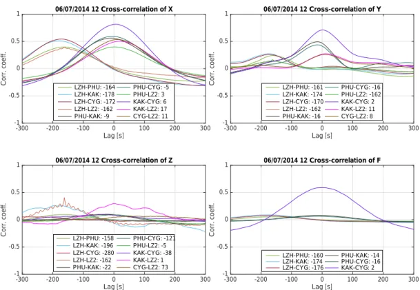
To obtain the estimation of the time lag, the filtered time series of each measured component at all observatories have been cross-correlated in pairs. An example for that same day, during local night, is shown in Fig. 2. The cross-correlation with the second acquisition system available at Lanzhou is
also shown in this figure. The cross-correlation curves show that it is easier to estimate the lags between time series using the X and Z components, because they present quite sharp peaks. Observatories with reliable time stamp show a cross-correlation lag near to 0 s, but it can sometimes exceed 10 s, if the cross-correlation peak is wide. Data from all observa-tories correlated with LZH time series agree to estimate the lag between 162 and 196 s.
From this first analysis, it appeared clearly possible to use distant observatories for verifying the data synchronization, but the precision is not sufficient for the purpose of correcting the data time stamps. We computed estimates of the time lag for each day between January 2013 and July 2014, obtaining
314 P. Coïsson et al.: Time-stamp correction of observatory data -300 -200 -100 0 100 200 300 Lag [s] -1 -0.5 0 0.5 1 Corr. coeff. 06/07/2014 12 Cross-correlation of X LZH-PHU: -164 LZH-KAK: -178 LZH-CYG: -172 LZH-LZ2: -162 PHU-KAK: -9 PHU-CYG: -5 PHU-LZ2: 3 KAK-CYG: 6 KAK-LZ2: 17 CYG-LZ2: 11 -300 -200 -100 0 100 200 300 Lag [s] -1 -0.5 0 0.5 1 Corr. coeff. 06/07/2014 12 Cross-correlation of Y LZH-PHU: -161 LZH-KAK: -174 LZH-CYG: -170 LZH-LZ2: -162 PHU-KAK: -16 PHU-CYG: -16 PHU-LZ2: -162 KAK-CYG: 2 KAK-LZ2: 11 CYG-LZ2: 8 -300 -200 -100 0 100 200 300 Lag [s] -1 -0.5 0 0.5 1 Corr. coeff. 06/07/2014 12 Cross-correlation of Z LZH-PHU: -158 LZH-KAK: -196 LZH-CYG: -280 LZH-LZ2: -162 PHU-KAK: -22 PHU-CYG: -121 PHU-LZ2: -5 KAK-CYG: -38 KAK-LZ2: 1 CYG-LZ2: 73 -300 -200 -100 0 100 200 300 Lag [s] -1 -0.5 0 0.5 1 Corr. coeff. 06/07/2014 12 Cross-correlation of F LZH-PHU: -160 LZH-KAK: -174 LZH-CYG: -176 PHU-KAK: -14 PHU-CYG: -16 KAK-CYG: 2
Figure 2. Cross-correlation between all analysed observatories over 1 h of data (11:30–12:30 UTC) on 6 July 2014, one of the last days without GPS synchronization for LZH data logger. The second acquisition system of Lanzhou observatory is labelled LZ2.
coherent trends for all pairs of observatories. Figure 3 shows the time lags obtained using Kakioka observatory data for each measured component. The time lag estimation is very noisy on Z and Y components and the lower sampling of F at Lanzhou produces a curve that is more spread than for the X component. Nevertheless, the variation of the time lag during the year is evident. Changing UTC of analysis or the length of the cross-correlation time window strongly affects the spreading of the resulting lags. The hours around noon are the ones where the lags are obtained with lower noise on the X component. During the period between 1 January and 7 March 2013, when the GPS synchronization of LZH observatory was still operational, the cross-correlation of 1 h X values around 05:30 UTC resulted in an average time lag of −3 s with a standard deviation of 11 s. A full set of figures and tables of statistical values for lags computed at each UTC is provided in the Supplement. The analysis of the evolution of the lags through the whole period reveals that two differ-ent trends are observed: a slow variation during 2013 and up to April 2014 and fast variations from April to July 2014, af-ter the data logger was rebooted and the correction for the oscillator frequency was lost.
It was therefore decided to use the data of the second ac-quisition system available in Lanzhou inside the same build-ing for computbuild-ing the time lags suitable for correctbuild-ing the time stamps. Two different sensors were deployed on the second acquisition system, one in 2013 and another in 2014,
making it possible to generate a complete dataset for compar-ison. The resulting curves, shown in Fig. 4, present coherent lag values for all the three components X, Y , Z, and the F component is more noisy due to the lower sampling rate of the scalar magnetometer. In particular, the Z component ex-hibits a very small dispersion of data and just a few outliers: it is the component where the amplitude of the spikes occur-ring in this observatory is larger. These short spikes, lasting 3 to 5 s, are local phenomena that can be used to precisely estimate the lag between the two time series since they pro-duce a very narrow peak in the cross-correlation curve (see Fig. 2).
2.2.1 Correction of data time stamp
After computing all the time lags, it was decided that only the period up to 2 April 2014 was suitable for time-stamp correction, since the clock drift was very slow during that time. Data for the period between 2 April and 8 July 2014, when the time drift was of 2 s per day, will not be pub-lished as definitive data. A new set of corrected LZH 1 s data files was then generated using the computed time lags based on the second instrument available in Lanzhou ob-servatory. A single daily correction value was used since the lags were nearly constant during 1 day. This correction value was calculated for 12:00 UT, following a smooth hy-perbolic tangent function fitted to the calculated delays. This choice was possible since the drift of the clock was always
j f m a m j j a s o n d j f m a m j j a Month -180 -150 -120 -90 -60 -30 0 30 60 90 120 150 180 lag [s] j f m a m j j a s o n d j f m a m j j a Month -180 -150 -120 -90 -60 -30 0 30 60 90 120 150 180 lag [s] j f m a m j j a s o n d j f m a m j j a Month -180 -150 -120 -90 -60 -30 0 30 60 90 120 150 180 lag [s] j f m a m j j a s o n d j f m a m j j a Month -180 -150 -120 -90 -60 -30 0 30 60 90 120 150 180 lag [s] 0 5 10 15 20 UTC [h] Lanzhou - Kakioka 2013 2014 2013 2014 2013 2014 2013 2014
Figure 3. Time lags calculated every day during 1 h around 17:30 UTC comparing Lanzhou and Kakioka data for each component of the magnetic field X, Y, Z and F . The F component is measured every 5 s at Lanzhou. The vertical lines indicate from left to right: the time when the GPS synchronization became unavailable, the time when the data logger was rebooted and the time when the GPS synchronization was re-established.
well below the 5 s month−1recommended by INTERMAG-NET (INTERMAGINTERMAG-NET Operations Committee and Execu-tive Council, 2012) for computing 1 min values. The cor-rected 1 s data files were averaged to compute 1 min data files following the INTERMAGNET recommendations for data filtering (INTERMAGNET Operations Committee and Executive Council, 2012). Lastly, the baseline processing al-lowed to generate corrected 1 min definitive data for LZH observatory.
3 Discussion
The time synchronization of LZH VM391 and GSM90 in-struments was lost on 7 March 2013, but it was noticed only 1 year later since the drift of the data logger clock was very slow. At that time, the acquired data had accumulated a lag of 28 s compared to UTC time (Fig. 4). This drift is rela-tively low, thanks to the correction of the oscillator frequency that is done by the data logger. During the first 2 months, only 2 s of lag were accumulated. In the period between June and September the lag increased at a faster rate and reached 24 s. Afterwards the lag increased more slowly, to reach a sta-ble level of 27 s in December 2013. It remained at this level
up to mid-March 2014, when a slow increase started again. 28 s lag was reached just before the data logger reboot on 2 April 2014.
The most significant part of the lag was accumulated dur-ing the summer months, when the temperature of the data logger was the highest (Fig. 5). The automatic monitoring of the LZH acquisition system include measurements of the temperature of some components, but not the oscillator tem-perature. The closest available temperature is the one of the energy card and we analysed its evolution to understand if it could reveal useful information to interpret the variation of the time lag. Though a correlation between the quartz fre-quency and the temperature of the data logger is expected, it might be non-linear. The temperature of the energy card follows a seasonal trend. It appears that the difference be-tween this temperature and its value at the time when Fcounter was last estimated played an important role in the clock drift. Only when this temperature difference was exceeding 5◦C did the clock drift at a higher pace. When the temperature returned below this 5◦C difference, the clock nearly stopped drifting. At the reboot of the data logger on 2 April 2014, the clock correction parameters were erased from its mem-ory and were no longer available. It was not possible for the data logger to compute a new correction, since the PPS was
316 P. Coïsson et al.: Time-stamp correction of observatory data j f m a m j j a s o n d j f m a m j j a Month -180 -150 -120 -90 -60 -30 0 30 60 90 120 150 180 lag [s] j f m a m j j a s o n d j f m a m j j a Month -180 -150 -120 -90 -60 -30 0 30 60 90 120 150 180 lag [s] j f m a m j j a s o n d j f m a m j j a Month -180 -150 -120 -90 -60 -30 0 30 60 90 120 150 180 lag [s] j f m a m j j a s o n d j f m a m j j a Month -180 -150 -120 -90 -60 -30 0 30 60 90 120 150 180 lag [s] 0 5 10 15 20 UTC [h] Lanzhou - Lanzhou2 2013 2014 2013 2014 2013 2014 2013 2014
Figure 4. Time lags calculated for every hour using the data of the two acquisition systems available at Lanzhou observatory for each component of the magnetic field X, Y, Z and F . The F component is measured every 5 s at Lanzhou; the second scalar magnetometer was not available in 2014. The vertical lines indicate from left to right: the time when the GPS synchronization became unavailable, the time when the data logger was rebooted and the time when the GPS synchronization was re-established.
35 30 0 2...25 20 15 10�--�--�---�--�--��--�� 01/13 04/13 07/13 10/13 01/14 04/14 07/14 Date [month/year]
Figure 5. Seasonal variation of the data logger energy card temper-ature during 2013 and 2014. This tempertemper-ature is measured every minute and we assumed that it is similar to the oscillator tempera-ture.
not in operation due to the GPS failure. The data logger clock started drifting with a constant rate of about 2 s per day. Ad-ditional reboots were done afterwards, and at every reboot the clock counter started at a different value producing the saw-tooth behaviour that can be observed in the lags shown in Fig. 4.
To avoid having similar issues in the future, some options are possible:
– Use a data logger with a temperature-compensated crys-tal oscillator (TCXO).
– Improve the software for clock correction to save the corrections to the quartz frequency so that they are avail-able even after a reboot of the data logger and possibly also include temperature correction.
– Improve the monitoring tools of the observatory so that similar failures could be detected more easily. It should be pointed out that this particular situation occurred be-cause, at that time, the log files were not routinely trans-mitted along with the data files.
LZH monitoring data are now regularly transmitted to IPGP and checked to prevent future occurrences of unnoticed time synchronization unavailability.
4 Conclusions
The GPS time synchronization of LZH magnetic observa-tory was lost on 7 March 2013. Over 1 year, the time-stamp attribute to the acquired data had accumulated a lag of 28 s compared to UTC time. This drift is low, thanks to the correc-tion of the oscillator frequency that is done by the data logger. It is possible to confidently correct the time stamps of the 1 s acquisitions to produce 1 min definitive data, the official IN-TERMAGNET products. It has been proven by comparing the time series of one observatory at mid-latitude with the time series of observatories within 3500 km range that it is possible to detect the correct trend of time drift. This compar-ison is more effective during hours when there is low diurnal variation and is better identified on the magnetic X compo-nent. This is an effective way to verify the stability of clocks in un-manned acquisition systems that cannot be monitored in real time. To be able to construct a precise time correction function it is preferable to use another acquisition system lo-cated in the same premises, like in Lanzhou observatory. In this case, all spikes caused by local activities, that are usually removed from magnetic definitive data, provide short signals that facilitate obtaining a precise time correction. In the case of Lanzhou, the vertical component of the magnetic field is the one most affected by spikes and could be used to correct the synchronization of the time series. The time stamps for the whole period between March 2013 and 8 April 2014 were corrected and averaged 1 min values definitive data could be produced.
Data availability. Magnetic observatory data used for this pa-per are available at the Bureau Central de Magnetisme Terrestre (BCMT) website (www.bcmt.fr) or on BCMT – Magnetic data-bank https://doi.org/10.18715/BCMT.MAG.DEF and on INTER-MAGNET website (www.intermagnet.org). Definitive 1 min data of LZH observatory will also be included in INTERMAGNET annual DVDs, available upon request at intermagnet@ipgp.fr.
The Supplement related to this article is available online at https://doi.org/10.5194/gi-6-311-2017-supplement.
Author contributions. PC analysed the data, produced the corrected files and wrote the article; BH identified the problem and produced definitive data; KT and XL developed the LZH observatory acqui-sition system and interpreted the instrument response; VL validated the methodology; and CJX processed the data. PC prepared the pa-per with contributions from all co-authors.
Competing interests. The authors declare that they have no conflict of interest.
Special issue statement. This article is part of the special issue “The Earth’s magnetic field: measurements, data, and applications from ground observations (ANGEO/GI inter-journal SI)”. It is a re-sult of the XVIIth IAGA Workshop on Geomagnetic Observatory Instruments, Data Acquisition and Processing, Dourbes, Belgium, 4–10 September 2016.
Acknowledgements. The results presented in this paper rely on the data collected at Lanzhou, Phu Thuy, Da Lat, Kakioka and Cheongyang observatories. We thank IPGP, Chinese Earthquake Administration, Vietnam Academy of Science and Technology, Japan Meteorological Agency, Korea Meteorological Admin-istration for supporting their operations and INTERMAGNET for promoting high standards of magnetic observatory practice (www.intermagnet.org). We thank the two anonymous reviewers for their constructive comments that allowed improving the article. This is IPGP contribution 3854.
Edited by: Christopher Turbitt Reviewed by: two anonymous referees
References
Changjiang, X. and Zhang, S.: The Analysis of Baselines for Different Fluxgate Theodolites of Geomagnetic Ob-servatories, Data Science Journal, 10, IAGA159–IAGA168, https://doi.org/10.2481/dsj.IAGA-23, 2011.
Chulliat, A., Savary, J., Telali, K., and Lalanne, X.: Acquisition of 1-second data in IPGP magnetic observatories, in: Proceedings of the XIIIth IAGA Workshop on Geomagnetic Observatory In-struments, Data Acquisition, and Processing, edited by: Love, J. J., Open-File Report 2009–1226, 54–59, U.S. Geological Survey, 54–59, available at: https://pubs.er.usgs.gov/publication/ ofr20091226 (last access: 9 August 2017), 2009.
INTERMAGNET Operations Committee and Executive Coun-cil: INTERMAGNET Technical Reference Manual, 4.6th Edn., available at: http://www.intermagnet.org/publication-software/ technicalsoft-eng.php (last access: 9 August 2017), 2012. Love, J. J. and Chulliat, A.: An International Network of Magnetic
Observatories, Eos, Transactions American Geophysical Union, 94, 373–374, https://doi.org/10.1002/2013EO420001, 2013. Peltier, A. and Chulliat, A.: On the feasibility of promptly producing
quasi-definitive magnetic observatory data, Earth Planets Space, 62, e5–e8, https://doi.org/10.5047/eps.2010.02.002, 2010. Thebault, E., Finlay, C., Beggan, C., Alken, P., Aubert, J.,
Bar-rois, O., Bertrand, F., Bondar, T., Boness, A., Brocco, L., Canet, E., Chambodut, A., Chulliat, A., Coïsson, P., Civet, F., Du, A., Fournier, A., Fratter, I., Gillet, N., Hamilton, B., Hamoudi, M., Hulot, G., Jager, T., Korte, M., Kuang, W., Lalanne, X., Langlais, B., Leger, J.-M., Lesur, V., and Lowes, F.: International Geomag-netic Reference Field: the 12th generation, Earth Planets Space, 67, 79, https://doi.org/10.1186/s40623-015-0228-9, 2015. Yang, D.: Observatories in China, in: Encyclopedia of
Geo-magnetism and PaleoGeo-magnetism, edited by: Gubbins, D. and Herrero-Bervera, E., Springer Netherlands, Dordrecht, 727–728, https://doi.org/10.1007/978-1-4020-4423-6_235, 2007.