HAL Id: hal-02268106
https://hal.umontpellier.fr/hal-02268106
Submitted on 14 Oct 2019
HAL is a multi-disciplinary open access
archive for the deposit and dissemination of
sci-entific research documents, whether they are
pub-lished or not. The documents may come from
teaching and research institutions in France or
abroad, or from public or private research centers.
L’archive ouverte pluridisciplinaire HAL, est
destinée au dépôt et à la diffusion de documents
scientifiques de niveau recherche, publiés ou non,
émanant des établissements d’enseignement et de
recherche français ou étrangers, des laboratoires
publics ou privés.
Towards robust scenarios of spatio-temporal renewable
energy planning: A GIS-RO approach
Nadeem Al-Kurdi, Benjamin Pillot, Carmen Gervet, Laurent Linguet
To cite this version:
Nadeem Al-Kurdi, Benjamin Pillot, Carmen Gervet, Laurent Linguet. Towards robust scenarios of
spatio-temporal renewable energy planning: A GIS-RO approach. 25th International Conference on
Principles and Practice of Constraint Programming, Sep 2019, Stamford, United States. �hal-02268106�
renewable energy planning: A GIS-RO approach
Nadeem Al-Kurdi1, Benjamin Pillot1, Carmen Gervet2, and Laurent Linguet11
ESPACE-DEV, Univ Guyane, Univ Montpellier, IRD, 275 route de Montabo, BP
165 - 97323 Cayenne Cedex, Guyane Fran¸caise
2
ESPACE DEV, Univ Montpellier, Univ Guyane, IRD, 500 rue Jean Fran¸cois
Breton, 34090 Montpellier, France
Abstract. Solar-based energy is an intermittent power resource whose potential pattern varies in space and time. Planning the penetration of such resource into a regional power network is a strategic problem that requires both to locate and bound candidate parcels subject to multiple geographical restrictions and to determine the subset of these and their size so that the solar energy production is maximized and the associated costs minimized. The problem is also permeated with uncertainty present in the estimated forecast energy demand, resource potential and technical costs. This paper presents a novel combination of Geographic Information Systems (GIS) and Robust Optimization (RO) to develop strategic planning scenarios of a collection of parcels that accounts for their spatio-temporal characteristics, and specifically their hourly radiation patterns that are location dependent, to best fit the network temporal demand and minimize technical costs.
The problem is formulated as a GIS spatial placement problem and a RO fractional knapsack problem to plan the effective power penetration and geographical suitability of new PV facilities. The combination GIS-RO generates an excellent decision support system that allows for the computation of optimized parcel scenarios (locations, sizes and power). The qualitative and quantitative effectiveness of the approach is demon-strated on real data on the French Guiana region. Results show that the proposed approach provides reliable fine grained planning that also accounts for the risk adversity of the decision maker towards forecast demand and solar potentials.
Keywords: Renewable energy planning · Geographic Information sys-tems · Robust optimization.
1
Introduction and related work
Energy transition from a high-carbon regime born of fossil fuels to low-carbon solutions is a major challenge of current societies [10]. Most of the energy plan-ning strategies therefore aim at enhancing the share of renewable energy (RE) sources within power networks [23]. When those energies are dispatchable, the integration remains pretty straightforward [16,36]. However, when it comes to
volatile, or intermittent RE sources, this is no longer true. Their unstable and variability nature implies that the resulting aggregated power injected into the grid may threaten network’s stability by not matching the power demand [23].
Thus, the full problem of integrating intermittent RE sources in power net-works involves irregular spatio-temporal energy potential patterns, related to the location and dimensions of power facilities. It is a multi-criteria uncertain optimization and planning problem that combines the spatial placement of can-didate parcels for installing power facilities subject to geographical constraints and temporal resource constraints, and the selection (location, size and capacity) of optimal plants such that the power into the network is increased at minimal costs and short-term unpredictability is limited to an acceptable level.
Taking into account spatio-temporal energy potential data, together with heterogeneous land, network, and technico-economic constraints for effective re-newable energy planning remains a challenging multi-dimensional problem per-meated with uncertain data [37]. The computational approaches are broadly di-vided into two research streams: 1) geographical information system (GIS) mod-eling with multi-criteria decision-making (MCDM) [6,13,34,3], and 2) bottom-up engineering approaches [23,35,7,37]. GIS models with MCDM focus on providing suitability maps based on static resource assessment and expert-based decision criteria. The maps depict areas with their respective weighted criteria values to be used in the MCDM model, such as economic, environmental or techni-cal ones. These approaches do not aim at optimizing the actual parcel selection that would require taking into consideration the short-term temporal variation of both the resource and power demand, or their evolution in the long-term. On the other hand, bottom-up engineering approaches allow for time simulation and optimization of given energy system configurations. Their main objective is to guide energy policy road map often at a national scale and longer time horizon. This systemic approach gives a significant insight into the potential contribution of RE sources [12,11], but does not aim at identifying physical par-cel locations. Similarly [22] addresses the resource management problem as a knapsack problem, that shows the suitability of linear programming to select among experts’ given parcels, the ones with highest resource potential. It does not consider the hourly temporal patterns of the different sites and their pro-jected uncertainty, the possibility to consider a fraction of a given parcel, nor the impact of geographical restrictions and distances, and the complexity of the associated technical costs.
In summary, to date we are not aware of computational approaches that tackle the spatio-temporal optimization problem consisting of identifying the best parcels that increase solar energy penetration into the network at minimal cost, while satisfying a region’s specific constraints (terrain, resource, infrastruc-tures, etc) and related costs. This paper addresses this problem by proposing a two-steps specification in terms of a spatial placement and a resource planning problem, and we propose an integrated computational approach. The approach contributes a novel framework based on GIS spatio-temporal data and constraint processing, connected to a Robust Optimization (RO) knapsack model to plan
renewable energy scenarios. The combination GIS-RO generates an excellent de-cision support system that allows for the planning of parcel scenarios (locations and areas) that will best increase the RE power into the network at minimal cost, according to the decision maker risk adversity. A GIS can handle very large volumes of data, including remote sensing images for solar radiation in-dicators, land use maps, and various networks maps (electrical, roads, water). The application of global and multi-layers geographical constraints and various control parameters allow for an effective deterministic pruning of the region, to determine suitable candidate parcels, and their relevant properties without impairing the optimization problem.
The core contributions of this paper are: 1) the specification of a complex spatial placement and planning problem, 2) a computational approach that ef-ficiently exploits GIS geographical constraints, and makes powerful use of large scale spatio-temporal environmental data, and 3) an integration of the spatial analysis with a robust optimization module through a comprehensive set of re-source and contextual features. Through the use of Robust Optimization, data uncertainty present in the forecast figures for the planned horizon is tackled with a measure of robustness, allowing best and worst case scenarios to be studied according to various risk adversity positions of the decision maker.
The GIS-RO framework presented in this paper, is applied to a real world challenge of PV solar power plants planning in the region of French Guiana. It illustrates the qualitative and quantitative efficiency of the approach as a decision support system providing solution scenarios. The paper is organized as follows: Section 2 describes the problem and overall approach; section 3 presents the GIS module; section 4 the robust optimization model; section 5 is the experimental section based on a real-world case study for robust spatial decision making from time series resources; and section 6 concludes the paper.
2
Problem description, application and approach
The problem is motivated by a renewable energy scenario planning problem from the 2015 Energy Transition Act. France’s energy policy has the target for overseas regions, in particular French Guiana, of 50 % of renewable energy in final consumption in 2020 and full energy self-sufficiency by 2030 [15]. The chal-lenge is to identify suitable candidate parcels for RE parks and determine the ones, and their optimal size, that would maximize power network contribution at minimal costs. A candidate parcel must satisfy a number of geographical con-straints, including topographic land use restrictions, type of ground surface, be at a maximum distance threshold from the electrical grid, and have a maximum surface with limited land slope. These constraints bound the areas for candidate parcels.
The scenarios for the best parcels selection deal with the resource potential and costs associated with each candidate parcel. The intermittent resource fol-lows a temporal pattern specific to the geographic location. The costs are mainly technical costs (installation, maintenance, grid connection) that depend on the size of the parcel and its distance to the grid. These data have a degree of
un-certainty in terms of their future value. The full problem can actually be defined as a spatial placement problem to identify candidate parcels, and a fractional uncertain knapsack problem with forecast time-series resource, to compute sce-narios of optimal parcel selection and sizes. This paper aims at defining and showing the strengths of a combined GIS and RO computational approach to tackle complex spatial decision making problems with time-series resources, with application here to solar energy placement and planning.
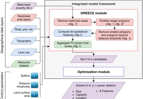
Integrated computational work-flow The work-flow depicted in Fig. 1 best de-scribes the computational process and integration of the two modules. We first describe the main inputs, then each module. Geographical data layers and con-trol parameters input the developed GIS GREECE module, which implements methods to determine the candidate parcels, and contributes a despatialization of the relevant features for each parcel (resource pattern, maximal size and costs), needed to enrich the RO model.
Fig. 1: GIS-RO integrated workflow
Data, constraints and control parameters In GIS terminology, the concept of layer corresponds to geographic datasets. When the dataset is an image, the term Raster is commonly used. The geometric objects are in vector mode and can be specified as polygons, lines or points. As depicted in Fig. 1, input data layers correspond to: 1) the study region or base layer, 2) the restricted area layers, 3) specific objects for which distance to resulting polygons must be computed (e.g. road, grid), 4) terrain features (land use and topography) and 5) the resource of interest (here solar radiation maps).
The restricted area layers stand for polygons where facilities cannot or should not be established. Typically, they include urban areas, ecological zones,
water-courses, military sectors, cultural heritage, etc. They may also represent zones too far from specific objects (e.g. electrical grid). Geographic elements for which distance must be computed can be of any kind but are generally related to con-nection and accessibility costs such as road and grid networks. Topography and land use allow terrain to be characterized within each polygon. Finally, resource dataset is a set of raster or vector processed images, potentially with time series. Data layers and maps are retrieved from national and international geographic databases or remote sensing image processing.
The range control parameters are set by the user, and allow for different land management scenarios to be generated. Buffers surrounding geographic objects depend both on their type and on the kind of power station. Distance thresholds to given layers (e.g. road network, electrical grid) stand for the limit beyond which establishing a facility is not economically viable. Finally, land surface area specify a region’s land management in terms of minimum and maximum allowed surface thresholds. Smaller or larger parcels might respectively be excluded from the study, or partitioned into suitable smaller parcels.
3
GIS module: GREECE
We specify the Geographical REnewable Energy Candidate Extraction problem below, then describe our spatial partitioning and placement solution methods.
Given:
Blayer Base layer (i.e. a set of polygons)
Rlayer Restricted area layers
Dlayer Distance threshold layers (i.e. sets of geometries)
h Matrix of elevation values (DEM) associated to the base layer
Rmaps Set of resource raster maps
LUlayer Land-use layer
N ETlayers Layers (e.g. grid, roads, ...) for which distance to each resulting
polygon must be calculated
Buf f ers Control parameter: Set of buffer values, each associated with a given layer
DistT Control parameter: Set of distance threshold values, defined for each Dlayer
smin, smaxControl parameter: Surface thresholds
Find:
The set P of candidate parcels
The de-spatialized resource time series and geographical features for each parcel Such that the following geographical restrictions hold:
A candidate parcel is geographically disjoint from all layers of restricted areas The surface of a candidate parcel is within given bounds
A candidate parcel is within a bounded distance from the threshold layers
For space reasons, we give the main procedure in Algorithm 1, the spatial partitioning algorithm, and describe our spatial slicing and extraction methods, developed with Python GIS packages. The general procedure is decomposed in two main steps: 1) spatial placement and partitioning (Alg.1: line 2-10) , 2) conversion of the resulting polygons defined by their geographical coordinates into de-spatialized items with relevant features (Alg.1: line 11-20). The set of
relevant built-in Python GIS functions for topological, raster, set and graph operations is defined (packages used:geopandas,shapely,rtree,gdal[21],numpy
[43], and networkx).
Topological geometric and raster images operators
DISTANCE(p,P ) Minimum euclidean distance between centroid
of polygon p and all elements in set P
UNION(p1, .., pn) geometric union of the polygons pi
RTREEIDX(P ) Compute spatial index idx of all elements in P
INTERSECTS(p,P,idx ) geometric intersection of p with elements in P
SHAPE(p) Shape factor of polygon p (e.g. roundness)
SURFACE(p) Surface of polygon p
SLOPE(h) Slope raster from the Digital Elevation Model h
ASPECT(h) Raster of slope orientation values from DEM h
Set and graph functions
HONEYCOMB(x,shex) Creates a honeycomb grid corresponding to polygon x
of x with hexagonal elements having surface shex
PARTGRAPH(G, n, Wpart) Partitions a graph G into n parts having weights Wpart
Algorithm 1: GREECE main algorithm
1 begin
2 /* Compute candidate parcels specified spatially as polygons */
3 P ← MASK(Blayer, Rlayers, Buf f ers)
4 for p ∈ P :
5 if SURFACE(p) >= smax:
6 P .DELETE(p)
7 P .INSERT(PARTITION(p, smax, fd))/* see algorithm 2 */
8 for p ∈ P :
9 if SURFACE(p) < smin∨ DISTANCE(p, i ∈ Dlayer) > dti, dti∈ DistT :
10 P .DELETE(p)
11 /* Compute, store de-spatialized features for each polygon p
(Section 3.2) */
12 for p ∈ P :
13 p.APPEND(DISTANCE(p, N ∈ N ETlayers))
14 p.APPEND(SHAPE(p)), p.APPEND(SURFACE(p))
15 p.APPEND(sk∈ SURFACE(p ∩ INTERSECTS(p, LUlayer,
RTREEIDX(LUlayer))))
16 /* Aggregate raster cell values, terrain features, within p */
17 p.APPEND(µn∈ ZONALSTAT({h, SLOPE(h), ASPECT(h)}, p, µ))
18 p.APPEND(σn∈ ZONALSTAT({h, SLOPE(h), ASPECT(h)}, p, σ))
19 /* Mean energy resource values per raster time series */
20 p.APPEND({µ1, µ2, · · · , µt} ∈ ZONALSTAT(Rmaps, p, µ))
3.1 Spatial placement and partitioning of polygons
Slicing the base layer: extracting parcel polygons The slicing of the whole study area is divided into two main steps. The first consists in identifying and removing
the restricted areas that intersect a base polygon (our study area) as well as zones beyond the distance threshold from given elements (electrical grid, road network, etc.). The procedure MASK(Blayer, Rlayers, Buf f ers) applies set-based
topological operators, that mask out portions of restricted layers and buffered zones, intersecting the base layer (Alg.1:line 3). It corresponds to a 2-dimensional difference operation. The result of this first step is a finite set P of new polygons, representing available land for potential power facilities, illustrated in Fig 2 (a). The second step (Alg.1:lines 4-10), consists in filtering in a deterministic manner the polygons belonging to this set, based on their surface and distance to the grid. First we identify the parcels whose surface is beyond the allowed threshold. We developed a 2D space partitioning approach based on a k-way graph partitioning method, that partitions these parcels into smaller ones of suitable sizes (Algorithm 1: line7). Then, we prune further the resulting set of potential parcels according to the minimal surface threshold and distance to the grid, illustrated in Fig 2 (b). This last step is best handled using GIS geographical metric operators (Alg.1: lines 8-10). The extracted and computed parcels can all contribute to a solution, without inconsistent pruning of viable parcels from the standpoint of the threshold and land restriction constraints. Fig.2 illustrates the spatial layers masking process as well as the pruning of parcels below a surface threshold, and beyond a distance threshold to network layers (grid, roads, ...).
p m1
m2
m3
p*
(a) Masking process
layer P layer Di
DISTANCE(p, Di) > dmax
SURFACE(p) < smin
(b) Distance, area threshold constraint processing
Fig. 2: Pruning restricted areas and threshold layers
Spatial partitioning method To partition a polygon into smaller plots of equal size, we propose a k-way graph partitioning approach, depicted in Alg. 2. First, we specify the initial polygon as a honeycomb mesh, that is a set of connected hexagonal plots of given size (line 6). We then map the mesh to a graph, and apply a k-way graph partitioning (lines 7, 20-29). Each hexagon denotes a vertex connected to its concomitant neighbors by unweighted and undirected edges. The k value is first initialized using a desaggregation factor, that sets the size of each hexagon (lines 3-5). The bigger the factor value, the smaller each hexagon and thus the more refined is the mesh. Each vertex is weighted with the correspond-ing hexagon surface. The weight of the sought clusters (final plots) is initialized (lines 8-13), to feed the k-way graph partitioning (line 15). The procedure derives k clusters of vertices, to reach the surface threshold of each plot. The algorithm minimizes the number of edge cuts and forces contiguous partitions [29], so that
Algorithm 2: Surface partitioning
1 def PARTITION(p, smax, fd): /* Partition polygon p into a set of
polygons P of equal surface */
Input : polygon p, maximal area per partition smax, disaggregation
factor fd
Output : a set P of polygons
2 /* Initialization */
3 k ← bSURFACE(p)
smax c /* Number of targeted plots */
4 if k <= 1 and SURFACE(p) − spart< spart/fd:
5 return {p}
6 H ← HONEYCOMB(p, area:smax/fd) /* create the mesh of hexagons */
7 G ← TOGRAPH(H, SURFACE(hexa ∈ H))
8 for i ∈ {1, .., k}:
9 /* Set the weight for each sought plot */
10 Wplot.APPEND(smax)
11 if SURFACE(p) mod smaxnot = 0:
12 Wplot.APPEND(SURFACE(p) − n · smax)
13 k ← k + 1
14 /* k-way graph partitioning of G into a set of k clusters C */
15 C ← PARTGRAPH(G, k, Wplot)
16 /* Convert the clusters of vertices into a set polygons */
17 for set ∈ C:
18 P .INSERT(UNION(pi| i ∈ set))
19 return P
20 def TOGRAPH(H, Whexa): /* Convert the weighted mesh into a graph */
Input : set of hexagons H, set of corresponding weights Whexa
Output : a graph G
21 /* Initialization */
22 G ← GRAPH()
23 for (h, w) ∈ (H, Whexa):
24 /* set of polygons concomitant to h, frontiers */
25 F ← INTERSECTS(h, H, RTREEIDX(H))
26 for f ∈ F :
27 G.INSERT(EDGE(h, f ))
28 G.INSERT(NODE(p, weight:w))
29 return G
the final aggregates present round-like geometries. The algorithm was devel-oped using Python library networkx and the METIS package [30]. Finally the k-clusters are translated into k polygons (lines 17-18).
Example 1. The figure illustrate a 16-way graph partitioning of a 781 km2
poly-gon into plots of 50 km2, using an hexagonal honeycomb mesh. k is initialized
to b78150c. The algorithm derives 15 plots between 49 km2 and 51 km2 plus one
is a finite set of polygons of acceptable surface (below the maximum threshold).
*
1 1 1 1 1 1 1 1 1 1 1 1 1 1 1 1 1 1 1 1 2 2 2 2 2 2 2 2 2 2 2 2 2 2 2 2 2 2 2 2 2 2 2 2 3 3 3 3 3 3 3 3 3 3 3 3 3 3 3 3 3 3 3 33.2 Contextual data and resource time series de-spatialization Geospatial data is an invaluable source of contextual information, to charac-terize in general, multiple land features and resources, but also their proximity with all sorts of infrastructure networks. The challenge when dealing with opti-mization problems evolving around resources, costs and constraints, is to seek a computational approach to specify and solve a problem as closely as possible to its real setting. A contribution of the proposed GIS-RO framework is to achieve this by using the qualitative and large spatio-temporal and contextual informa-tion analyzed and extracted through GREECE, with a de-spatilizainforma-tion process. The goal is to convert the polygons into items without their geo-referencing, and to associate to each the features relevant to the optimization module. Re-garding energy planning, the features must capture many land properties, and resource time series, but also dimensions and distances that will allow a reliable conversion to technical costs for each candidate parcel.
The localization and maximal surface of a candidate parcel can provide nu-merous relevant information from the intersected data layers: 1) the distance to specific infrastructures such as substations, electrical grid or road network contributes to assessing energy losses as well as accessibility costs, 2) the maxi-mal surface is linked to construction and maintenance costs [42,6,3]. In addition, terrain slope is a critical criterion for establishing power facilities [4,46]; in the same way, final cost might also be affected by land type and land use, or even the shape of the parcel. In the case of solar and wind energies, geo-referenced resource maps are available from satellite images or field studies [20,5,6]. By overlaying the previously sliced polygons with these raster images, it is therefore possible to aggregate the resource within each parcel. Essentially, the de-spatialization consists in translating the geography of each candidate into either static or dy-namic quantifiable features. These features can then be integrated into energy models, converted into construction and operation costs, or used as constraints or in the objective functions of the optimization model. In the case of solar PV, GREECE extracts the following parameters from each candidate parcel: area, shape, distance to the grid, land use share, elevation, slope, aspect and solar GHI time series (Alg. 1:lines 13-20). The whole implementation has made use of the python libraries referred earlier. SURFACE(p) provides information on the maximum power plant capacity that could eventually be set up within the par-cel. SHAPE ranges from 0 to 1 and measures the roundness of a parcel, that is
how spread out a solar PV plant might eventually be. DISTANCE to the grid is computed from the polygon centroid and is used to get both connection costs and transmission losses. Land use share can be correlated to construction costs, as well as elevation (from DEM h) using SLOPE and ASPECT. They may also be used as exclusion thresholds. Land use share is retrieved by computing the intersecting area between the given parcel and each attribute of a land use layer LUlayer (line 15). Elevation, slope and aspect are retrieved from the 3 arc
sec-ond SRTM-based digital elevation model (DEM) [27] and by calculating average and standard deviation from raster cells overlapping with each candidate parcel (lines 17-18). Finally, solar GHI time series are obtained in the same way as with the DEM but for as many time steps as available solar radiation maps (line 20). As a result, each candidate parcel is now a compound item with geometric and terrain features, and time series of solar GHI values. In the case of solar PV, we have also converted GHI into power by adapting thepvlib library from the Sandia National Laboratory (SNL) [25].
4
Optimization module - fractional knapsack approach
The Optimal planning and sizing of PV plants (OPSPV) is an optimization problem permeated with uncertainty, rooted in projection estimates from cur-rent data relative to the growth of energy demand and the resource values. As shown in Fig. 1, it takes the candidate parcels with their de-spatialized features to select the ones and their optimal size such that the PV power penetration in the network is maximized at minimal cost. We propose a robust optimiza-tion approach based on the seminal works of [8,14], that specifies uncertainty using deterministic intervals. They denote the robust bounds within which the uncertain data is known to take its value. This modelling approach enables re-liable best and worst case planning scenarios to guide the decision makers, and to assess the impact of his risk adversity impact on the output scenarios. The specification of the problem is given in Fig. 3.
Robust constraint optimization model
The OPSPV, energy strategy planning problem can be modelled as a fractional knapsack problem with additional constraints. In this analogy, the knapsack corresponds to the forecast energy demand to be provided by existing and new intermittent RE sources (in KW/hr), and the items are the candidate parcels with their potential supply (KW/hr) plus their associated technical costs (in-stallation relative to the size thus production (e/KW ), and connection to the grid and substation (e). The objective is to maximize hourly penetration of additional RE power in the network while minimizing global costs.
We first specify the problem and then describe the model developed in terms of variables, constraints and cost functions.
Variables We consider two sets of variables that need to be linked to each other. Boolean variables relate to the selection or not of a candidate parcel, needed to determine whether the unit connection cost is applied or not (Cconi). The area
Given:
Unit: Hour (per year) t ∈ H = {1, · · · , 8760} Unit: Candidate parcel i ∈ N = {1, · · · , n}
Current hourly production from intermittent energy sources (KWh) Eintt
Current hourly production from non-intermittent energy sources (KWh) Ept
Estimated global hourly power demand (KWh) Demt= [Demt, Demt]
Nominal power of a PV unit (to convert plant size into power) P nom
Minimum and maximum area for each candidate parcel (m2) Smin, Smaxi
Estimated hourly production per PV unit (W h/m2) P pvt,i= [P pvt,i, P pvt,i]
Minimal distance from the grid to centroid of a candidate PV parcel (m) Dgi
Transmission line unit cost (e/m) Clan
Substation unit power cost (e/KW) Csta
Find:
The set of parcels where power stations will be built
The surface to consider for each candidate parcel that is selected Cost functions:
Sum of all costs of PV plant installation C = Σi(Ccapi+ Copi+ Cconi+ Cstai)
Unit capital cost for installing a PV power plant (e) Ccapi
Annual operational cost per new PV plant (e) Copi
Unit connection costs for each new PV plant, transmission lines (e) Cconi
Capital cost for new substation (e) Cstai
Total added PV energy production ΣtP Vt
Such that the following constraints hold:
PV newly added production plus existing production are below the hourly demand PV existing and new production are less than 35% of the total energy demand per hour PV parcel size cannot exceed a maximal set size
Fig. 3: OPSPV problem specification
constraint and the installation, capital and operational costs, that depend on the size of a new PV plant.
∀ i ∈ N, Bi∈ {0, 1} 1 if parcel is selected, 0 otherwise
∀ i ∈ N, SAi∈ [0.00..Smaxi] Area of a parcel
Knapsack constraints The first set of constraints relates to the forecast energy demand, using existing resources augmented with new PV production. It seeks to determine the capacity of new PV plants to contribute to the anticipated demand. Two scenarios are considered: 1) best case scenario (highest PV energy forecast and lowest forecast demand) and 2) worst case scenario (lowest PV energy forecast and highest forecast demand). This allows to study the impact of the decision maker risk adversity in planning the creation of new PV plants.
Best case scenario: ∀ t ∈ H, ΣiSAi× P pvt,i+ Eintt+ Ept≤ Demt
Worst case scenario: ∀ t ∈ H, Σi SAi× P pvt,i+ Eintt+ Ept≤ Demt
Network penetration constraints The second set of constraints states that the amount of intermittent energy resource into the network should be less than 35 % of the total forecast energy demand per hour (upper bound) [17]. The time stamp is the hour. It is also set for the best and worst case scenarios:
Best case scenario: ∀ t ∈ H, ΣiSAi× P pvt,i+ Eintt≤ 0.35 × Demt
Worst case scenario: ∀ t ∈ H, ΣiSAi× P pvt,i+ Eintt≤ 0.35 × Demt
Connecting parcel selection and size The third set of constraints establishes a link between the Boolean and PV plant area variables. This relationship is needed to connect the energy production and the various costs. If a plant size is not null then the parcel is selected, and conversely if a parcel is not selected its size is forced to be null.
∀i ∈ N, SAi≤ Smaxi× Bi, Bi× Smin ≤ SAi
Objectives and cost functions The OPSPV problem has two main objective functions: 1) to maximize the total hourly RE energy production over the year through new PV energy production, 2) to minimize the total technical costs. Since the functions are in different units, a single weighted function is not mean-ingful, instead we seek the pareto frontier, by optimizing PV production function while constraining the cost function with more restrictive values at each run. Maximize PV production: depending on the scenario considered, P pvt,i will
take its highest estimate (P pvt,i for best case) or lowest estimate (P pvt,i for the
worst case). The cost function to maximize is: ΣiΣtSAi× P pvt,i
Minimize costs: Modelling non-linear functions Four cost functions are involved and relate to the installation and size of a PV plant as defined in Fig. 3. Typi-cally, capital and operational costs are approximated as linear functions [9,24,19]. However, this approach is unrealistic as both the Capiand Copicosts are in fact
non-linear, since they depend on the size of the plant (linked to the related num-ber of PV panels) [31]. Basically the fewer the numnum-ber of panels the highest the relative cost per panel. To get closer to reality, we thus consider an innovative approach using a piece-wise linear function such that ai is the coefficient of the
slope, and yi the value of the coordinate where the new slope begins. It is
il-lustrated below for Capi, and Copi follows a similar specification with different
constants. Values have been set from [31]:
Capi= a1× P nom × SAi+ y1 if 0M W ≤ SAi× P nom ≤ 1M W a2× P nom × SAi+ y2 if 1M W ≤ SAi× P nom ≤ 10M W a3× P nom × SAi+ y3 if 10M W ≤ SAi× P nom
On the other hand, the unit connection cost of a PV plant, and the capital cost of a new station for a plant, are both linear functions that depend respec-tively on the creation of the plant in a parcel with its Euclidian distance to the grid, and the unit cost of a substation proportional to the computed size of the plant. We have the following functions:
5
Experimental study and evaluation
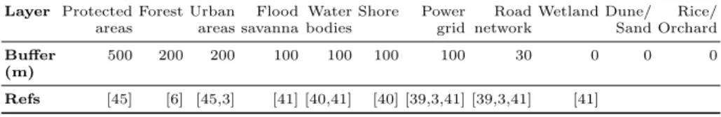
The proposed GIS-RO framework seeks to make powerful use of multi-scale con-textual information for spatial decision making and optimization. It is evaluated on the timely challenge in the region of French Guiana, where the objective is to reach the energy policy plan of 100% renewable by the year 2030, first by increasing PV, then biomass. The challenge lies in the strategic planning of solar PV scenarios using contextual real data characterized by spatio-temporal patterns and permeated with uncertainty (resource projections). In this section we present our results and analysis. Input data layers, retrieved from various national and world databases [33,32,28,26], and associated buffer values are de-picted in Table 1. In addition, maximum distance to both power grid and road network has been set to 20 km, twice the value commonly used [6,39]. Land sur-face area minimum and maximum thresholds for establishing solar PV plants are respectively set to 1.5 ha [44] and 50 ha [17]. Finally, regarding plot resource, monthly solar GHI time series derived from satellite-based raster images [5,20] have been disaggregated at the hour using an updated version of a synthetic generation model [1,2,38].
Table 1: Land management scenario used in this study for restricted areas.
Layer Protected Forest Urban Flood Water Shore Power Road Wetland Dune/ Rice/ areas areas savanna bodies grid network Sand Orchard Buffer 500 200 200 100 100 100 100 30 0 0 0 (m)
Refs [45] [6] [45,3] [41] [40,41] [40] [39,3,41] [39,3,41] [41]
The GREECE module was implemented in Python using GIS-Python li-braries recalled in the paper. It provides de-spatialized data items to the OPSPV module, which was implemented using IBM ILOG OPL CPLEX Optimization studio, on a 2 processors (Intel(R) Xeon(R) CPU E5-2609 v4 @1.70GHz) of 32 Go RAM. The GREECE module led to the extraction of 133 candidate parcels with their relevant features. The execution CPU time for the GREECE mod-ule is about 460 s. (reading files: 30 s; mask: 380 s.; partitioning: 3 s.; feature + monthly resource extraction: 50 s.), handled as a one off spatial placement pre-processing. The optimization CPU time varies from 23 s to 47 s depending on the bound set on the constrained objective function (runtime differences come from handling piece-wise linear functions that depend on the park sizes). Data sets Restricted area layers handled in MASK correspond to a total of 21088 geographical objects. Here, the base layer Blayer corresponds to Guiana’s land
use LUlayer, which gathers 2643 polygons. Road network and power grid used in
distance threshold computation are made of 2247 lines. Monthly solar resource is represented by a raster set of 12 × 3999 × 3999 cells. Global energy demand and existing production data are known from the sources and extractions from records of 2016 [18]. For the 2030 horizon we projected hourly energy demand values according to EDF estimations of worst case 5% annual growth and best case of 2% annual growth.
Results and analysis
We analyzed three aspects of relevance to the decision maker and network man-ager (power plant energy investors in Guiana and EDF) that are made possible with the combination of geographical and temporal contextual information and optimization: 1) the impact of the spatio-temporal energy patterns on the geo-graphic selection process (Fig. 4 and 6 (b)), 2) the study of the risk adversity comparing best and worst case scenarios (Fig. 5), 3) the identification of robust planning investment scenarios where the optimal plants show to be identical re-gardless of the degree of spatio-temporal uncertainty on the power resource (Fig. 6 (a)).
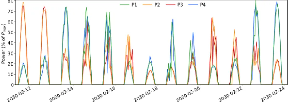
Fig. 4 depicts the resulting spatial variation of the solar GHI patterns (derived by GREECE) on the produced power from the optimal solar PV plants (location and size) whose placement is visible in Fig. 6 (b). P1 and P4 sites (P2 and P3) have similar patterns for they are located in the same solar potential cluster zone. Essentially, it shows how our GIS-RO approach manages real site spatial arrangement so that the global output power is robust through time from the optimal PV plants: impact of their RE intermittency on future network power management is limited.
Fig. 4: Normalized output power from solar PV sites of Fig. 6.
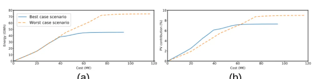
Fig. 5 gives information about (a) the volume of solar PV plants one may install within the region without threatening the power grid in the long-term, and (b) its corresponding final share in the energy mix. As long as both Pareto lines remain together in Fig. 5 (a), the solution is robust, i.e. power generation over time from selected plants fills up the same free energy volume regardless of the scenario: corresponding PV sites can be explored safely in the limits of their maximum capacity estimated by the RO. In contrast, once the best case reaches its plateau , and so Pareto lines split in half (around 40 Me), power generation no longer fills up the same volume. At this point, the more the energy generated in the worst case scenario, the more it exceeds the energy generation limit in the best case: the risk grows as much as the gap between both lines.
Finally, Fig. 6 evaluates the robustness of the investment according to spatio-temporal uncertainty on the resource: i) estimated GHI, energy potential (in blue), ii) its mitigation by a random uniform noise per hour and per parcel, between 0 and 10 % (in green) and iii) between 0 and 20 % (in red) respectively.
(a)
(b)
Fig. 5: Pareto charts for both scenarios with respect to (a) generated energy and (b) PV penetration.
The safety zone lies below a cost of 70 Me (C70), meaning that the selected PV sites are the same for all resource time series projections. Those sites are sorted by ascending parcel size area from the smallest (P1) to the largest (P4). The investment costs grow naturally when the optimal PV plant size grows within its corresponding parcel area (fractional knapsack optimization).
C70
P1 P2 P3 P4 P4
P1 P2
P4
Safety zone
(a) Pareto solution
(b) Corresponding PV sites in Guiana
Fig. 6: Robustness of the worst-case scenario solution with decreasing resource
6
Conclusion
In this paper we have proposed a two-step specification and novel computational approach of the spatio-temporal placement and energy planning problem. We ad-dressed key challenges of sustainable science in terms of spatial decision making and usage of complex contextual data, constraints and time series of resources. The presented GIS-RO framework allows for real world and large scale applica-tions to be solved through an integrated approach at the interface of GIS science, graph and robust optimization models and methods. The case study showed in particular the importance of taking into account actual resource patterns and al-lowing for fractional parcel selection to optimize power plants location and size, and thus optimize the power penetration at minimal cost. Current work includes its generalization to include the cost-effectiveness of energy storage considered not profitable to this date in Guiana, and the generalization to biomass resources that raises a complex temporal renewability issue of the resource.
References
1. Aguiar, R., Collares-Pereira, M.: TAG: A time-dependent, autoregressive, Gaus-sian model for generating synthetic hourly radiation. Solar Energy 49(3), 167–174
(1992).https://doi.org/10.1016/0038-092X(92)90068-L
2. Aguiar, R.J., Collares-Pereira, M., Conde, J.P.: Simple procedure for generating se-quences of daily radiation values using a library of Markov transition matrices.
So-lar Energy 40(3), 269–279 (1988).https://doi.org/10.1016/0038-092X(88)90049-7
3. Al Garni, H.Z., Awasthi, A.: Solar PV power plant site selection using a GIS-AHP based approach with application in Saudi Arabia. Applied Energy 206, 1225–1240
(2017).https://doi.org/10.1016/j.apenergy.2017.10.024
4. Al Garni, H.Z., Awasthi, A.: Solar PV power plants site
selec-tion: A review. In: Yahyaoui, I. (ed.) Advances in Renewable
Ener-gies and Power Technologies, chap. 2, pp. 57 – 75. Elsevier (2018).
https://doi.org/https://doi.org/10.1016/B978-0-12-812959-3.00002-2
5. Albarelo, T., Marie-Joseph, I., Primerose, A., Seyler, F., Wald, L., Linguet, L.: Optimizing the heliosat-II method for surface solar irradiation estimation with GOES images. Canadian Journal of Remote Sensing 41(2), 86–100 (2015). https://doi.org/10.1080/07038992.2015.1040876
6. Ali, S., Taweekun, J., Techato, K., Waewsak, J., Gyawali, S.:
GIS based site suitability assessment for wind and solar farms
in Songkhla, Thailand. Renewable Energy 132, 1360–1372 (2019).
https://doi.org/https://doi.org/10.1016/j.renene.2018.09.035
7. Barbosa, L., Bogdanov, D., Vainikka, P., Breyer, C.: Hydro, wind and solar power as a base for a 100% Renewable Energy supply for South and Central America.
PLoS ONE 12(3), 1–28 (2017).https://doi.org/10.1371/journal.pone.0173820
8. Ben-Tal, A., Nemirovski, A.: Robust solutions of uncertain linear programs. Oper. Res. L (25), 1–13 (1999)
9. Bogdanov, D., Breyer, C.: North-East Asian Super Grid for 100% renewable energy supply: Optimal mix of energy technologies for electricity, gas and heat supply options. Energy Conversion and Management 112, 176–190 (2016). https://doi.org/10.1016/j.enconman.2016.01.019
10. Bolwig, S., Bazbauers, G., Klitkou, A., Lund, P.D., Blumberga, A., Blumberga, D.: Review of modelling energy transitions pathways with application to energy system flexibility. Renewable and Sustainable Energy Reviews 101, 1–23 (2019). https://doi.org/10.1016/j.rser.2018.11.019
11. Breyer, C., Bogdanov, D., Aghahosseini, A., Gulagi, A., Child, M., Oyewo, A.S., Farfan, J., Sadovskaia, K., Vainikka, P.: Solar photovoltaics demand for the global energy transition in the power sector. Progress in Photovoltaics: Research and
Applications pp. 505–523 (2017).https://doi.org/10.1002/pip.2950
12. Breyer, C., Bogdanov, D., Komoto, K., Ehara, T., Song, J., Enebish, N.: North-East Asian Super Grid: Renewable energy mix and economics. Japanese Journal of
Ap-plied Physics 54(8S1), 08KJ01 (2015).https://doi.org/10.7567/JJAP.54.08KJ01
13. Castro-Santos, L., Garcia, G.P., Sim˜oes, T., Estanqueiro, A.: Planning
of the installation of offshore renewable energies: A GIS approach of
the Portuguese roadmap. Renewable Energy 132, 1251–1262 (2019).
https://doi.org/10.1016/j.renene.2018.09.031
14. Chinneck, J.W., Ramadan, K.: Linear programming with interval coefficients. J. Operational Research Society (51 (2)), 209 – 220 (2000)
15. CTG: Programmation pluriannuelle de l’´energie (PPE) 2016-2018 et 2019-2023 de
16. Dotzauer, M., Pfeiffer, D., Lauer, M., Pohl, M., Mauky, E., B¨ar, K., Sonnleitner,
M., Z¨orner, W., Hudde, J., Schwarz, B., Faßauer, B., Dahmen, M., Rieke, C.,
Herbert, J., Thr¨an, D.: How to measure flexibility – Performance indicators for
demand driven power generation from biogas plants. Renewable Energy 134, 135–
146 (2019).https://doi.org/10.1016/j.renene.2018.10.021
17. EDF: Syst`emes ´energ´etiques insulaires Guyane - bilan pr´evisionnel de l’´equilibre
of-fre / demande d’´electricit´e. Tech. rep., EDF - Direction des Syst`emes ´Energ´etiques
Insulaires, Paris, France (2017)
18. EDF: Open Data EDF Guyane (2019), https://opendata-guyane.edf.fr/pages/
home/, accessed: 2019-04-30
19. Ferrer-Mart´ı, L., Domenech, B., Garc´ıa-Villoria, A., Pastor, R.: A MILP model to design hybrid wind-photovoltaic isolated rural electrification projects in develop-ing countries. European Journal of Operational Research 226(2), 293–300 (2013). https://doi.org/10.1016/j.ejor.2012.11.018
20. Fillol, E., Albarelo, T., Primerose, A., Wald, L., Linguet, L.: Spatiotemporal indica-tors of solar energy potential in the Guiana Shield using GOES images. Renewable
Energy 111, 11–25 (2017).https://doi.org/10.1016/j.renene.2017.03.081
21. GDAL/OGR contributors: GDAL/OGR Geospatial Data Abstraction software
Li-brary. Open Source Geospatial Foundation (2019),https://gdal.org
22. Gervet, C., Atef, M.: Optimal allocation of renewable energy parks: a two-stage optimization model. RAIRO-Operations Research (47), 125–150 (2013). https://doi.org/10.1051/ro/2013031
23. Hache, E., Palle, A.: Renewable energy source integration into power
networks, research trends and policy implications: A bibliometric and
research actors survey analysis. Energy Policy 124, 23–35 (2019).
https://doi.org/10.1016/j.enpol.2018.09.036, https://doi.org/10.1016/j.enpol.
2018.09.036
24. Heydari, A., Askarzadeh, A.: Optimization of a biomass-based
pho-tovoltaic power plant for an off-grid application subject to loss of
power supply probability concept. Applied Energy 165, 601–611 (2016). https://doi.org/10.1016/j.apenergy.2015.12.095
25. Holmgren, W.F., Hansen, C.W., Mikofski, M.A.: Pvlib Python: a Python package for modeling solar energy systems. Journal of Open Source Software 3(29), 884
(month 2018).https://doi.org/10.21105/joss.00884
26. IGN: BD TOPO R
Version 2.2 - Descriptif de contenu. Institut G´eographique
Na-tional, Paris, France (2018), http://professionnels.ign.fr/doc/DC BDTOPO 2-2.
27. Jarvis, A., Reuter, H., Nelson, A., Guevara, E.: Hole-filled SRTM for the globe
Version 4, available from the CGIAR-CSI SRTM 90m Database http://srtm.csi.
cgiar.org. Tech. rep. (2008)
28. Juffe-Bignoli, D., Bingham, H., MacSharry, B., Deguignet, M., Milam, A., Kingston, N.: World database on protected areas – User manual 1.4. United Nations Environment Programme - World Conservation Monitoring Centre, 219 Hunting-don Road, Cambridge, UK (2016)
29. Karypis, G.: METIS: A software package for partitioning unstructured graphs, par-titioning meshes, and computing fill-reducing orderings of sparse matrices. Depart-ment of Computer Science & Engineering, University of Minnesota, Minneapolis, MN 55455 (2013)
30. Karypis, G., Kumar, V.: A fast and highly quality multilevel scheme for parti-tioning irregular graphs. SIAM Journal on Scientific Computing 20(1), 359–392 (1999)
31. NREL: Distributed generation renewable energy estimate of costs.https://www.
nrel.gov/analysis/tech-lcoe-re-cost-est.html(2016)
32. ONF Guyane: Programme r´egional de mise en valeur foresti`ere pour la production
de bois d’œuvre - p´eriode 2015-2019. Tech. rep., Direction R´egionale ONF Guyane
(2015)
33. ONF Guyane: Occupation du sol en 2015 sur la bande littorale de la Guyane et
son ´evolution entre 2005 et 2015. Direction R´egionale ONF Guyane (2017)
34. Ozdemir, S., Sahin, G.: Multi-criteria decision-making in the location
se-lection for a solar PV power plant using AHP. Measurement:
Jour-nal of the InternatioJour-nal Measurement Confederation 129, 218–226 (2018). https://doi.org/10.1016/j.measurement.2018.07.020
35. Pfenninger, S., Hawkes, A., Keirstead, J.: Energy systems modeling for twenty-first century energy challenges. Renewable and Sustainable Energy Reviews 33, 74–86
(2014).https://doi.org/10.1016/j.rser.2014.02.003
36. Purkus, A., Gawel, E., Szarka, N., Lauer, M., Lenz, V., Ortwein, A., Tafarte, P.,
Eichhorn, M., Thr¨an, D.: Contributions of flexible power generation from biomass
to a secure and cost-effective electricity supply – a review of potentials, incen-tives and obstacles in Germany. Energy, Sustainability and Society 8(1) (2018). https://doi.org/10.1186/s13705-018-0157-0
37. Ramirez Camargo, L., Stoeglehner, G.: Spatiotemporal modelling for integrated spatial and energy planning. Energy, Sustainability and Society 8(1), 32 (2018). https://doi.org/10.1186/s13705-018-0174-z
38. Remund, J., M¨uller, S., Kunz, S., Huguenin-Landl, B., Studer, C., Cattin, R.:
Meteonorm Handbook part II: Theory, Global Meteorological Database Version
7 Software and Data for Engineers, Planers and Education (2018), http://www.
meteonorm.com
39. Sabo, M.L., Mariun, N., Hizam, H., Mohd Radzi, M.A., Zakaria, A.: Spa-tial matching of large-scale grid-connected photovoltaic power generation with utility demand in Peninsular Malaysia. Applied Energy 191, 663–688 (2017). https://doi.org/10.1016/j.apenergy.2017.01.087
40. Siyal, S.H., M¨ortberg, U., Mentis, D., Welsch, M., Babelon, I., Howells,
M.: Wind energy assessment considering geographic and environmental re-strictions in Sweden: A GIS-based approach. Energy 83, 447–461 (2015). https://doi.org/10.1016/j.energy.2015.02.044
41. Sultana, A., Kumar, A.: Optimal siting and size of bioenergy facilities using geographic information system. Applied Energy 94, 192–201 (2012). https://doi.org/10.1016/j.apenergy.2012.01.052
42. Teixeira, T.R., Ribeiro, C.A.A.S., dos Santos, A.R., Marcatti, G.E., Lorenzon, A.S., de Castro, N.L.M., Domingues, G.F., Leite, H.G., da Costa de Menezes, S.J.M., Mota, P.H.S., de Almeida Telles, L.A., da Silva Vieira, R.: Forest biomass power plant installation scenarios. Biomass and Bioenergy 108, 35 – 47 (2018). https://doi.org/https://doi.org/10.1016/j.biombioe.2017.10.006
43. van der Walt, S., Colbert, S.C., Varoquaux, G.: The numpy array: A structure for efficient numerical computation. Computing in Science Engineering 13(2), 22–30
(March 2011).https://doi.org/10.1109/MCSE.2011.37
44. Wang, Q., M’Ikiugu, M., Kinoshita, I., Wang, Q., M’Ikiugu, M.M., Kinoshita, I.: A GIS-Based Approach in Support of Spatial Planning for Renewable Energy: A Case Study of Fukushima, Japan. Sustainability 6(4), 2087–2117 (apr 2014). https://doi.org/10.3390/su6042087
45. Watson, J.J., Hudson, M.D.: Regional Scale wind farm and solar farm suitabil-ity assessment using GIS-assisted multi-criteria evaluation. Landscape and Urban
Planning 138, 20–31 (2015).https://doi.org/10.1016/j.landurbplan.2015.02.001
46. Woo, H., Acuna, M., Moroni, M., Taskhiri, M.S., Turner, P.: Optimizing the location of biomass energy facilities by integrating Multi-Criteria Analysis (MCA) and Geographical Information Systems (GIS). Forests 9(10), 1–15 (2018). https://doi.org/10.3390/f9100585