HAL Id: hal-01217215
https://hal.archives-ouvertes.fr/hal-01217215
Submitted on 20 Oct 2015
HAL is a multi-disciplinary open access
archive for the deposit and dissemination of
sci-entific research documents, whether they are
pub-lished or not. The documents may come from
teaching and research institutions in France or
abroad, or from public or private research centers.
L’archive ouverte pluridisciplinaire HAL, est
destinée au dépôt et à la diffusion de documents
scientifiques de niveau recherche, publiés ou non,
émanant des établissements d’enseignement et de
recherche français ou étrangers, des laboratoires
publics ou privés.
T-P Interval Estimation in case of Overlapping Waves
Hervé Rix, Aline Cabasson, Michal Kania, Olivier Meste
To cite this version:
Hervé Rix, Aline Cabasson, Michal Kania, Olivier Meste. T-P Interval Estimation in case of
Overlap-ping Waves. Computing in Cardiology, Sep 2015, Nice, France. �hal-01217215�
T-P Interval Estimation in case of Overlapping Waves
Hervé Rix
1, Aline Cabasson
1, Michal Kania
2,3, Olivier Meste
11
Lab. I3S, Univ. Nice Sophia Antipolis, CNRS, Sophia Antipolis, France
2Nalecz Institute Biocybern. & Biomed. Eng., PAS, Warsaw, Poland
3
Electrophysiology and Heart Modeling Institute (IHU LIRYC), Bordeaux, France
Abstract
Assuming two positive overlapping signals, with known shapes, the proposed method estimates the distances between their mean positions, width and area ratios. The data are two profiles representing the component shapes: no parametric model is assumed. The algorithm seeks shape equality between a linear combination of observation and first component, and the second component, in function of the area ratio. At the minimum shape difference the three parameters (distance between components, scaling factor and area ratio) are estimated. After theory, simulations are presented on Gaussian signals. Then, the method was applied on ECG signals from BSPM device during exercise on healthy people. The aim is mainly to get time distance between each T-wave and the P-wave of the following beat, on a given lead, in case of overlapping. Shape and width of the T-wave were shown to be constant before P-wave interference, which allowed taking such a real T-wave as first component model. Assumption of the same shape for the second component gave good results, as can be viewed on the reconstructed signals.
1. Introduction
In this paper we are interested in the observation of signals which are produced by the overlapping of two positive components. In two situations the estimation becomes very difficult or impossible: either when the components are much fused, i.e. with a bad separation, even with a high Signal to Noise Ratio (SNR), e.g. chromatography, spectroscopy [1], or when we have a poor SNR. The influence of noise is generally preponderant in biomedical signals like exercise ECG recordings. This case is illustrated in this paper, where a method is presented which is able to separate the T and P waves, in case of overlapping, with good reconstruction capability. In [2], a method to subtract the overlapping T-wave influence was
proposed for a better estimation of PR interval durations, but the waves were not reconstructed. An alternative is proposed in our method which will check distances between signal shapes, without assuming any parametric model. In the following section, the method is presented.
2.
Material and methods
After giving our hypotheses on shape analysis, the model of the observed signals and the assumed data, the theory of the proposed method is stated, followed by the description of the estimation algorithm.
2.1.
Hypotheses and model
Signal shape equality
Signals s(t) and v(t), functions of the real variable t, will be the same shape if and only if we can write:
(1) From (1) we can deduce the following equivalent relation:
(2) Often, in applications, when a base line is subtracted, the parameter c is assumed to be zero.
Shape difference
Measuring a difference between two shapes needs a distance, or at least a similarity criterion. A method based on shape analysis, the Distribution Function Method (DFM) has been proposed in [3]. Its ability to detect very small shape differences, between positive signals, has been applied to detect impurities by chromatography [4] and to analyze and model nonlinearity in chromatograph response [5]. It has also been applied in the biomedical domain [6-8].
The data and the model
The data consist of a real signal s(t), proportional to the first component, another one v(t) which is the same shape as the second component, and the observed signal y(t), all in discrete form. We also
0 , 0 ) ( ) (t ksat b c k a v k c c k k c a b t v k t s() ' ( ) ' ' 1, '
assume the areas under s(t) and v(t) are equal. It is important to emphasize that no parametric model is assumed for s(t) and v(t). We need only their shapes represented by experimental records. So, the model can be defined by the following equation:
(3) In this equation, C is a constant and n(t) a noise assumed to be zero mean and independent of the signals. The problem is to estimate parameters k, a and d which are respectively the area ratio, the scaling factor and the separation between components. In fact this last parameter is equal to the distance between the mean positions (gravity centres) of s(t) and v(t), when a=1 or when the mean position of s(t) is taken as the origin of variable t. Let us call δ this distance, the relation between δ, d, a, and the mean position of s(t), say tm(s), is :
(4) In this paper, tm(s) is always the origin of variable t, so d will be equal to δ. In the following, the proposed method for the separation of two overlapping signals is stated.
2.2.
Theory
Neglecting the noise, equation (3) becomes: (5) Capital letters will be used for the integral functions. The adjunction of a star to a function means this function is normalized by the integral of the signal. For example:
Writing (5) on normalized integral functions gives: (6)
Putting , it is a convex combination of
the form:
(7) The involved signals being positive on their supports, these normalized integral functions are distribution functions (DF).
Equation (6) can be written in the form: (8)
where: .
Putting,
(9)
let us consider this right hand side of (8) as a function with parameter β: this linear combination of two DFs, which is not convex (β >1), can be shown to be a DF if 1< β <βsup, βsup depending on the involved signals.
There exits one value β* so that this function and V*
are linked by an affine function whose parameters give estimates of a and d. Checking this link is equivalent to check the both functions whose
normalized integrals are V* and H
β are the same shape. Then the problem becomes the minimization of a shape difference, measured using DFM, which is recalled in the next section.
2.3.
Estimation algorithm
The power of the method is first shown by simulation, assuming the two components are the same shape. The aim of the paper is not to give a detailed study of the estimation accuracy when the three parameters (a, d, k) are made to vary in large sets of values, and for a lot of SNRs. The simulation study is coherent with the application.
Computing the shape difference
Assuming Hβ is a DF and recalling DFM, for any
value z, 0< z <1, we can write:
(12) This function is an increasing function, depending on β which can be written as the composition of the
inverse function of S* and H
β :
(13) This function is an affine function in case of shape equality, i.e. β = β*, whose equation is:
(14) In any case, fitting the least mean square line on gives a root mean square error (r.m.s.e.) which will represent our shape difference. Practically, interval (0, 1) is sampled with the values i/100, i being an integer going from 0 to 100, leading to the corresponding abscissas ti and ti’. In fact the fitting will be done for the index values i going from 5 to 95, to avoid problems of inversion when the slopes of de normalized integral functions are too small.
Synchronization of the first component
Coming back to the model and hypotheses (sections 2.1, 2.2) we assume to have a profile s(t) which is proportional to the first component, i.e. with the same mean position and the same width. In fact, the hypothesis that the position of the first component is exactly known is realistic in some applications like chromatography or spectroscopy. It is not true in our application. Only the hypothesis of constant width, checked before overlapping, was assumed. For this reason, a new parameter was added in the shape ) ( )) ( ) ( ( ) ( nt a d t v a k t s C t y d s t a 1)m( ) ( )) ( ) ( ( ) ( a d t v a k t s C t y t d y t Y() ( ) d y d y t Y t ) ( / ) ( ) ( * ) ( 1 ) ( 1 1 ) ( * * * a d t V k k t S k t Y ) 1 /( k k ) ( ) ( ) 1 ( ) ( * * * a d t V t S t Y ) ( ) 1 ( ) ( ) ( * * * t S t Y a d t V 1 / 1 ) ( ) 1 ( ) ( ) ( * * t S t Y t H ) ( ' ) ' ( ) ( * t t t S t H z H S*)1 ( a d t t' ( )/ ) ( ' t t
minimization that is a possible error, ε, in the position of s(t). So s(t) becomes s(t- ε), and S*(t) becomes S*(t- ε) in the computation of equation (9).
The main steps of the estimation
Assuming equal shape components, a Gaussian profile is used for this shape, in the simulation study. Then, equation (8) becomes for a given delay error ε: (8’) Now, let us consider the right hand side of (8’) as a parameterized function given in equation (9’).
(9’) For each ε value, we are looking for the value of β which minimizes the shape difference, designed by variable DELTA1, between this function (more precisely its derivative) and the reference signal s(t-ε). So, the simulation program is built on three loops. The first, indexed by I (going from 1 to 30) allows producing sequences of a random Gaussian noise with a given SNR, added to the observation signal y(t). Inside this first loop the second one, indexed by K (going from 1 to 101), introduces the delay ϵ on the first component model, varying in the range of one standard deviation. Lastly, for each value of I and K,
the shape distance DELTA1(β,ε) between Hβ,ε and S*
is computed when parameter β is increased from 1 to
a value where Hβ,ε remains a DF, by steps of 0.01. As
explained before, this shape difference needs to
compute the inverse function (S*)-1 designed by t’ and
the inverse function (Hβ,ε)-1 designed by t, and to make a linear fitting: t = a1 t’ + a2.
When the r.m.s.e. reaches a minimum value attributed to β*, the parameters a
1 and a2 of the least mean square line are respectively the estimations of parameters “a” and “d”, for the delay ε defined by index K, and for the noise sequence numbered by index I. The minimization of DELTA1 in function of K, obtained for K=K*, gives an estimation of the scaling factor and the distance between the components. Renewing these estimations for several noisy trials, allows obtaining statistics on the estimations. Coming to the last parameter k, its relation with β*, i.e. the β value where a and d are estimated, leads to a natural estimation, given by:
(15) For high levels of noise or small values of parameter d, the curve of DELTA1, in function of K (i.e. ε) is flat: the value of the minimum is quite constant in a large range around K*, but the error on the position K* is high. To reduce this error, another minimization was done. For each K value, we can obtain the
reconstructed signal yrec(K) and compute the
difference in shape DELTA2(K) between yrec(K) and
the observation y. The second minimization, in function of parameter K, sensitive to the
synchronization of the first component with its model, gives significantly better results, as can be checked in our simulation study. Minimizing DELTA1 in function of the both parameters β and ε is referred as “Method 1”; using DELTA1 in function of β, for a given ε, and then DELTA2 for the final estimation is referred as “Method 2”.
3.
Simulation results
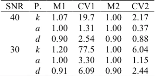
The following examples have been chosen to illustrate the power of the proposed method first when the separation is very poor (d=0.9) with high SNR (Table 1), and then when SNR is low (10 and 5 dB) with values of the parameters in ranges corresponding to our application on ECG (Table 2, Table 3). Table 1. Parameter estimation when k=1, a=1, d=0.9, SNR=40 and 30 dB: Means M1, M2, and Coefficients of Variation (in %) CV1, CV2 using “Method 1” and “Method 2” (see in the text).
SNR P. M1 CV1 M2 CV2 40 k 1.07 19.7 1.00 2.17 a 1.00 1.31 1.00 0.37 d 0.90 2.54 0.90 0.88 30 k 1.20 77.5 1.00 6.04 a 1.00 3.30 1.00 1.15 d 0.91 6.09 0.90 2.44 Table 2. See legend Table 1 with k=0.6, a=0.8, d=2.2, SNR=10 and 5 dB. SNR P. M1 CV1 M2 CV2 10 k 0.62 15.4 0.60 5.69 a 0.81 7.82 0.80 4.92 d 2.21 1.90 2.21 1.04 5 k 0.67 28.4 0.60 12.2 a 0.80 13.7 0.78 8.93 d 2.23 3.26 2.21 2.68 Table 3. See legend Table 1 with k=0.6, a=1.2, d=2.7, SNR=10 and 5 dB. SNR P. M1 CV1 M2 CV2 10 k 0.61 10.9 0.60 7.35 a 1.20 7.57 1.19 5.37 d 2.68 2.18 2.69 2.17 5 k 0.64 17.3 0.60 8.60 a 1.22 9.64 1.19 6.85 d 2.67 4.00 2.70 3.19 In Table 3, parameters d and a were changed from Table 2, with the same resolution proportional to d/(1+a). Method 2 is clearly the better.
) ( ) 1 ( ) ( ) ( * * * t S t Y a d t S ) ( ) 1 ( ) ( ) ( * * , t Y t S t H ) 1 /( 1 * * k
4. Application to exercise ECG
The following results come from records of High Resolution ECG obtained on lead V5 during an exercise test on healthy people. In a first step, the differences in shape and width of the T wave, from beat to beat, were found constant in mean, until T and P waves remain separated. Thus, the last T wave (number 680) was taken to model the first component. The width and the shape of the second component, i.e. the P wave, vary along the test. Due to high noise level the shape was assumed to be the same as T wave shape.
Figure 1. T-P interval in function of beat number (dotted line) and RR curve minus 200 ms.
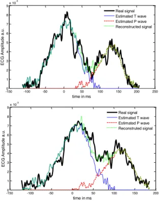
Figure 2. Examples of signal reconstruction when the component separation is around 2.9 (up) and 2.0 (bottom); unity=half width at half height of T wave.
In Figure 1, the variation of T-P interval is presented: the curve built from 30 estimations (dotted line) can be compared to the RR curve (minus 200 ms) at the same beats. For this preliminary study, the signal segmentation was made by hand. In Figure 2, two examples of such estimations are shown on the reconstructed signal and the estimated components.
5. Conclusions
On one hand, the simulation study showed that the presented method has potential application domains going from spectroscopy to biomedical signal analysis. On another hand, the preliminary results obtained on an exercise ECG show potential applications to stress test analysis. The separation of P wave from T wave could bring valuable information hidden by the overlapping, and could also improve the estimation of PR interval duration.
References
[1] Baruya A, Maddams WF. An examination of the uniqueness of Gaussian and Lorentzian profiles. Appl. Spectrosc., 1978; 32(6): 563-566.
[2] Cabasson A, Meste O, Blain G, Bermon S. Quantifying the PR interval pattern during dynamic exercise and recovery. IEEE Trans Biomed Eng. 2009; 56(11): 2675-83.
[3] Rix H, Malengé JP. Detecting small variations in Shape. IEEE Trans Systems, Man and Cybernetics 1980;10: 90-96.
[4] Rix H, Malengé JP. Detection of an impurity (1%) at low resolution (0.25). Journal of High Resolution Chromatography and Chromatography Communications 1980; 3(4): 172-176.
[5] Excoffier JL, Jaulmes A, Vidal-Madjar C, Guiochon G. Characterization of small variations in profiles of chromatographic elution peaks and effect of nonlinearity of sorption isotherm. Anal Chem. 1982; 54 (12): 1941–1947.
[6] Khaddoumi B, Rix H, Meste O, Fereniec M, Maniewski R. Body Surface ECG Signal Shape Dispersion. IEEE Trans Biomed Eng. 2006; 53(12):2491-2500.
[7] Fereniec M, Maniewski R, Karpinski G, Opolski G, Rix H. High-resolution multichannel measurement and analysis of cardiac repolarization. Biocybernetics and Biomedical Engineering 2008; 28(3): 61-69.
[8] Kania M, Rix H, Fereniec M, Zavala-Fernandez H, Janusek D, Mroczka T, Stix G, Maniewski R. The effect of precordial leads displacement on ECG morphology. Med Biol Eng Comput. 2014; 52(2): 109– 119.
Address for correspondence:
Hervé Rix. Laboratoire I3S – UMR7271 - CS 40121 - 06903 Sophia Antipolis, cedex, France.
600 800 1000 1200 1400 1600 1800 2000 100 150 200 250 300 350 Beat number ms -1500 -100 -50 0 50 100 150 200 250 1 2 3 4 5 6 7 8 9x 10 -3 time in ms EC G Am p lit u d e a .u . Real signal Estimated T wave Estimated P wave Reconstructed signal -1500 -100 -50 0 50 100 150 200 1 2 3 4 5 6 7 8 9x 10 -3 time in ms EC G Am p lit u d e a .u . Real signal Estimated T wave Estimated P wave Reconstruted signal