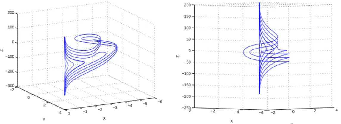
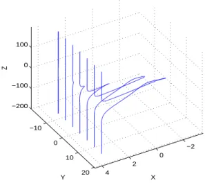
Scattering of cosmic strings by black holes: loop formation

The analysis suggests a black hole mass threshold for powerful radio emission and also properly distinguishes core-dominated and lobe-dominated quasars, in accordance with the

Dans le cadre de la mondialisation galopante, L’environnement fait l’objet de préoccupations engagées, tant au niveau national qu’international, en raison de

In this paper we describe the experiment which has verified the black body character of the spectrum of the cosmic background radiation on the high frequency side of the peak

cases are considered : the diffraction of an incident plane wave in section 3 and the case of a massive static scalar or vector field due to a point source. at rest

When studying the problem of linear stability, such growing modes therefore cannot appear as the asymptotic behavior of a gravitational wave; in fact, one can argue, as we shall do

Starting from an FIR-selected sample, the incompleteness in accretion luminosity might be eval- uated by looking at the distribution of flux ratio between accretion flux S accr

Bien que les résultats de calcul théorique en utilisant la fonctionnelle MPW1PW91 avec des jeux de base bien adaptés 6-311G et Lanl2DZ aient trouvé des valeurs acceptables dans

Conclusion Dans ce chapitre, on a présenté quelques notions sur les cellules solaires à base des semiconducteurs III-nitrures et III-V de type monojonction et multijonction, qui