HAL Id: hal-00359464
https://hal.archives-ouvertes.fr/hal-00359464
Preprint submitted on 7 Feb 2009
HAL is a multi-disciplinary open access
archive for the deposit and dissemination of
sci-entific research documents, whether they are
pub-lished or not. The documents may come from
teaching and research institutions in France or
abroad, or from public or private research centers.
L’archive ouverte pluridisciplinaire HAL, est
destinée au dépôt et à la diffusion de documents
scientifiques de niveau recherche, publiés ou non,
émanant des établissements d’enseignement et de
recherche français ou étrangers, des laboratoires
publics ou privés.
Structure of neighborhoods in a large social network
Alina Stoica, Christophe Prieur
To cite this version:
Alina Stoica, Christophe Prieur. Structure of neighborhoods in a large social network. 2009.
�hal-00359464�
Structure of neighborhoods in a large social network
Alina Stoica
Orange Labs and LiafaParis, France
stoica@liafa.jussieu.fr
Christophe Prieur
Liafa Paris, Franceprieur@liafa.jussieu.fr
ABSTRACT
We present here a method for analyzing the neighborhoods of all the vertices in a large graph. We first give an algorithm for characterizing a simple undirected graph that relies on enumeration of small induced subgraphs. We make a step further in this direction by identifying not only subgraphs but also the positions occupied by the different vertices of the graph. We are thus able to compute the roles played by the vertices of the graph, roles found according to a new definition that we introduce. We apply this method to the neighborhood of each vertex in a 2.7M vertices, 6M edges mobile phone graph. We analyze how the contacts of each person are connected to each other and the positions they occupy in the neighborhood network. Then we compare their quantity of communication (duration and frequency) to their positions, finding that the two are not independent. We finally interpret and explain the results using social studies on phone communications.1
Categories and Subject Descriptors
H.2.8 [Database Management]: Database Applications—
Data Mining; G.2.2 [Discrete Mathematics]: Graph
The-ory—Graph algorithms; J.4. [Computer Applications]: Social and Behavioral Sciences—Sociology
General Terms
Algorithms, Human Factors, Measurement, Theory
Keywords
social networks, roles, patterns, complex networks, personal networks
1.
INTRODUCTION
The study of social networks has changed a lot since the early pioneering works of anthropologists who decided to focus 1Supplementary material is available online at www.liafa.jussieu.fr/˜stoica/neighborhoods
on relationships instead of individuals [7, 4, 3]. After the technical framework of social network analysis was settled in the 1970’s by the combination of mathematical tools such as graph theory, algebra and statistics [26, 8, 32, 33], the field has been again shaken with the exponential growing of the size of relational databases coming with the development of communication tools. The tremendous research activity on the structure of the World-Wide Web [14, 11, 12] that have pre-dated Google’s PageRank algorithm [9] have given birth to a new object of study, namely complex networks, due to the common properties found to be shared not only by the graph of the WWW [2, 34] but also by many networks appearing in various contexts (biology, linguistics, economics and, of course, social networks) [29, 6].
There is thus a wide gap between these kinds of studies of the global structure of huge networks and qualitative studies of personal networks, sometimes built from face-to-face in-terviews (for a historical survey of this trend, see [35]), even though more and more such studies now take as data per-sonal networks scraped from internet’s social network ser-vices [18]. Inbetween, the classical problem of identifying roles in a (possibly quite large) network, introduced in the 1970’s as one of the main tools of social network analysis [37], relies on the fact that some nodes have similar po-sitions in the sense that they are linked to the same other nodes, which is defined as the so-called structural equivalence of nodes, or the more general notion of regular equivalence, where two nodes are equivalent if the neighbors of the two are equivalent to each other [5].
Our work is at the intersection of these three research trends: we study the roles of nodes in the personal networks of all individuals of a large (thus ‘complex’) network. In [31] (in French), we already compared to a classical ethnographic study what can be achieved in terms of qualitative analy-sis with such a large-scale (2 million) collection of personal networks.
Now to address the issue of roles, we devised a method rely-ing on a very popular data minrely-ing problem: the search for frequent subgraphs in a given (possibly large) graph. On this issue, some authors considered that frequent subgraphs are the ones that appear in a given graph (or set of graphs) more often than a chosen threshold. Some algorithms [19, 21] extend the apriori-based candidate generation-and-test approach [1], while others [5, 39] use a pattern-growth ap-proach [15]. More recently, several algorithms have been
proposed for significant graph pattern mining [17, 38]. Milo
et al [28] used another approach to find interesting patterns.
They compared the frequency of subgraphs with the ones appearing in randomly generated graphs that share some properties of the network. Several methods for an efficient counting of subgraphs with a given maximal size have been proposed since [36, 20]. Here, we apply the method intro-duced by Wernicke to the neighborhood of each vertex of the given network. This allows us to compute in the same time the subgraphs that appear more frequently than a chosen threshold and the ones that appear more frequently than in randomly generated networks. Unlike previously done, to our knowledge, we are also able to identify the positions that the different neighbors occupy and therefore the roles they play.
We apply this method to a large network built from mobile phone communications. Of course, there are many forms of social interactions between two people: face-to-face in-teractions, emails, instant messages, (fixed) telephone, the mobile phone communications capturing only a subset of the underlying social network. However, studies on the strength of ties have shown that mobile phone is among the most inti-mate communication tools and moreover that people a mo-bile phone conversation suggests a certain relation between the two individuals, given that there aren’t any listings of mobile phone numbers. Moreover, people that contact each other via one communication tool tend to communicate via other ones as well [16], hence the relevance of analyzing a mobile phone network in the search of understanding the underlying social network.
Different properties have been already identified in large mo-bile phone networks [30, 10]. Onnela et al [30] show with no surprise that the distributions of degree and of the duration of calls are power-laws. More strikingly they also give a def-inition for the strength of ties depending on the duration of calls and they analyze the connection between the strength and the connectivity or the community structure.
As in complex network studies, all of these properties are global, characterizing the structure of the mobile phone graph as a whole. Here, our aim is to identify the local structure, the way the persons contacted by a given individual (ego) are connected to each other relatively to their ”importance” to ego. In order to do that, we use the frequency and the total duration of communications between ego and each of his contacts.
The paper is organized as follows. After recalling some ba-sic definition on graphs (Section 2), we detail in Section 3 a formal framework to address the issue of characterizing a graph in terms of a position equivalence along with an algo-rithm to do it. The main algoalgo-rithm to characterize all the neighborhoods of a large graph is given in Section 4 and in Section 5 we apply it to a mobile phone graph and discuss the results by comparing them to an ethnographic study on communication tools.
2.
PRELIMINARIES
Let G = (V, E) be a graph; V is the set of its vertices, E ⊆ V × V is the set of its edges. We define its size as |V |, the number of its vertices. Two vertices u, v ∈ V are
adjacent in G if (u, v) ∈ E. The graph G is undirected if,
for all u, v ∈ V , there is no difference between (u, v) and (v, u), it is connected if there exists a finite path between every two vertices and it is simple if there is no multiple edge and no self-loop ((v, v) /∈ E, for all v ∈ V ). For a vertex v ∈ V , we denote by N (v) = {u ∈ V, (u, v) ∈ E} its
neighborhood, by N [v] = N (v) ∪{v} its closed neighborhood
and by d(v) = |N (v)| its degree. The betweenness centrality [13] of a vertex v is defined as c(v) =Ps,t∈VG δv(s, t)
δ(s, t) where δ(s, t) denotes the number of shortest paths from s to t and δv(s, t) denotes the number of shortest paths from s to t that pass through v.
Two graphs G = (VG, EG) and H = (VH, EH) are
isomor-phic if and only if there exists a bijective function ϕ : VG→ VH (called isomorphism of G and H) such that any two vertices u and v are adjacent in G if and only if ϕ(u) and ϕ(v) are adjacent in H. When G and H are one and the same graph, the function ϕ is called automorphism of G. The graph isomorphism is an equivalence relation on graphs so it partitions the class of graphs into equivalence classes, called isomorphism classes.
Given a graph G = (VG, EG), a graph H = (VH, EH) is a subgraph of G if VH ⊆ VG and for all u, v ∈ VH, if (u, v) ∈ EH then (u, v) ∈ EG. H is an induced subgraph of G (denoted by H ֒→ G) if VH ⊆ VGand for all u, v ∈ VH, (u, v) ∈ EH if and only if (u, v) ∈ EG.
For a graph G and an positive integer k, Wernicke [36] pro-posed an algorithm that efficiently enumerates all the con-nected induced subgraphs of G with exactly k vertices. This algorithm, called ESU (G, k), starts with a vertex of G and adds neighboring vertices until a set of k vertices is obtained, hence a connected induced subgraph with k vertices. The neighboring vertices must satisfy certain conditions in order to be added to the already selected ones. This guarantees that each subgraph is listed exactly once.
3.
A CHARACTERIZATION OF GRAPHS
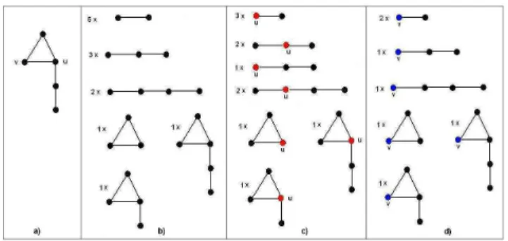
This section introduces a method to characterize a graph and its vertices. Given a graph, we enumerate all its connected induced subgraphs with size at most 5 and we group them into isomorphism classes. Then, for each vertex of the graph, we compute the position it occupies in each one of the found subgraphs. For example, for the graph in Figure 1 a, the number of its different induced subgraphs and the positions occupied by the vertices u and v are presented in Figure 1 b, c and d respectively.
3.1
Definitions
Given a graph G and a vertex v of G, we call neighb-degree of v, denoted by nd(v) = Pu∈N[v]d(u), the sum between its degree and the degrees of its neighbors. We call degrees
combination of the graph G the ascending sorted list of the
neighb-degrees of its vertices. Note that for a graph G with n vertices and m edges one compute the neighb-degrees of all the vertices of G in O(m) time, then its degrees combination in O(n · logn) time.
Given two graphs G and H and two vertices u ∈ VGand v ∈ VH, we say that u and v are position equivalent if there exists
Figure 1: A graph (a), its connected induced sub-graphs (b) and the positions of the vertices u (c) and v (d).
an isomorphism ϕ of G and H such that ϕ(u) = v. When G and H are one and the same graph, the position equivalence is the automorphic equivalence. In the isomorphism class C of a graph G, the set of all vertices is partitioned by the position equivalence into equivalence classes, called the
position classes in C; we denote by P (C) this set.
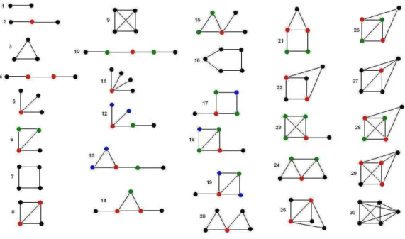
We denote by G the class of all undirected simple graphs, by C its isomorphism classes and by P = ∪C∈CP (C) the set of all the positions; Gk, Ck and Pk are the restrictions of these sets to connected graphs with at most k vertices and at least 1 edge. We call the 30 non-isomorphic graphs with size at most 5 (i.e. the graphs in C5) patterns. In Figure 2 is represented the set of patterns such that, for each pattern, each color corresponds to a different position class; there are 73 position classes in C5. We sort in ascending order the position classes of a same pattern by their betweenness centrality, then by their degree. We call peripheral the first position class in this order and central the last one. The position classes that are not central nor peripheral or are both central and peripheral are called intermediate. We define the function Sub : G × C → N such that, for a graph G and an isomorphism class C, Sub(G, C) counts the number of induced subgraphs of G that belong to C :
Sub(G, C) = |{H st H ֒→ G and H ∈ C}|.
We define the function P os : G × P × ∪G∈GVG → N such that for a graph G, a position class P and a vertex v ∈ VG, P os(G, P, v) counts the number of subgraphs of G that contain v in the position P :
P os(G, P, v) = |{H st H ֒→ G, v ∈ VH, P is a position class in the isomorphism class of H and v ∈ P }|. Subkand P oskare the restrictions of these functions to the sets Ckand Pkrespectively.
A new definition of social roles. We introduce here a new definition of equivalence of vertices in order to identify actors that play the same social role. We consider that ver-tices with the same role must have the same positions with regard to the vertices situated at a certain maximal distance from them. In other words, they must connect in the same way to the vertices around them.
Given a graph G with n vertices and a vertex v ∈ VG, we
call position vector of v in G the vector P s(v) such that P s(v)[P ] = P os(G, P, v), for each position class P ∈ P. The k−position vector of v, denoted by P sk(v), is the vec-tor computed only for the position classes in Pk. Given two vertices u, v ∈ VG and a positive integer k 6 n, we call u and v k−position equivalent if and only if their k−position vectors are identical. In other words, two vertices of G are k−position equivalent if and only if, in the induced sub-graphs of size at most k of G, they occupy the same position the same number of times.
Let us observe that two vertices are 2−position equivalent if and only if they have the same degree and that two k−position equivalent vertices are also (k − 1)−position equivalent be-cause Pk−1 ⊂ Pk. The k−position equivalence is a weaker condition than the structural equivalence: two vertices that are structural equivalent are also n−position equivalent; the vice-versa is not always true. It is also weaker than the auto-morphic equivalence, two vertices being autoauto-morphic equiv-alent if and only if they are n−position equivequiv-alent.
3.2
The algorithm
Given two connected graphs with size at most 5, one can check if they are isomorphic and if two vertices are position equivalent by using only the neighb-degrees of their vertices. This is shown by the following lemma.
Lemma 1. Two graphs G, H ∈ G5 are isomorphic if and
only if their degrees combination are identical. Moreover, if
G and H belong to the same isomorphism class C, then two
vertices u ∈ VG and v ∈ VH are position equivalent if and
only if they have the same neighb-degree.
Proof. The proof is straightforward, it suffices to check the two statements for all the graphs in Gk.
Corollary 1. Given a graph G ∈ G5with n vertices and m edges, its isomorphism class is computed in time O(m + n·logn) and the position classes of its vertices in time O(m).
We propose in Algorithm 1 a method to characterize an undirected simple graph G. First we compute the number of occurrences of the 30 patterns as induced subgraphs of G (the array Sb). Then we compute, for each vertex of G, its number of occurrences in the position classes of the different patterns (the array P s).
The choice of limiting the size of the researched induced sub-graphs at 5 is motivated by several reasons: the number of isomorphism classes and position classes grows with the size, so the time and memory complexities increase. Moreover, when limiting the size at 5, we dispose of a very efficient method to compute the different equivalence classes, hence the number of their occurrences.
For the first part of the characterization method (line 1), we use the algorithm ESU (G, k) [36] with k 6 5. For the second task (line 2), we apply Lemma 1, so we compute the neighb-degrees of the vertices in each subgraph. The time complexity of this algorithm is linear in the number of
Figure 2: The sets of patterns and their positions. The order of the colors is black (1), blue (2), green (3) and red(4) corresponding to the ascending order of centrality and degree.
Algorithm 1 characterize. Characterizes an undirected
simple graph
Input: A set of edges representing an undirected simple graph G Output: An array Sb such that Sb[C] = Sub5(G, C) and
an array P s such that P s[v][P ] = P os5(G, P, v) 1. enumerate all the connected induced subgraphs of G
of size at most 5 ⇒ the set S 2. for each graph H ∈ S
2.1. find its isomorphism class C and increment Sb[C] 2.2. for each vertex v of H, find its position class P in C
and increment P s[v][P ]
connected induced subgraphs of size at most 5 of the input graph: for the first part (the enumeration), see [36]; for the second part, note that it takes a constant time to compute the isomorphism class and the position classes of each sub-graph found in the first part (see Corollary 1). As for the space complexity, note that one doesn’t need to explicitly build and store the set S, but only one subgraph at a time. When a connected induced subgraph of G of size at most 5 is found, its isomorphism class and the position classes of its vertices are computed before proceeding to the search of another subgraph.
Note that Algorithm 1 can be easily modified in order to enu-merate all the connected induced subgraphs with a maximal number of edges. As in the case of the graphs with at most 5 vertices, the isomorphism class of a graph with at most 6 edges can be identified using only the degrees combination. Moreover, two vertices u and v belonging to two isomorphic graphs with at most 6 edges are position equivalent if and
only if X t∈N[u] nd(t) = X t∈N[v] nd(t).
4.
NEIGHBORHOODS
In this section, we propose a method (Algorithm
character-ize neighborhoods) to analyze the local structure of a large
graph using the notions introduced in the previous section. For each vertex v of a given large graph G, we first compute the subgraph Gn(v) induced by the neighbors of v, so we need to list the triangles containing v. The latter problem has been extensively studied in [23]; we rely on Algorithm
new-vertex-listing proposed in this paper in order to
com-pute, for each vertex v ∈ GM , the subgraph Gn(v). We characterize the obtained neighborhood graph Gn(v) us-ing Algorithm 1, so we compute the number of occurrences of each pattern in Gn(v) (the array Sb in Algorithm 1) and the position classes occupied by the neighbors of v (the array P s in Algorithm 1). Using the arrays Sb and P s we update two global arrays S′
and P′
. The first one contains, for each pattern, its total number of occurrences in the neighborhood graphs of the given large graph. After having associated, us-ing extra-data, different types to the neighbors of each vertex in the large graph, one can compute the second array: the number of occurrences in each position class of the vertices of a certain type. We detail the updating of the two arrays in the next section.
As in Algorithm new-vertex-listing of [23], we use the adja-cency matrix of G (the array A) without explicitly storing it, this way being able to test for any edge (v, w) in O(1) time and space. The array A is built in O(|VG|) time and space at the beginning of the algorithm and is then just modified in time O(d(v)) for each vertex v. Thus, for each vertex v, the subgraph Gn(v) induced by its neighbors is computed
Algorithm 2 characterize neighborhoods. Characterizes
the neighborhood of each vertex of a large graph Input: An undirected simple large graph G Output: Two arrays S′
and P′
1. create an array A of |VG| integers and set them to −1 2. for each vertex v of the graph G
2.1. initialize E to the empty set
2.2. for each vertex u in N (v), set A[u] to v 2.3. for each vertex u in N (v)
2.3.1. for each vertex w in N (u) if A[w] = v then add (w, u) to E 2.4. characterize(E)
2.5. update S′ and P′
in time O(Pu∈N[v]d(u)). Now, the complexity O(d(u)) will be added for each one of the neighbors of u which give a time complexity O(Pv∈Gd2(v) + |V
G| + |EG|) for the entire set of vertices of the large graph G.
In the next section, we apply Algorithm 2 to a large social graph. We also present the degree and triangle distributions, important parameters for the complexity of our method.
5.
ANALYSIS OF A LARGE SOCIAL GRAPH
5.1
Description of the graph
We analyze a large graph built from a mobile phone database. The database contains a month of mobile phone communi-cations (phone calls and short messages) between the clients of a same operator in a European country. We build a graph where the vertices are the clients; we connect such two ver-tices by an undirected edge if each of the two persons has contacted at least once the other person during the recorded month. This way we don’t take into consideration the one-way contacts (calls or messages), single events in most of the cases suggesting that the two individuals don’t know each other personally. We obtain a graph (that we call GM ) with 2.7 × 10⁶ vertices and 6.4 × 10⁶ edges; 83% of its vertices and 99% of its edges belong to the same giant connected component.
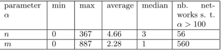
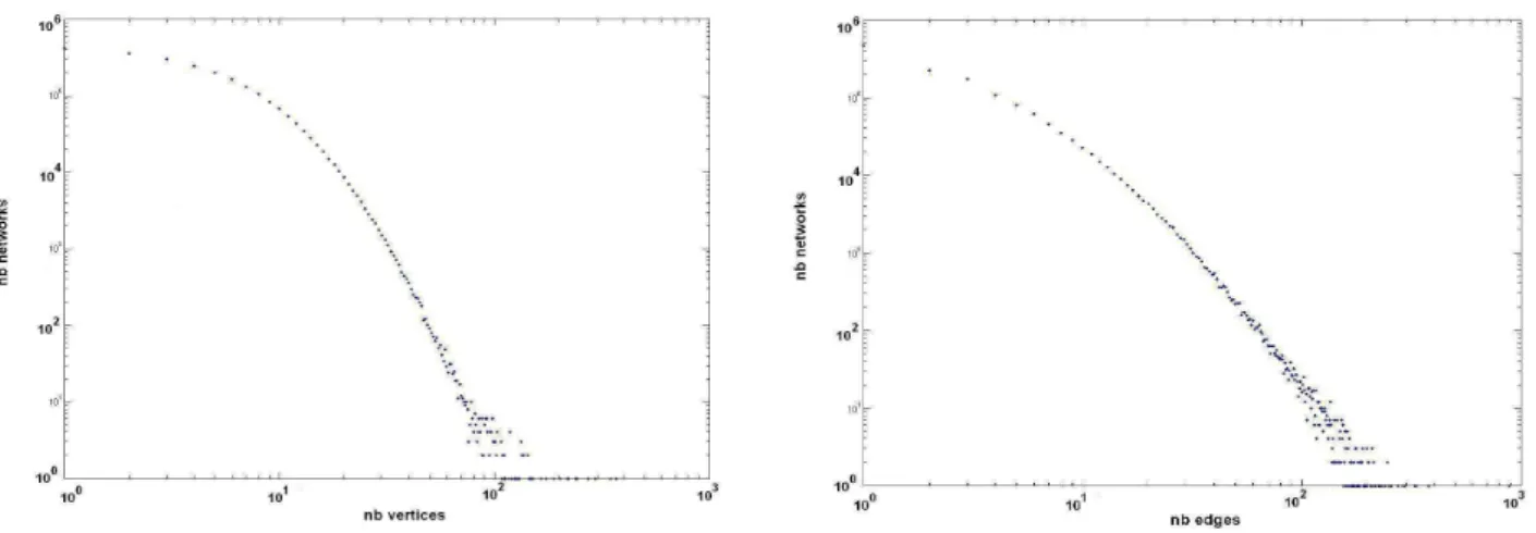
For each vertex (ego) v in GM , we study the graph Gn(v) in-duced by its neighborhood, so we analyze 2.7 × 10⁶ graphs; we denote by D = {Gn(v), v ∈ GM } this set of neighbor-hood graphs. As expected, most of these graphs have a small number of vertices (this number is equal to the degree of v) while only a small minority have a great number of ver-tices. The same statement is valid for the number of edges of each graph in D (this number is equal to the number of triangles containing ego). Table 1 contains the minimum, maximum, median and average values of the two parame-ters, as well as the number of graphs in D where the value of the parameter is greater than 100. Figure 3 contains the distribution of the number of vertices and of the number of edges of the graphs in D. Only 20 graphs (i.e. 7 × 10⁻⁴%) have more that 100 vertices and more that 100 edges. The average of the densities of the graphs in D is the clustering coefficient of GM , equal to 0.097.
Empirical complexity of the method. Let us discuss
parameter α
min max average median nb. net-works s. t. α > 100
n 0 367 4.66 3 56
m 0 887 2.28 1 560
Table 1: Different measures for the number of ver-tices (n) and the number of edges (m) of the 2.7 × 10⁶ neighborhood networks
the complexity of the method characterize when it is ap-plied to the graphs in D, i.e. when Algorithm 2 is apap-plied to the mobile phone graph GM. For a graph G in D, let nG be its number of vertices, mGits number of edges and sGits number of patterns. As we explained in the previous section, the time complexity of characterize(G) is O(sG). After ap-plying Algorithm 2 to GM , we know, for each graph G ∈ D, the number sG, so we are able to empirically determine the complexity of Algorithm 2 on GM. For all graphs G ∈ D, we have sG< m3Gand for 98.5% of these graphs sG< m2G, so, on our graph GM , the observed time complexity of the method characterize(G) is O(m2
G) in 98.5% of the cases and O(m3G) in the rest of the cases. Given that the graphs in D are not very dense, it is not very time-consuming to list all the induced subgraphs instead of just counting them. We compared the time complexity of the method proposed by Kloks et al. [20] that counts the induced subgraphs with exactly 4 vertices to that of the method proposed by Wer-nicke [36], that we use in Algorithm 1. On the one hand, for a graph G with nG vertices, the complexity of Kloks’ algorithm is O(nα
G+ e1.69), where O(n α
G) is the time needed to compute the square of the adjacency matrix of G. On the other hand, for each graph G ∈ D, the number of in-duced subgraphs with 4 vertices is smaller than (2 × mG)2 and than (5 × nG)2. Therefore, for the mobile phone graph GM, the time complexities of the two methods are compa-rable. Then it is worth listing all the subgraphs, given that we make a step further by computing not just the number of the different subgraphs but also the position classes of the vertices.
5.2
Characteristic patterns
We address here the problem of identifying the patterns that are ”characteristic” for the set D of neighborhood graphs. There are several possible definitions for a characteristic pat-tern C for a set of graphs D:
Def 1. the number of occurrences of the pattern C as in-duced subgraph of the graphs in D is greater than a given threshold;
Def 2. the number of graphs in D that contain the pattern C as induced subgraph is greater than a given thresh-old (this is the adopted approach in [17, 19, 21, 39]); Def 3. the number of occurrences of the pattern C as
in-duced subgraph is higher for the graphs in D than for randomly generated graphs of same sizes (this ap-proach was introduced in [28]).
Def 1. We computed, for each pattern C with k 6 5 ver-tices, the number of occurrences of C as induced subgraph
Figure 3: The distribution of the number of vertices (a) and of the number of edges (b) of the 2.7 × 10⁶ neighborhood networks
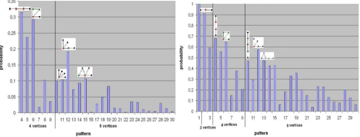
in D divided by the number of occurrences of a pattern with k vertices in D, i.e. the probability that the subgraph in-duced by k connected vertices of a graph in D represents the pattern C. Figure 4 (left) contains the values of these probability for k > 3. We observe that the patterns that oc-cur the most are the paths and the stars (possibly with an extra edge). Of course the counting of all the occurrences of a certain pattern gives an advantage to those containing vertices of degree 1.
Def 2. Figure 4 (right) contains, for each pattern C with k 6 5 vertices, the number of graphs in D that contain C as induced subgraph divided by the number of graphs in D that contain at least one pattern with k vertices, i.e. the probability that a graph in D with at least k connected ver-tices contains C. We observe that the most frequent patterns are the paths, possibly with one extra edge (added to form a star or a triangle).
Def 3. For each connected component of a graph in D we randomly generated connected graphs using the method introduced in [27]. This method computes dK−series of probability distributions (i.e. all degree correlations within d−sized subgraphs).We built graphs for d = 1, 2 and 3 re-spectively. For d = 1, the generated graphs preserve the degree distribution of the original graphs, thus assuring also the same number of vertices and edges. For d = 2, the joint degree distribution is preserved, thus keeping also the same degree distribution. For d = 3, the graph generation pre-serves the number of triangles and wedges (i.e. chains of 3 vertices connected by 2 edges) between vertices with degrees k1, k2, k3, ∀k1, k2, k3∈ N.
For each value of d, let Rd be the set of randomly gener-ated graphs. Note that all the three generations (for d = 1, 2, 3) preserve the degree and the clustering coefficient of the graph GM. For each pattern, we computed the ratio between its number of occurrences in the graphs in D and in the graphs in Rd. When the graphs in D are compared to the graphs in Rd, the patterns with the greatest values of the ratios are characteristic for the the graphs in D and the ones with the smallest values are characteristic for the
graphs in Rd. For d = 1 and d = 2, the same patterns are identified as characteristic (see Figure 5), with smaller values of the ratio for d = 2 than for d = 1. These patterns suggest that, although the densities of the input graphs are pre-served in the generated ones, there are graphs in D that are locally more dense than the corresponding generated ones. So, in the neighborhood of certain vertices, several neigh-bors form dense clusters even though they belong to the same connected component; these clusters may correspond to the different groups of contacts of that person. Note how-ever that the two generations don’t preserve the clustering coefficients of the graphs in D. When k = 3, the clustering coefficient is preserved and the observed values of the ratio are placed between 0.99 and 1.003 for all the patterns. The generated graphs essentially reconstruct the original ones, so the 3k−distribution suffices in order to capture the distribu-tions of the different patterns in the neighborhood graphs in GM. Nevertheless, this generation is very constraining for small graphs like those in D; in many cases there is only one graph that has the 3k−distribution of the original one: the original one. Besides, the structure of neighborhoods refers not only to the distributions of the different patterns, but also to the roles played by the vertices; this question is discussed in the next section.
5.3
Positions of the vertices
Recall that by applying Algorithm 2 to the graph GM we computed, for each ego v in GM and each vertex u in the neighborhood Gn(v) of v, the positions of u in Gn(v). We analyze here, for each ego v and each vertex u in Gn(v), the relation between the positions occupied by u in Gn(v) and the quantity of its communications with v. Note that the positions of u are completely determined by its links with the other vertices in Gn(v); the quantity of communication of u with ego v will also be relativized to the quantity of communication between ego and the other persons in his network.
5.3.1
The maximal number of calls
First, for each ego v, we index his neighbors depending on the number of calls they exchanged with him: the greater the number of calls exchanged with ego, the smaller the index,
Figure 4: For each pattern with k vertices, the probability: to be the subgraph induced by k connected vertices in D (left) and to occur in a graph in D that has at least k connected vertices (right)
Figure 5: For each pattern, log2 of the ratio between its nb of occurrences in D and in R2
such that the vertex with the greatest number of calls has index 1 and the one with the smallest has index d(v). Let D5 be the set of graphs in D with at least 5 vertices, i.e. the set of neighborhood graphs of the vertices in GM with degree at least 5. For each graph in D5, we study the positions occupied by its vertices with indices 1, 2, 3 and 4 and by a randomly chosen vertex between those with index greater than 4 to which we give the index 0. In order to do that, we answer two questions regarding the entire set D5:
Q1 given a position class in P5, which of the five indices occupies this position the most frequently and which one the least frequently?
Q2 given a class C ∈ C5 and an index i < 5, in which position class of C i appears the most frequently and in which one the least frequently?
For an index i < 5, let I(i) be the set of vertices that have index i in the graphs in D5 along with the corresponding
graphs: I(i) = {(u, G) s.t. u ∈ VG, G ∈ D5 and index(u) = i} . For an index i < 5 and a position class P ∈ P5, we define:
• the absolute frequency of occurrence F a(i, P ) of i in P as the total number of occurrences in P of the ver-tices with index i divided by the sum of degrees of the vertices with index i:
F a(i, P ) = P (u,G)∈I(i)P os5(G, P, u) P (u,G)∈I(i)d(u) .
• the relative frequency of occurrence F r(i, P ) of i in P as the number of graphs in D5where a vertex with in-dex i appears in the position P divided by the number of graphs in D5 where a vertex with index i has the degree at least 1 :
F r(i, P ) = | {(u, G) ∈ I(i), P os5(G, P, u) > 0} | | {(u, G) ∈ I(i), d(u) > 0} |
Question Q1. For each position class P ∈ P5, we sorted re-spectively the five values F a(i, P ) and the five values F r(i, P ), for i ∈ {0, 1, 2, 3, 4}. We find that, for most of the central position classes, the vertices with index 1 occur more often than the ones with index 2 and they occur more often than the ones with index 3 etc; the randomly selected vertices occur the least often in these central position classes. The opposite situation happens for most of the peripheral posi-tion classes, that are occupied the most frequently by the randomly chosen vertices and the least frequently by the ones with index 1. As for the intermediate positions, they are mostly occupied by the vertices with indices 3 and 4. The position classes of all the 30 isomorphism classes follow this tendency, except for those of the five following classes: 8, 21, 22, 26 and 29. Note however that in these cases the difference between central and peripheral is not very sharp and that these classes are not very frequent (see Figure 4).
Question Q2. For each isomorphism class C ∈ C5 and each index i ∈ {0, 1, 2, 3, 4} , we sorted the values F a(i, P ) of
the position classes P of C. We observe that, for all of the isomorphism classes (except 10 and 27), the vertices with index 1 occupy most frequently the central positions and least frequently the peripheral ones. The randomly chosen vertex occupies mostly the peripheral positions and least frequently the central ones, while the vertices with indices 2, 3 and 4 have a tendency placed between these two. These results allow us to make the following statement: in
most of the induced subgraphs where it appears, the person that exchanged the greatest number of calls with ego plays a central role, being a connection point between several other neighbors. The roles of the next three vertices are less cen-tral, but they remain more central than that of the randomly chosen neighbor. Note that this centrality of roles is
iden-tified using the small induced subgraphs where the vertices appear. This means that a vertex has a more or less impor-tant position with regard to the vertices that are around it and not to the whole graph. This corresponds to our aim of computing the roles of the vertices rather than measure their centrality.
5.3.2
The maximal sum of duration of calls
We analyze, for the network of each ego, the position classes occupied by the vertex that had the greatest sum of duration of calls with ego. In 78.2% of the cases, the person that exchanged the greatest number of calls with ego (the vertices with index 1 of the previous section) is also the person that has the greatest total duration. In the other cases, we gave index 1 to the vertex with the greatest number of calls and index 2 to the vertex with the greatest sum of duration of calls. We also randomly chose a vertex among the other neighbors of ego. We observe that the vertices with index 2 appear less often in a central position that the vertices with index 1 but more often that the randomly chosen vertices. The vertices with index 2 prefer the intermediate positions.
5.4
Interpretation of the results
We rely on the results of several studies in order to try to ex-plain the positions occupied by the two types of contacts of ego: the ones with the greatest frequency of calls and the one with the greatest total duration. In [25], Licoppe et Smoreda analyzed the relation between social networks, exchanges between actors and communication tools using databases of telephone calls, Internet traffic and several interviews fo-cusing on the use of telephone. For a pair of actors, they identified two patterns of relationship and the corresponding communication tools. The first pattern is that of ”connected presence”, where the two persons, socially and often also ge-ographically close, are frequently in contact with each other, exchanging many short calls and messages. They share ac-tivities that require numerous calls for synchronization and coordination, the mobile phone being especially suitable for this. In our network, the person that exchanged the greatest number of calls with ego has an important role in the net-work of neighbors, occupying central positions more often than other vertices and often connecting neighbors other-wise disconnected. The next three persons have also more important positions than a randomly selected neighbor. The second pattern identified by Licoppe et Smoreda is that of ”intermittent presence”, where the two persons, close friends or intimate relatives, are not able to see each other or talk very often. Their conversations are long, they give and
re-ceive news, trying to compensate for the rarity of face-to-face contacts. In our network, the person that has the greatest sum of duration of calls with ego, when he doesn’t have the greatest frequency too, occupies more important posi-tions than a randomly selected neighbor. It has however a less central role than the person that has the most frequent calls.
The relation between the geographical distance between two persons and the probability of existence of a link connecting them has also been studied [22, 24]. In [22], Lambiotte et al. showed that in a mobile phone network this probability is inversely proportional to the square of the geographical distance. According to [24], a similar tendency is observed in a different kind of large social networks (bloggers com-munity): the probability of existence of a link is inversely proportional to the number of closer friends. Therefore, one can imagine that in most of the neighborhoods in our mo-bile phone graph many of ego’s contacts are geographically close to him. The person that has long, but rare calls with ego probably doesn’t see him very often; it is not surprising that this person’s position is not as important as that of the contact with the greatest frequency. The duration of the calls suggests though a certain social closeness between this person and ego; he probably knows and calls some of ego’s contacts, which explains his more important position than that of a randomly chosen neighbor. Imagine, for instance, that the persons that have frequent contacts with ego are his friends or colleagues that he sees nearly daily and the person that has the greatest sum of durations is a childhood friend.
6.
CONCLUSIONS AND PERSPECTIVES
We presented in this paper a method for analyzing the local structure of large graphs that we applied to a 2.7M vertices, 6M edges mobile phone graph. In the neighborhood of each vertex (called ego) of the graph, we listed all the patterns and we identified the characteristic ones. Then we addressed the notion of role in a graph, focusing on the position occu-pied by each vertex and the importance of this position. Our goal was not to define a certain centrality of the vertices, but rather to find how they connect to each other, how they are placed and how important they are in the local structures they form with the other vertices.
A step further could be to compare neighborhood graphs for instance by merging vertices having ”similar” functions. We believe indeed that the identification of patterns and positions of vertices can offer the context for new definitions of similarity. We hope that future research based on the notions introduced in this paper will provide new methods for measuring the similarity between graphs and between roles of vertices. It would also be interesting to apply this method to another kind of large graphs, for instance to on-line communities where the neighborhoods are more dense but the connections between people are weaker.
7.
REFERENCES
[1] R. Agrawal and R. Srikant. Fast algorithms for mining association rules in large databases. In VLDB ’94. [2] A.-L. Barabasi and R. Albert. Emergence of scaling in
[3] F. Barth. Political leadership among the Swat
Pathans. Athlone Press, London, 1959.
[4] J. Boissevain. Friends of Friends, Networks,
Manipulators and Coalitions. Basil Blackwell, Oxford,
1974.
[5] S. Borgatti and M. Everett. The class of all regular equivalences: Algebraic structure and computation.
Social Networks, 11(1):65–88, March 1989.
[6] S. Bornholdt and H. G. Schuster, editors. Handbook of
Graphs and Networks. Wiley-Vch, 2003.
[7] E. Bott. Family and Social Network. Tavistock, London, 1957.
[8] R. Breiger, S. Boorman, and P. Arabie. An algorithm for clustering relational data with applications to social network analysis and comparison with multidimensional scaling. Journal of Mathematical
Psychology, 12:328–383, 1975.
[9] S. Brin and L. Page. The anatomy of a large-scale hypertextual Web search engine. Computer Networks
and ISDN Systems, 30(1–7):107–117, 1998.
[10] J. Candia, M. C. Gonz´alez, P. Wang, T. Schoenharl, G. Madey, and A. Barab´asi. Uncovering individual and collective human dynamics from mobile phone records. Journal of Physics A: Mathematical and
Theoretical, 41(6):224015+, June 2008.
[11] K. Efe, V. Raghavan, C. H. Chu, A. L. Broadwater, L. Bolelli, and S. Ertekin. The shape of the Web and its implications for searching the Web, 2000.
[12] G. Flake, S. Lawrence, and C. L. Giles. Efficient identification of web communities. In Sixth ACM
SIGKDD International Conference on Knowledge Discovery and Data Mining, pages 150–160, Boston,
MA, 2000.
[13] L. Freeman. A set of measures of centrality based on betweenness. Sociometry, 40:35–41, 1977.
[14] D. Gibson, J. M. Kleinberg, and P. Raghavan. Inferring web communities from link topology. In
ACM Conference on Hypertext and Hypermedia, pages
225–234, 1998.
[15] J. Han, J. Pei, and Y. Yin. Mining frequent patterns without candidate generation. SIGMOD Rec., 29(2):1–12, 2000.
[16] C. Haythornthwaite. Social networks and internet connectivity effects. Information, Communication and
Society, 8(2):125–147, June 2005.
[17] H. He and A. Singh. Graphrank: Statistical modeling and mining of significant subgraphs in the feature space. In ICDM ’06.
[18] B. Hogan. The Handbook of Online Research Methods, chapter Analyzing Social Networks via the Internet. Sage: Thousand Oaks, CA, 2008.
[19] A. Inokuchi, T. Washio, and H. Motoda. An apriori-based algorithm for mining frequent substructures from graph data. In PKDD ’00. [20] T. Kloks, D. Kratsch, and H. M¨uller. Finding and
counting small induced subgraphs efficiently.
Information Processing Letters, 74(3-4):115–121, 2000.
[21] M. Kuramochi and G. Karypis. Frequent subgraph discovery. In ICDM ’01.
[22] R. Lambiotte, V. Blondel, C. de Kerchove, E. Huens, C. Prieur, Z. Smoreda, and P. V. Dooren.
Geographical dispersal of mobile communication networks. Physica A, 387(21):5317–5325, September 2008.
[23] M. Latapy. Main-memory triangle computations for very large (sparse (power-law)) graphs. Theoretical
Computer Science (TCS), (407):458–473, 2008.
[24] D. Liben-Nowell, J. Novak, R. Kumar, P. Raghavan, and A. Tomkins. Geographic routing in social networks. Proceedings of the National Academy of
Sciences, 102(33):11623–11628, August 2005.
[25] C. Licoppe and Z. Smoreda. Are social networks technologically embedded? how networks are changing today with changes in communication technology.
Social Networks, 27(4):317–335, October 2005.
[26] F. Lorrain and H. White. Structural equivalence of individuals in social networks. Journal of
Mathematical Sociology, 1:49–80, 1971.
[27] P. Mahadevan, D. Krioukov, K. Fall, and A. Vahdat. Systematic topology analysis and generation using degree correlations. SIGCOMM Comput. Commun.
Rev., 36(4):135–146, 2006.
[28] R. Milo, S. Shen-Orr, S. Itzkovitz, N. Kashtan, D. Chklovskii, and U. Alon. Network motifs: Simple building blocks of complex networks. Science, 298(5594):824–827, October 2002.
[29] M. E. J. Newman. The structure and function of complex networks. SIAM Review, 167(45), 2003. [30] J. P. Onnela, J. Saram¨aki, J. Hyv¨onen, G. Szab´o,
D. Lazer, K. Kaski, J. Kert´esz, and A. L. Barab´asi. Structure and tie strengths in mobile communication networks. Proceedings of the National Academy of
Sciences, 104(18):7332–7336, May 2007.
[31] C. Prieur, A. Stoica, and Z. Smoreda. Extraction de r´eseaux ´egocentr´es dans un (tr`es grand) r´eseau social.
Bull. de M´ethodologie Sociol., (101), 2009.
[32] J. Scott. Social Network Analysis. Sage, London, 1992. [33] S. Wasserman and K. Faust. Social Network Analysis:
Methods and Applications. Cambridge University
Press, 1994.
[34] D. Watts and S. Strogatz. Collective dynamics of small-world networks. Nature, 393, 1998.
[35] B. Wellman. An egocentric network tale. Social
Networks, 15:423–436, 1993.
[36] S. Wernicke. Efficient detection of network motifs.
IEEE/ACM Trans. Comput. Biol. Bioinformatics,
3(4):347–359, 2006.
[37] H. White, S. Boorman, and R. Breiger. Social structure for multiple networks i. blockmodels of roles and positions. American Journal of Sociology, 81, 1976.
[38] X. Yan, H. Cheng, J. Han, and P. Yu. Mining
significant graph patterns by leap search. In SIGMOD
’08.
[39] X. Yan and J. Han. gspan: Graph-based substructure pattern mining. In ICDM ’02.