HAL Id: insu-01017024
https://hal-insu.archives-ouvertes.fr/insu-01017024
Submitted on 2 Jul 2014HAL is a multi-disciplinary open access
archive for the deposit and dissemination of sci-entific research documents, whether they are pub-lished or not. The documents may come from teaching and research institutions in France or abroad, or from public or private research centers.
L’archive ouverte pluridisciplinaire HAL, est destinée au dépôt et à la diffusion de documents scientifiques de niveau recherche, publiés ou non, émanant des établissements d’enseignement et de recherche français ou étrangers, des laboratoires publics ou privés.
Modeling the effect of soil structure on water flow and
isoproturon dynamics in an agricultural field receiving
repeated urban waste compost application
Vilim Filipović, Yves Coquet, Valerie Pot-Genty, Sabine Houot, Pierre Benoit
To cite this version:
Vilim Filipović, Yves Coquet, Valerie Pot-Genty, Sabine Houot, Pierre Benoit. Modeling the effect of soil structure on water flow and isoproturon dynamics in an agricultural field receiving repeated urban waste compost application. Science of the Total Environment, Elsevier, 2014, 499, pp.546-559. �10.1016/j.scitotenv.2014.06.010�. �insu-01017024�
Modeling the effect of soil structure on water flow and isoproturon dynamics in an agricultural field receiving repeated urban waste compost application
Vilim Filipović1,2,3
, Yves Coquet2, Valérie Pot3, Sabine Houot3, Pierre Benoit3
1Department of Soil Amelioration, Faculty of Agriculture, University of Zagreb, Svetošimunska 25,
10000 Zagreb, Croatia, e-mail: vfilipovic@agr.hr
2Université d’Orléans, ISTO, UMR 7327, 45071, Orléans, France ; CNRS/INSU, ISTO, UMR 7327,
45071 Orléans, France ; BRGM, ISTO, UMR 7327, BP 36009, 45060 Orléans, France
3
INRA, AgroParisTech , UMR 1091 EGC, F-78850 Thiverval-Grignon, France
Abstract
Transport processes in soils are strongly affected by heterogeneity of soil hydraulic properties. Tillage practices and compost amendments can modify soil structure and create heterogeneity at the local scale within agricultural fields. The long term field experiment QualiAgro (INRA-Veolia partnership 1998-2013) explores the impact of heterogeneity in soil structure created by tillage practices and compost application on transport processes. A modeling study was performed to evaluate how the presence of heterogeneity due to soil tillage and compost application affects water flow and pesticide dynamics in soil during a long term period. The study was done on a plot receiving a co-compost of green wastes and sewage sludge (SGW) applied once every two years since 1998. The plot was cultivated with a biannual rotation of winter wheat-maize (except one year of barley) and a four-furrow moldboard plough was used for tillage. In each plot, wick lysimeter outflow and TDR probes data were collected at different depths from 2004, while tensiometer measurements were also conducted during 2007/2008. Isoproturon concentration was measured in lysimeter outflow since 2004. Detailed profile description was used to locate different soil structures in the profile, which was then implemented in the HYDRUS-2D model. Four zones were identified in the ploughed layer: compacted clods with no visible macropores (Δ), non-compacted soil with visible macroporosity (Γ),
interfurrows created by moldboard ploughing containing crop residues and applied compost (IF), and the plough pan (PP) created by ploughing repeatedly to the same depth. Isoproturon retention and degradation parameters were estimated from laboratory batch sorption and incubation experiments, respectively, for each structure independently. Water retention parameters were estimated from pressure plate laboratory measurements and hydraulic conductivity parameters were obtained from field tension infiltrometer experiments. Soil hydraulic properties were optimized on one calibration year (2007/08) using pressure head, water content and lysimeter outflow data, and then tested on the whole 2004/2010 period. Lysimeter outflow and water content dynamics in the soil profile were correctly described for the whole period (model efficiency coefficient: 0.99) after some correction of LAI estimates for wheat (2005/06) and barley (2006/07). Using laboratory-measured degradation rates and assuming degradation only in the liquid phase caused large overestimation of simulated isoproturon losses in lysimeter outflow. A proper order of magnitude of isoproturon losses was obtained after considering that degradation occurred in solid (sorbed) phase at a rate 75% of that in liquid phase. Isoproturon concentrations were found to be highly sensitive to degradation rates. Neither the laboratory-measured isoproturon fate parameters nor the independently-derived soil hydraulic parameters could describe the actual multiannual field dynamics of water and isoproturon without calibration. However, once calibrated on a limited period of time (9 months), HYDRUS-2D was able to simulate the whole 6-year time series with good accuracy.
Highlights
Impact of soil heterogeneity on water flow and isoproturon dynamics was evaluated.
Soil heterogeneity was created by moldboard ploughing and compost amendments.
A longterm numerical modeling on field experiment was performed using HYDRUS-2D.
HYDRUS-2D described accurately lysimeter outflows and IPU loss after calibration.
S
oil structures in tilled layer (Γ,Δ, IF) had a large influence on IPU distribution.
1. Introduction
Water flow and contaminant transport in the vadoze zone can be strongly affected by soil structure heterogeneity. Soil structure can be defined as the arrangement of solid and void space that exists in a soil at a given time (Kay, 1990). Its heterogeneity can be caused by natural processes or by anthropogenic interventions like soil tillage, fertilization or compost application. Soil tillage has a very important influence on soil structure and thus on soil hydraulic properties. Tillage practices may include a wide range of agricultural operations, ranging from reduced tillage or no-till practices in conservation systems to moldboard ploughing as in conventional systems. Soil tillage and management affect soil hydraulic properties with consequences for the storage and movement of water, nutrients and pollutants, and for crop growth (Strudley et al., 2008). It can cause changes in soil pore-size distribution and in saturated hydraulic conductivity (Coutadeur et al., 2002; Mubarak et al., 2009; Or et al., 2000; Xu and Mermoud, 2003) and hence influence water flow pathways and solute transport in soil. Conventional tillage generally reduces solute preferential transport by disrupting functional macropores (Jarvis, 2007), as suggested in the studies by Javaux et al. (2006) and Vanclooster et al. (2005). Tillage can generate heterogeneities within the soil profile, and may produce various compacted and non-compacted zones or clods (Manichon and Roger-Estrade 1990). Compacted zones generally have a much lower hydraulic conductivity than non-compacted zones (Ankeny et al., 1990; Schneider et al., 2009) and may have a large influence on water flow and solute
transport. Coquet et al. (2005a) performed a field experiment to explore the impact of soil structure heterogeneity created by agricultural operations (trafficking, ploughing) on water flow and solute transport. Water and solute transport were mostly associated with non-compacted soil, while very little water or bromide penetrated compacted clods thus engaging preferential (funneled) flow patterns around them.
In addition to soil tillage, application of organic amendments into soil can alter soil structure and thus have an effect on water flow and solute dynamics. Compost amendment to soil increases soil organic matter content and has an effect on pesticide sorption and degradation (De Wilde et al., 2008; Guo et al., 1993; Kodešová et al., 2011). Organic matter increases macroporosity and infiltration rates, but can lead to a decrease of hydraulic conductivity at low pressure head (Gupta et al., 1977). Schneider et al. (2009) performed a study on the effect of urban waste compost incorporation on near saturated hydraulic conductivity. They found that the large variability of soil hydraulic conductivity within the tilled layer was predominantly controlled by tillage practices rather than by compost amendments. Pot et al. (2011) quantified the effects of tillage practice and repeated compost application on isoproturon transport in a tilled layer using column leaching experiments. While hydraulic conductivity measurements showed that tillage practice had a major effect compared to compost application, column leaching experiments showed no statistically significant effect of either tillage practice or compost addition.
Numerical models have been used to explain water flow and pesticide behavior in soil (Dousset et al., 2007; Kodešová et al., 2005; Pot et al., 2005). Gärdenäs et al. (2006) compared four conceptually different preferential flow and/or transport approaches for their ability to simulate drainage and pesticide leaching to tile drains.Model predictions were compared against drainage and MCPA concentration measurements made in a tile-drained field in southern Sweden. Authors concluded that two-dimensional models are suitable tools for studying pesticide leaching from tile-drained fields with large spatial variability in soil properties. Coquet et al. (2005b) used the numerical model HYDRUS-2D to successfully reproduce water flow and bromide transport in a soil profile that contained compacted and non-compacted soil zones. After minor adjustments of the van Genuchten
soil hydraulic parameters α and Ks, the model reproduced water and bromide dynamics quite well. The work presented here goes one step further using the same approach but on the long term (six years) to model water and isoproturon dynamics in a heterogeneous soil profile.
Isoproturon [3-(4-isopropylphenyl)-1,1-dimethylurea] is frequently used to control weeds in cereal crops and is one of the most detected herbicides in surface and ground waters, especially in France (SOeS, 2012). For this reason, isoproturon dynamics in soil has been largely studied in laboratory and field experiments. Dousset et al. (2007) performed displacement experiments of isoproturon in disturbed and undisturbed soil columns of a silty loam soil under similar rainfall intensities. Köhne et al. (2006) studied the physical and chemical nonequilibrium processes governing isoproturon transport under variably saturated flow conditions in undisturbed soil columns. Pot et al. (2005) also performed displacement experiments with isoproturon on two undisturbed grassed filter strip soil cores under unsaturated steady state conditions. Column leaching experiments are very useful for studying the coupling between pesticide transport, sorption and degradation processes, but they can hardly be multiplied in large number or performed at a large scale, so it is difficult to account for the spatial heterogeneity of the tilled layer at the plot scale with such a technique. One way to account for the spatial heterogeneity of the tilled layer is to use two- or three- dimensional transport models which allow accounting explicitly for the spatial distribution of the different soil structures encountered in the tilled layer at the plot scale. Meanwhile, pesticide modeling allows combining complex processes such as water flow, solute transport, heat transport, pesticide sorption, transformation and degradation, volatilization, crop uptake or surface runoff.
In this paper, we attempted to model a long term field experiment, which was carried out on an agricultural field receiving repeated urban waste compost applications. Wick lysimeters were used to quantify water flow and isoproturon leaching. The main objective of this work was to evaluate how the presence of different soil structures in the tilled layer (due to soil tillage and compost application) affects water flow and isoproturon dynamics during a multiannual (six years) time period. In this paper, we explicitly account for soil heterogeneity created by tillage and compost addition using a two-dimensional model for describing water flow and isoproturon transport in soil.
2. Materials and methods 2.1. Field experiment
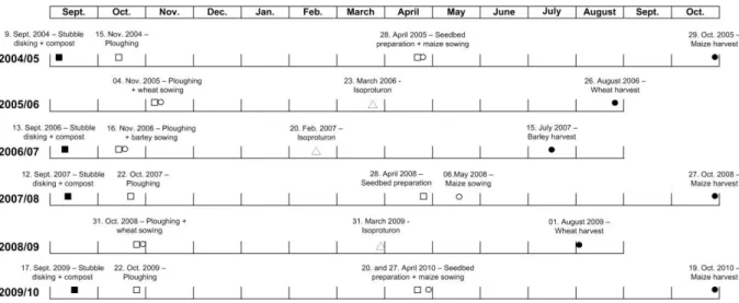
The experimental field site was located at Feucherolles (Yvelines, France) in the western part of the Parisian Basin. The soil was a silt loam Albeluvisol (WRB), and contained on average 19% clay, 75% silt, and 6% sand in the ploughed layer. The soil profile was composed of five horizons: a tilled loamy LA horizon (0-28 cm), an eluviated silt loam E horizon (38-50 cm), an illuviated silty clay loam BT horizon (50-90 cm), a transition silty clay loam BT/IC horizon (90-145 cm), and a silty loam structure-less decarbonated loess IC horizon (145-200 cm). A field experiment was designed to evaluate the effects of urban waste compost application to soil since 1998. The field has been cultivated with a biannual rotation of winter wheat (Triticum spp.) and maize (Zea mays L.) (Fig. 1), except in 2006/07 when barley (Hordeum vulgare L.) was grown due to corn rootworm (Diabrotica
virgifera virgifera Leconte) infestation in the area. Urban waste compost was applied over wheat or
barley stubble and secondary tillage (stubble disking) was immediately carried out to incorporate composts and straws within the upper soil layer (25 cm). The soil was ploughed once every year in October or November to a depth of 28 cm with a four-furrow moldboard plough (ploughing width 40 cm). In spring 2005, 2008 and 2010, seed bed was prepared for maize sowing using a tined cultivator. Each compost application was conducted every two years (a supplementary compost application was made in September 2007 on barley) and was applied in an amount of four tons of organic carbon per ha. The application of isoproturon was performed three times (Fig. 1) during 2004/2010 at the rate of 1000 g per ha. One plot receiving a co-compost of sewage sludge and green wastes (SGW) was selected for this modeling study. Since 1998, the repeated compost applications have increased soil organic C content by about 10% compared with the control plot (Houot et al., 2009; Schneider et al., 2009).
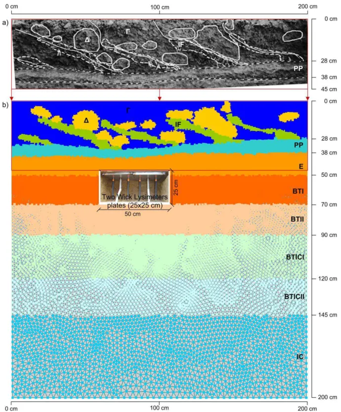
Soil structure in the tilled layer was described in December 2004 according to Manichon’s (1982) method, which is based on the visual observation of soil macroscopic features on the vertical face of a large soil pit dug perpendicular to the tillage direction (Coutadeur et al., 2002; Roger-Estrade et al., 2000). The profile (45 cm deep and 2 m wide) was divided into vertical and horizontal compartments according to the effects of tillage practices, and a description of the internal structures of each of these compartments was made. Three soil zones were distinguished in the tilled layer (Fig. 2):
- Furrows – bands of soil which have been cut and rotated by the moldboard plough – are composed of zones with compacted Δ structure and zones with Γ macroporous structure. The Δ structure has smoothly breaking faces and no structural porosity, and is characteristic of compacted soil zones. It may be found under recent wheel tracks or in clods located in the ploughed layer between the wheel tracks and created by the ploughing that cut and fragmented the compacted soil formed under former wheel tracks. The Γ structure is formed by the coalescence of macroporous aggregates or clods, with clearly visible structural porosity. - Interfurrows (IF) – formed between the furrows created by the moldboard plough. They
contain a large amount of organic matter originating from the plant residues of the preceding crop and/or from recent compost application. It is characterized by structural porosity clearly visible by eye and large amounts of organic residues.
- An additional layer corresponding to a plough pan (PP) was distinguished between the tilled layer and underlaying untilled E horizon from ~ 28 to 38 cm. This plough pan, characterized by a continuous Δ structure, is result of the long term ploughing of the soil to the same depth.
2.3. Soil hydraulic properties
Near-saturated soil hydraulic conductivity was calculated from infiltration rates measured for each type of soil structure using a disc tension infiltrometer with a 4 cm-diameter base (Schneider et al., 2009). The 4 cm-diam. base size was chosen because of the small lateral dimensions of some of the soil zones to be characterized (e.g., interfurrows). Steady-state infiltration rates were measured at
five soil water potentials: –0.6, –0.4, –0.2, –0.125 and –0.05 kPa. The hydraulic conductivity was calculated from the steady-state infiltration rates in accordance to the multipotential technique (Reynolds and Elrick, 1991). Saturated hydraulic conductivity was extrapolated from the [–0.2, –0.05 kPa] interval assuming a K-h exponential relationship. Water retention values were measured in the laboratory for each structure using Richards’ pressure plate (Klute and Dirksen, 1986). Samples with a volume of 50 cm3 (2.55 cm height and 5 cm diameter) were taken from the soil when soil water content was close to field capacity. Applied pressure heads were: -1, -3, -10, -30, -100, -310, -1000 and -1580 kPa, successively. The θr, α, and n parameters of the soil water retention curve were optimized using the RETC software (van Genuchten et al., 1991) by fitting the measured retention and hydraulic conductivity data. A relative weight of 0.1 for hydraulic conductivity against retention was selected. R2 values varied from 0.81 to 0.99. Average bulk density profiles were measured using three 500 cm3 soil cores (9 cm by 8.4-cm diameter) taken from each soil horizon in November 2007.
2.4. Field monitoring
Water content was measured in the field using TDR (Trase system) probes (rod length 20 cm) which were installed at the 20, 40, 60, 80, and 100 cm depths. The TDR system was operating during the whole research period (2004-2010). Gravimetric water contents were measured on soil samples taken with an auger at multiple dates during the 2007/2008 agricultural year and used for TDR probe calibration. In addition, pressure head values were measured using tensiometers which were installed at 20, 40, 60, 80, 100, 130, and 160 cm depth during 2007/08. The tensiometers had 7.5-cm-long, 9.9-mm-diameter ceramic ends mounted on 40-cm (for the tensiometers at the 20-cm depth) or 55-cm PVC tubes connected to pressure manometers. Daily weather data was recorded at a meteorological station located 500 m from the field experiment. Data included rainfall, air temperature, air humidity, wind speed, and net radiation. Two passive capillary-wick lysimeters (25 cm x 25 cm) were installed within the plot at 45 cm depth one beside each other (Fig. 2). The depth of 45 cm was selected in order to install the lysimeter as close as possible to the ploughed layer (where the major heterogeneities were located) while still allowing for normal agricultural practices. Fiberglass wicks (Peperell, ½ inch) were
untwisted and mounted on a stainless steel plate that was installed horizontally under the undisturbed soil. The fiberglass wick does not only provide the suction, but simultaneously serves as a sampling device through which leachate was collected towards a 10 L tank buried in the soil at the depth of 1.20 m. The fiberglass wick was inserted in a Tygon tube, and had a length of 70 cm, which corresponds to a pressure head of -70 cm applied to the above-laying soil. Prior to installation, the fiberglass wicks were placed in a muffle oven for 4 hours at 400 ˚C to remove organic impurities (Knutson and Selker, 1993). Batch experiments were performed in the laboratory using the whole sampling device (stainless steel plate, fiberwick and tygon tubes) to detect any sorption of isoproturon, and did not show any significant amount of sorption (data not shown). Water was collected through the wick lysimeters and samples were filtered at 0.45 μm and stored at 4˚C before analysis. Isoproturon concentrations were measured by the Institut Pasteur (Lille, France) using online SPE-LC-MS-MS (QUATTRO Premium 2005) and following NF EN ISO 11369. The quantification limit was 0.02 μg l−1 for isoproturon.
2.5. Isoproturon fate parameters
Sorption coefficients Kd of isoproturon were measured by Pot et al. (2011) for each morphological zone (Γ, Δ, IF, PP) in batch with 14C-isoproturon solution prepared at 0.51 mg l−1 in calcium chloride (0.01 M). Sorption isotherms obtained with the same soil in a concentration range of 0.01 to 1 mg l−1 were characterized by Freundlich exponent coefficients (n) close to 0.96 and R2 = 0.99. For the subsoil (E, BT, BTIC, IC), Kd values were obtained using the same procedure but with a lower isoproturon concentration (0.10 mg l−1) assuming that concentrations reaching horizons below the ploughed layer were lower than in the topsoil (Simon, 2012). Samples were taken from the same soil pit based on a precise description of the soil profile, then sieved at 2 mm and air-dried. Soil suspensions were prepared in glass centrifuge tubes with three grams of soil dispersed in 10 mL 14 C-isoproturon solution.After 24h of equilibrium obtained by end-over-head shaking, the supernatant was recovered by centrifugation and its radioactivity was measured allowing for the calculation of the
sorbed concentration (se in mg kg
-1
). The sorption coefficient relating the sorbed concentration of solute on soil particles, s, to the solute concentration in solution, c, is calculated as:
(1)
where ce (in mg l
-1
) is the solution concentration after 24 h equilibrium.
In January and May 2005, 14C-isoproturon mineralization was followed under laboratory controlled conditions (28 ˚C, 80% of water content at pF = 2.5) during 65 days. Fresh soil samples from each zone (15 g dry weight equivalent) were sprayed with an aqueous solution of 14C isoproturon at 12 mg l-1 corresponding approximately to the agronomic dose of 1.1 kg ha-1. Three replicates per zone were performed. The evolved 14C–CO2 was trapped in 5 ml of 1 N NaOH solutions that were
changed after 3, 7, 16, 24, 30, 42, 51, 60 and 65 days of incubation. Trapping solutions were analysed for 14C–CO2 concentrations by adding 10 ml of scintillating liquid (Ultima Gold XR Packard) and
counting 10 min in a Tri-Carb 2100TR scintillation counter (Perkin Elmer Ins., Courtaboeuf, France). More details about the degradation study can be found in Vieublé-Gonod et al. (2009).
2.6. Modeling
2.6.1. Water flow and solute transport equations
Water flow and isoproturon transport simulations were carried out using the HYDRUS-2D software (Šimůnek et al., 2008) that numerically predicts two-dimensional water flow and solute transport in variably saturated porous media. Water flow is solved using Richards’ equation:
(2)
where θ represents volumetric water content [L3 L-3], h is pressure head [L], xi (i=1, 2) are the spatial coordinates [L], t is time [T], are the components of the dimensionless anisotropy tensor (KA) in
the two main spatial direction (x, z), K is the unsaturated hydraulic conductivity [L T-1], S represents a sink term (root water uptake).
Solute transport is modeled using the advection-dispersion equation assuming first order degradation kinetics of the solute in the liquid and solid phases and an instantaneous and linear sorption of the solute onto soil solid surfaces (from Eq. 1):
(3)
where c is the solute concentration in the liquid phase [M L-3], s is the solute concentration in the solid
phase [M M-1], b is the soil bulk density [M L -3
], is the ith component of the volumetric water flux
density [L T-1], are the components of the dispersion coefficient tensor [L2 T-1], μl is the first-order
degradation rate in the liquid phase [T−1], μs is the first-order degradation rate in the solid phase [T−1],
and R is the retardation factor [-], written:
(4).
Degradation was assumed to be depended on temperature and water content. Dependence on soil water content was assumed to follow Walker’s equation (Walker, 1974):
[ ] (5)
where μr and μ are the degradation rates being considered at a reference water content, θref, and at the actual water content, θ, respectively; and b is Walker’s exponent. The temperature dependency of the isoproturon degradation rate was expressed by the Arrhenius equation (Stumm and Morgan, 1981), which can be written:
( ) (6)
where μT and μr are the values of the degradation rate at a reference absolute temperature Tr A
and actual absolute temperature TA, respectively; Ru is the universal gas constant, and Ea (J mol
-1
) is the activation energy.
Soil hydraulic functions θ(h) and K(h) were described using the van Genuchten-Mualem model (van Genuchten, 1980), which is defined as follows:
| | (7)
(8)
(9)
1 (10)
where θr and θs denote residual and saturated volumetric water content [L 3
L-3], respectively, Ks is the saturated hydraulic conductivity [L T-1], Se is the effective saturation, α [L
-1
], and n [-] are shape parameters, and l is a pore connectivity parameter. The pore connectivity parameter was taken from an average value for many soils (l=0.5) (Mualem, 1976). A modified van Genuchten (1980) model with an air-entry value of 2 cm was used in all simulations. This modification is a very minor change in the shape of the water retention curve near saturation, but significantly affects and improves predictions of the hydraulic conductivity function near saturation, especially for fine textured soils with small n values (Vogel et al., 2001).
2.6.2. Simulation domain, initial and boundary conditions
Simulations were performed on two-dimensional rectangular domain 200 cm wide and 200 cm deep (Fig. 2b). The time period for simulations was from 1 November 2004 until 27 October 2010, split into ten separate simulations (there is no option for crop rotation in HYDRUS-2D, therefore each crop or bare soil period was simulated separately) which were connected sequentially by assigning the final pressure head, temperature, and concentration distribution from the preceding simulation as initial condition for the next one. The material distribution was selected according to the field description of the soil profile in which the different structures (Γ, Δ, IF) and layers (PP, E, BT, BTIC, IC) were distinguished (Fig. 2b). The initial condition for water content was set as a hydrostatic pressure head distribution with -100 cm at the bottom of soil profile. Initial solute (isoproturon) concentration in the whole soil profile was set to zero (the measured concentration in lysimeter outflow was zero at the beginning of the experiment). An atmospheric boundary condition was selected at the top of the soil profile and free drainage boundary condition was selected at the bottom. A seepage face boundary condition with suction (pressure head of -70 cm) was implemented to represent the wick lysimeters.
HYDRUS-2D allows specifying only one seepage face. Thus, the outflow measurements of the two lysimeters were summed up according to one 50 cm long and 25 cm wide lysimeter plate. Third type solute boundary conditions were selected for isoproturon transport, at top, bottom and lysimeter plate boundaries. Water extraction by roots was simulated using Feddes model (Feddes et al., 1978) with different parameter sets for maize, wheat and barley, respectively, assuming a linear root density distribution according to depth from a maximum root density at the surface down to zero at the maximum rooting depth. Maximum rooting depth was 110 cm for maize and 140 cm for wheat and barley. The root water uptake parameters were selected from the HYDRUS database i.e. according to Wesseling (1991). LAI and crop growth parameters (crop height and rooting depth) were derived from the STICS model (Brisson et al., 2002) and were used as input parameters for HYDRUS-1D for potential evaporation and transpiration rates calculation according to the Penman-Monteith approach (Monteith, 1981). Molecular diffusion coefficient of isoproturon (0.0179 cm2 h-1) was taken from Jury et al. (1983). Longitudinal dispersivity DL was taken from Chalhoub et al. (2013), while transverse dispersivity DT was assumed to be one fifth of DL. Isoproturon sorption properties were taken from studies performed earlier on the same field (Pot et al., 2011; Simon, 2012). Isoproturon degradation rate in the liquid phase μl was calculated from the incubation experiments of Vieublé-Gonod et al.
(2009) assuming that degradation took place only in the liquid phase. Walker’s coefficient b and energy of activation Ea were taken from Cheviron and Coquet (2009). Soil parameters that varied according to depth or type of soil structure are presented in Table 1. Model efficiency coefficient E (Nash and Sutcliffe, 1970) was used to assess the level of agreement between predicted and observed data. To quantify the sensitivity of IPU loss to degradation rates, a ratio of variation (ROV) was calculated according to (Dubus et al., 2003):
(11)
where O represents the value of the output variable (IPU loss), OBC represents its value in the base-case scenario, I is the value of the input parameter (degradation rate), and IBC is its value in the base-case scenario.
3. Results and discussion 3.1. Water flow
A first set of simulations was performed using the independently measured soil hydraulic parameters obtained from laboratory water retention and field hydraulic conductivity measurements (Table 1). The main differences between the layers can be seen in the values of saturated hydraulic conductivity, which varied from 12.8 for the plough pan (PP) to 353 cm day-1 for the interfurrows (IF). Large differences in saturated hydraulic conductivity can be noticed within the tilled layer between compacted (Δ) and non-compacted (Γ) soil. After a first run for the entire simulation period, no outflow was simulated in the lysimeter, i.e. independently measured soil hydraulic parameters were not able to describe field outflow measurements. The large value of saturated hydraulic conductivity (82.3 cm day-1) of the E horizon (38-50 cm), in which the plates were located, caused the bypass of water around the lysimeters toward the deeper layers. The calibration of soil hydraulic properties was then performed based on water content, pressure head and lysimeter outflow data measured in 2008. The calibration was first tried using the inverse numerical procedure implemented in HYDRUS-2D (Hopmans et al., 2002). The calibration was performed on a time period from 24 January to 27 October 2008 (9 months) with maize grown from 06 May until the end of the calibration period. This period was selected because of the large data set available and the fact that the lysimeter outflow was collected the day before beginning the simulation. The initial pressure head distribution was set up according to the tensiometer measurements (-61 cm at 20 cm depth; -40 cm at 40; -36 cm at 60; -29 cm at 80; -25 cm at 100; -41 cm at 130; -40 cm at 160 cm depth). However, due to the complexity of the two-dimensional simulation domain and the large number of soil parameters, the inverse numerical procedure was not able to give a realistic set of soil hydraulic parameters.
Manual calibration was then performed against the field TDR, tensiometers and cumulative lysimeter outflow measurements simultaneously as stated before. At the start of the calibration process, the number of soil layers was increased in order to match the number of measurement depths i.e. 10 materials for 8 layers (Table 2). For the calibration, only one soil material (Γ structure) was
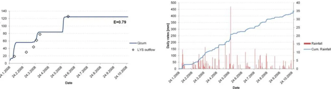
considered to compose the entire tilled layer since only one TDR probe and tensiometer were installed in that layer. The Γ structure was selected because it occupies the largest part of the tilled layer (835.4 cm2) compared to the Δ (312.9 cm2) and IF (258.8 cm2) structures. After having significantly decreased the saturated hydraulic conductivity in each layer (Table 2), the model was able to fit the cumulative lysimeter outflow data with good accuracy (E=0.79) (Fig. 3). The model reacted well to high intensity rainfalls and generated large amounts of outflow.
The volumetric water content (TDR) and pressure head (TEN) measurements were fitted reasonably well after adjustments of the saturated hydraulic conductivities and the van Genuchten’s α and n shape parameters (Table 2, Fig. 4). Model efficiency coefficients varied from 0.50 to 0.92 and from 0.05 to 0.87 for volumetric water content and pressured head measurements, respectively. A simulation was performed including Δ and IF structures in the tilled layer for the calibration period. Introducing Δ and IF structures did not affect the model efficiency (E=0.79) of the cumulative outflow results. There were small changes in E values for TDR (max ΔE=0.03) and TEN data (max ΔE=0.1) depending on depth.
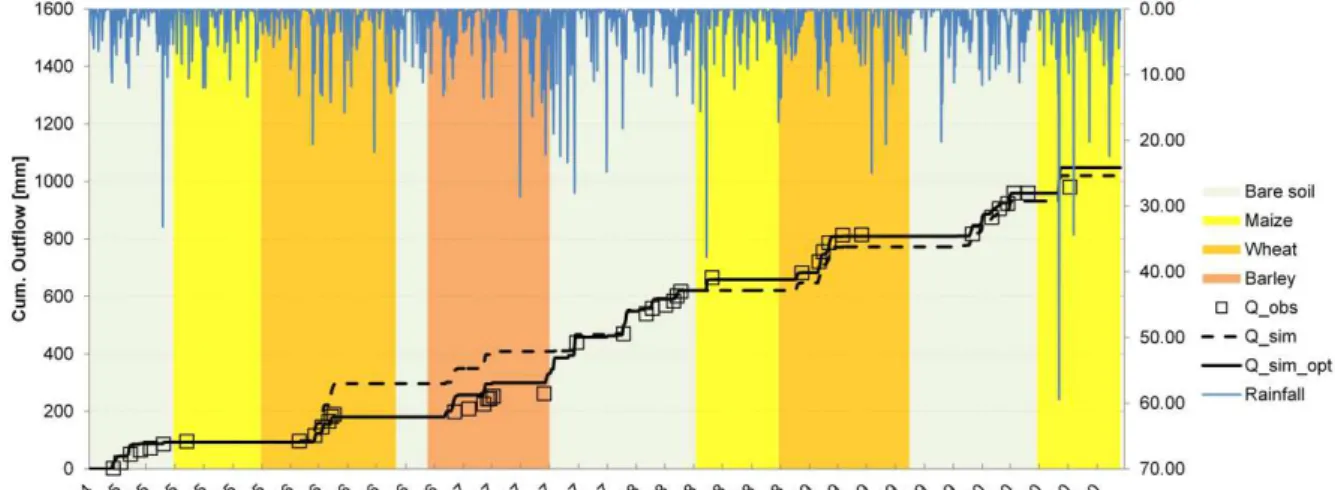
After calibration of the soil hydraulic properties, HYDRUS-2D was able to simulate cumulative outflow with good accuracy (E=0.95) for multiple years (Q_sim, Fig. 5). Simulation was performed using the domain distribution presented in Fig. 1 including the Δ and IF structures located within the tilled layer. The hydraulic properties of Δ and IF structures were taken directly from Table 1, without any calibration, except for saturated hydraulic conductivity of the Δ clods which was decreased by one order of magnitude (Table 2). This decrease was necessary for keeping physically acceptable ratio between Γ and Δ structures, having in mind the morphological field description and results from previous studies (Coquet et al. 2005a, 2005b; Schneider et al., 2009). The simulated outflow matched the measurement data quite well, except during the wheat and barley growing periods in 2005/2006 and 2006/2007, respectively. Cumulative outflow was largely overestimated during the wheat cropping season, while cumulative outflow was underestimated during the barley period. As no measurement of field crop parameters were available, the leaf area indexes (calculated by the STICS model) were modified in the two above mentioned periods. The LAI optimization generated more
transpiration during the 2005/06 wheat and less transpiration during the 2006/07 barley with different time distribution. Initially, the simulated maximum evapotranspiration ETmax of the 2005/06 wheat and 2006/07 barley periods was 430 and 511 mm, respectively, which were separated into Emax (245 and 195 mm), and Tmax (185 and 316 mm). After LAI adjustments, maximum evapotranspiration ETmax of the 2005/06 wheat and 2006/07 barley period was 457 and 340 mm, respectively, divided into Emax (146 and 193 mm), and Tmax (311 and 147 mm). Finally after calibration of the soil hydraulic parameters and optimization of the LAI, the model gave a more realistic description of the cumulative lysimeter outflow (E=0.99), with more accuracy in the amount and arrival times of the outflows (Q_sim_opt, Fig. 5).
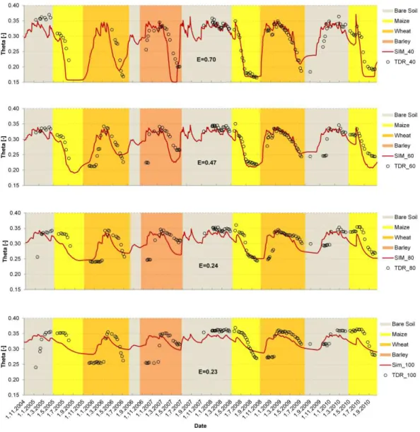
Volumetric water content was measured during the whole simulation period at 40 cm, 60 cm, 80 cm and 100 cm depths (Fig. 6). Good agreement between the measured and simulated TDR data was found at the 40 and 60 cm depths with model efficiency coefficients of 0.70 and 0.47, respectively. For the 80 and 100 cm depths, the volumetric water content was not as accurately described as for the upper layers, but still satisfactory model efficiency coefficients were achieved (E=0.24, E=0.23). The model performed better in terms of fitting volumetric water content during and after the calibration period (2008/2010) compared to the first years (2004/2007). For instance, the model efficiency coefficient for water content at 60 cm depth was E=0.64 for the period 2008/2010 and E=0.17 for the period 2004/2007. During the whole multiannual simulation, one single set of hydraulic properties was used. In order to have better fit to the measured values of volumetric water content, a real temporal dynamics of the topsoil hydraulic properties should be accounted for. Schwen et al. (2011) improved near-surface soil water simulations by accounting for time-variable hydraulic properties in a field undergoing different tillage practices. These authors found that the use of time-variable hydraulic parameters significantly improved simulation performance for all treatments, resulting in average relative errors below 13%. In complex 2D system resulting from large structural variability in the tilled layer, temporal effects could be expected to be even larger since the positions of the different structures in the tilled layer change after each ploughing (Roger-Estrade et al., 2000). Although they did not account for such time-dependent effects, the HYDRUS-2D simulations performed herein have
shown good reliability during a multiple years using just one set of soil hydraulic parameters calibrated on only one specific year.
3.2. Isoproturon transport
After water dynamics in the soil profile was satisfactorily modeled, isoproturon fate was simulated using the pesticide fate parameters from Table 1, assuming degradation only in liquid phase. The simulation showed a very large overestimation of the loss of isoproturon mass during the whole period (data not shown). The arrival time of isoproturon in the outflow was quite accurate, but the final mass leached was more than three orders of magnitude higher in the simulated outflow than in the measured one (1602 μg compared to 0.66 μg). This led to the assumption that the laboratory-measured degradation rates were too low to describe IPU dynamics in the field. Degradation rates for isoproturon (expressed as DT50 values) were taken from Vieublé-Gonod et al. (2009) and ranged from 10.3 to 19.2 days (for Γ, Δ, IF, and PP). For example, Walker et al. (2002) reported that the variation of IPU degradation rate in the field (expressed as DT50 values) ranged from 6 to 30 days. Cheviron and Coquet (2009) performed a sensitivity analysis on the fate of isoproturon in three types of soil and found that the tested model (HYDRUS- 1D) was highly sensitive to pesticide degradation rate. This suggests that the laboratory-measured pesticide fate parameters may not be always fully representative of the degradation processes affecting isoproturon in the field and hence some modifications of these parameters are needed to better describe IPU concentration at the outlet of the wick lysimeters. A second simulation was performed assuming degradation to take place in both the liquid and the solid phases (Guo et al., 2000). The degradation rate in solid phase was optimized having in mind that smaller microbiological activity should occur in the solid phase compared to the liquid phase. Satisfactory simulation results were achieved when using a degradation rate in solid phase set at 75% of that in liquid phase, with a model efficiency coefficient of 0.7 (Fig. 7). Optimization focused on degradation parameters since the arrival time of isoproturon in lysimeter outflow was already correctly simulated suggesting that IPU mobility was correctly parameterized. A sensitivity analysis of the IPU loss to degradation rate was performed. The optimized degradation rates (liquid and solid phase) were
increased or decreased by 50% for each structure/layer. The ratio of variation (ROV) was calculated in order to quantify the sensitivity of IPU loss to the degradation rate (liquid and solid phase) in each structure/layer. The ROV for solid phase degradation rate varied from -4.50 to -1.55 for the Γ structure; from -2.13 to -0.79 for Δ clods; from -1.99 to -0.80 for IF zones; from -0.58 to -0.36 for PP layer; and from -0.12 to -0.10 for E horizon. The ROV for liquid phase degradation rate had smaller variation with values from -0.31 to -0.26 for the Γ structure; from 0.11 to 0.10 for Δ clods; from -0.11 to -0.10 for IF zones; from -0.09 to -0.08 for PP layer; and from -0.04 to -0.04 for E horizon. The largest sensitivity was found in the Γ, Δ and IF, zones of the tilled layer, while PP and E horizons had very small values of | |. The sensitivity of the cumulative isoproturon mass loss was in order Γ Δ IF>PP>E, which revealed the fact that the spatial distribution of pesticide degradation rate plays a major role in its fate and dynamics (Walker et al., 2001).
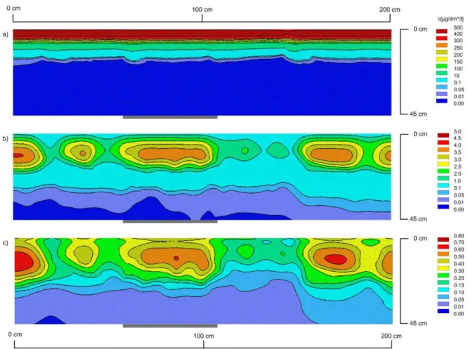
Different snapshots of the IPU concentration in the soil solution during 2007 are presented in Fig. 8. Isoproturon was applied on the 20th of February 2007 (Fig.1) at the rate of 1000 g per ha. After 13 days, the concentration of isoproturon was very high in the first 15 cm (Fig.8a) and the distribution was uniform along a longitudinal transect with a small exception at approximately x=140 cm where the concentration was lower. This was due to the presence of a compacted clod at the soil surface at this particular location (Fig. 2a). The low permeability of the compacted Δ clods redirected the flow toward Γ soil zones, as found by Coquet et al. (2005b), and toward IF soil zones. The effect is mostly seen after 137 and 186 days (Fig.8b, c) where low IPU concentrations are found at the location of the Δ clods. The lowest concentration was found at the approximately x= 110 – 140 cm at both times due to the placement of the Δ clod in the tilled layer at this location (Fig. 2a, b). Interfurrows had the largest flow velocity values in the tilled layer, with an average maximum velocity of 2.5 cm day-1in Γ zones to 8.7 cm day-1 in IF zone 137 days after application. However, due to the fast degradation rate in the IF (DT50 of 10.3 in liquid phase and 7.7 days in solid phase compared to 19.2 days in liquid phase and 14.4 in solid phase in the Γ soil zones), the highest IPU concentration was located in the Γ soil zones.
3.3. Sensitivity of water outflow and isoproturon loss to soil structure heterogeneity and to plough pan discontinuity in the tilled layer
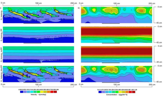
In addition to the long term simulations described above, three hypothetical scenarios were simulated: i) a homogeneous tilled layer with the presence of the plough pan as used for calibration; ii) a homogeneous tilled layer without plough pan iii) a heterogeneous tilled layer with a discontinuous plough pan. The discontinuity of the plough pan was located above the lysimeter plate and was approximately 50 cm large (from x= 109 to 159 cm). Γ structure was used instead of PP, to create this discontinuity. This last simulation was performed having in mind that during profile description some discontinuities of the plough pan were indeed observed locally albeit not quantified. The main goal of the simulations was to see how the presence of different structure arrangements influence water flow and pesticide transport. Simulations using a homogeneous tilled layer (Q_homog_PP, Fig.9) showed no major differences in water outflow pattern when compared to simulations accounting for tilled layer heterogeneity (Q_heterog). The cumulative amount of outflow was only 38 mm (3.6%) higher when a homogeneous tilled layer was considered. The absence of heterogeneity in the tilled layer caused a uniform water velocity field down to the plough pan (Fig.10a). Removing the plough pan in the homogeneous tilled layer scenario (Q_homog_noPP) caused smaller cumulative outflow (1065 mm compared to 1085 mm, i.e. 2%) than in the Q_homog_PP scenario. This effect could be related to the change in saturated hydraulic conductivity of the layer situated just below the tilled one (~28-38 cm), which was increased from 4.8 cm day-1 (PP) to 19.6 cm day-1 (). This change resulted in an increase in water flow velocity (Fig 10a) and caused more bypassing of the lysimeter plate. In the Q_heterog_discPP scenario, one can distinguish areas with high velocity just above and on the border of the plate where the discontinuity was placed. Inserting a discontinuous plough pan in the simulation domain increased the total cumulative outflow by 20% (from 1047 to 1252 mm, Fig.9). Increases in outflow occurred mostly during the high intensity rainfalls under wet soil conditions, which caused local saturation above the plough pan and lateral flow towards the surrounding more permeable soil
zones. A similar effect was observed by Coquet et al. (2005a) in a field experiment where the difference in saturated hydraulic conductivity between Γ and Δ soil zones forces flow streamlines around the Δ clods causing funneled flow. In the Q_heterog_discPP scenario, water flow paths of high velocities are connecting the high-conductivity interfurrows to the edges of the lysimeter plate thereby explaining the much higher cumulated outflow simulated for this scenario (Fig. 10a).
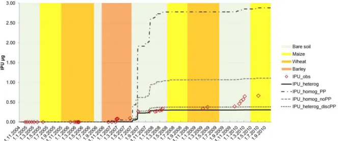
The different scenarios ended up with very different final IPU loss. All three scenarios showed an increase of IPU concentration in lysimeter outflow compared to base case scenario (IPU_heterog, Fig. 11). The largest increase was in the IPU_homog_PP scenario (+829%) which can be explained with the fact that the entire tilled layer had the same degradation rate as that of the Γ structure, which was lower than degradation rate of the and IF structures (Table 1). The other two scenarios IPU_homog_noPP and IPU_heterog_discPP had an increase of 258 and 22.6%, respectively compared to the base case scenario (IPU_heterog). In the case of the IPU_homog_noPP scenario, increased hydraulic conductivity below the tilled layer caused an increase in IPU transfer to deeper layers bypassing the wick lysimeters so that the increase in IPU loss was less than the one found for the IPU_homogPP scenario. Isoproturon distribution in the tilled layer differed according to the various scenarios (Fig. 10b). For the scenarios with a homogenous tilled layer (IPU_homogPP and IPU_homog_noPP), there was a uniform IPU distribution in the tilled layer with largest values located between 10 and 20 cm depth, although in the Q_homog_PP scenario it can be noticed that the IPU distribution at ~40 cm depth follows the upper border of the plough pan layer. Having a discontinuity in the plough pan caused larger isoproturon loss than in case when the plough pan was continuous (Fig. 11) due to higher velocities observed at the border of the plate (Fig.10b).
4. Conclusions
A long term (2004-2010) modeling study was performed on an agricultural field experiment to evaluate how the presence of heterogeneities due to soil tillage and compost application affect water flow and pesticide dynamics in soil. The study was done on a plot receiving a co-compost of green
wastes and sewage sludge (SGW) with winter wheat, barley and maize cultivation. Detailed profile description was used to locate different soil structures in the profile, which were then implemented in the HYDRUS-2D model. Volumetric water content (TDR), pressure head (tensiometers), water outflow and isoproturon concentration (wick lysimeters) were monitored in the field. Lysimeter outflow and water content dynamics in the soil profile were correctly described for the whole period (model efficiency coefficient: 0.99) after optimization of the soil hydraulic properties on one particular year and after some adaptation of LAI estimations for wheat (2005/06) and barley (2006/07). Using laboratory-measured degradation rates and assuming degradation to occur only in liquid phase caused large overestimation of simulated isoproturon losses in lysimeter outflow. After considering additional degradation in solid phase, whose rate was estimated to be 75% of the rate in liquid phase, a proper order of magnitude of isoproturon losses was simulated. Isoproturon concentrations were found to be highly sensitive to degradation rates. Different soil structures and zones in the tilled layer (Γ, IF, Δ ) had a large influence on the isoproturon distribution in the tilled layer, while the low permeability plough pan caused uniform water and solute distribution beneath it. Neither the laboratory-measured isoproturon fate parameters nor the independently-derived soil hydraulic parameters could describe the actual multiannual field dynamics of water and isoproturon without calibration. However, once calibrated on a limited period of time (9 months), HYDRUS-2D was able to simulate the whole 6-year time series with good accuracy.
Acknowledgements
This work was financially supported by GENESIS project on groundwater systems financed by the European Commission FP7 large-scale project contract 226536. We acknowledge the Veolia Environment group for financial support of the QUALIAGRO field site. We thank Christophe Labat for the installation of the wick lysimeters, the field measurements of soil hydraulic conductivity and the characterization of other soil physical properties (bulk densities and water retention properties at
the profile scale). Guillaume Bodineau, Vincent Mercier and Jean-Noel Rampon are greatly acknowledged for their support in the field instrumentation and monitoring.
References
1. Ankeny MD, Kaspar TC, Horton R. Characterization of tillage and traffic effects on unconfined infiltration measurements. Soil Sci Soc Am J 1990;54:837–40.
2. Brisson N, Ruget F, Gate P, Lorgeou J, Nicoullaud B, Tayot X, Plenet D, Jeuffroy MH, Bouthier A, Ripoche D, Mary B, Justes E. STICS: a generic model for simulating crops and their water and nitrogen balances. II. Model validation for wheat and maize. Agronomie 2002:22;69–92.
3. Chalhoub M, Coquet Y, Vachier P. Water and bromide dynamics in a soil amended with different urban composts. Vadose Zone J 2013;12:1-11.
4. Cheviron B, Coquet, Y. Sensitivity analysis of transient-MIM HYDRUS-1D: case study related to pesticide fate in soils. Vadose Zone J 2009:8;1064–79.
5. Coquet Y, Coutadeur C, Labat C, Vachier P, van Genuchten MTh, Roger-Estrade J, Šimůnek J. Water and solute transport in a cultivated silt loam soil: I. Field observations. Vadose Zone J 2005a;4:573–86.
6. Coquet Y, Šimůnek J, Coutadeur C, van Genuchten MTh, Pot V, Roger-Estrade J. Water and solute transport in a cultivated silt loam soil: 2. Numerical analysis. Vadose Zone J. 2005b;4:587–601. doi:10.2136/vzj2004.0153
7. Coutadeur C, Coquet Y, Roger-Estrade J. Variation of hydraulic conductivity in a tilled soil. Eur J Soil Sci 2002;53:619–28.
8. De wilde T, Mertens J, Spanoghe P, Ryckeboer J, Jaeken P, Springael D. Sorption kinetics and its effects on retention and leaching. Chemosphere 2008;72:509–16.
9. Dousset S, Thevenot M, Pot V, Šimůnek J, Andreux F. Evaluating equilibrium and non-equilibrium transport of bromide and isoproturon in disturbed and undisturbed soil columns. J Contam Hydrol 2007;94:261–76.
10. Dubus IG, Brown CD, Beulke S. Sensitivity analyses for four pesticide leaching models. Pest Manag Sci 2003;59:962–82. doi:10.1002/ps.723
11. Feddes RA, Kowalik PJ, Zaradny H Simulation of Field Water Use and Crop Yield. John Wiley & Sons, New York; 1978.
12. Guo L, Bicki TJ, Felsot AS, Hinesly TD. Sorption and movement of alachlor in soil modified by carbon-rich wastes. J Environ Qual 1993;22:186–94.
13. Guo L, Jury WA, Wagenet RJ, Flury M. Dependence of pesticide degradation on sorption: nonequilibrium model and application to soil reactors. J Contam Hydrol 2000;43:45–62. 14. Gupta SC, Dowdy RH, Larson WE. Hydraulic and thermal properties of a sandy soil as
influenced by incorporation of sewage sludge. Soil Sci Soc Am J 1977;41:601–605.
15. Gӓrdenӓs AI, Šimůnek J, Jarvis N, van Genuchten MTh. Two-dimensional modelling of preferential water flow and pesticide transport from a tile-drained field. J Hydrol 2006;329:647–60.
16. Hopmans JW, Šimůnek J., Romano N., Durner W. Simultaneous determination of water transmission and retention properties. Inverse methods. p. 963–1008. In Dane JH. Topp GC. (ed.) Methods of soil analysis. Part 4. Physical methods. SSSA Book Ser. 5. SSSA, Madison, WI; 2002.
17. Houot S, Cambier Ph, Benoit P, Deschamps M, Jaulin A, Lhoutellier C. Effect of repeated compost applications on availability of organic and metallic micropollutants in soil [in French]. Etude et Gestion des Sols 2009;16:255–74.
18. Jarvis NJ. A review of non-equilibrium water flow and solute transport in soil macropores: principles, controlling factors and consequences for water quality. Eur J Soil Sci 2007;58:523– 46.
19. Javaux M, Kasteel R, Vanderborght J, Vanclooster M. Interpretation of dye transport in a macroscopically heterogeneous unsaturated subsoil with a 1-D model. Vadose Zone Journal 2006;5:529–38.
20. Jury WA, Spencer WF, Farmer WJ. Behavior assessment model for trace organics in soil: I. Model description. J Environ Qual 1983;12:558– 64.
21. Kay B. Rates of change of soil structure under different cropping systems. Adv Soil Sci 1990;12:1–52.
22. Klute A, Dirksen C. Hydraulic conductivity and diffusivity: laboratory methods. In: Methods of Soil Analysis. Part 1. Physical and Mineralogical Methods. Agronomy Monograph no. 9. ASA-SSSA: Madison, USA, 1986.
23. Knutson JH, Selker JS. Unsaturated hydraulic conductivities of fiberglass wicks and designing capillary wick pore-water samplers. Soil Sci Soc Amer J 1994;58:721–9.
24. Kodešová R, Kočárek M, Kodeš V, Drábeka O, Kozák J, Hejtmánkovác K. Pesticide adsorption in relation to soil properties and soil type distribution in regional scale. J Hazard Mater 2011;186:540–50.
25. Kodešová R, Kozák J, Šimůnek J, Vacek O. Single and dual permeability model of chlorotoluron transport in the soil profile. Plant Soil Environ 2005;51:310–15.
26. Köhne JM, Köhne S, Šimůnek J. Multi-process herbicide transport in structured soil columns: experiments and model analysis. J Contam Hydrol 2006;85:1–32.
27. Manichon H, Roger-Estrade J. Characterization of soil structure and its evolution at short and medium term due to cropping system effects. [in French] In Picard D, Combe L. (ed.) Les systémes de culture. INRA Editions, Paris. 1990:27–55.
28. Manichon H. Influence of cropping systems on the cultivation profile: development of a diagnostic method based on morphological observation [in French]. PhD thesis, INRA, Paris; 1982.
30. Mualem Y. A new model for predicting the hydraulic conductivity of unsaturated porous media. Water Resour Res 1976;12:513–22.
31. Mubarak I, Mailhol JC, Angulo-Jaramillo R, Ruelle P, Boivin P, Khaledian M. Temporal variability in soil hydraulic properties under drip irrigation. Geoderma 2009;150:158–65. 32. Nash JE, Sutcliffe JV. River flow forecasting through conceptual models. Part I. A discussion
of principles J Hydrol 1970;10:282–90.
33. Or D, Leij FJ, Snyder V, Ghezzehei TA. Stochastic model for posttillage soil pore space evolution. Water Resour Res 2000;36(7):1641–52.
34. Pot V, Benoit P, Etievant V, Bernet N, Labat C, Coquet Y, Houot S. Effects of tillage practice and repeated urban compost application on bromide and isoproturon transport in a loamy Albeluvisol. Eur J Soil Sci 2011;62:797–810.
35. Pot V, Šimůnek J, Benoit P, Coquet Y, Yra, A., Martinez-Cordon MJ. Impact of rainfall intensity on the transport of two herbicides in undisturbed grassed filter strip soil cores. J Contam Hydrol 2005;81(1–4):63–88.
36. Reynolds WD, Elrick DE. Determination of hydraulic conductivity using a tension infiltrometer. Soil Sci Soc Am J 1991;55:633–9.
37. Roger-Estrade J, Richard G, Boizard H, Boiffin J, Caneill J, Manichon H. Modelling structural changes in tilled topsoil over time as a function of cropping systems. Eur J Soil Sci 2000; 51:455–474.
38. Schneider S, Coquet Y, Vachier P, Labat C, Roger-Estrade J, Benoit P, Pot V. Houot S. Effect of urban waste compost application on soil near-saturated hydraulic conductivity. J Environ Qual 2009;38:772–81.
39. Schwen A, Bodner G, Loiskandl W. Time-variable soil hydraulic properties in near-surface soil water simulations for different tillage methods. Agric Water Manage 2011;99:42-50. 40. Simon N. Reactivity of dissolved organic matter and pesticide mobility under different land
41. Šimůnek J, van Genuchten MTh, Šejna M. Development and Applications of the HYDRUS and STANMOD Software Packages and Related Codes. Vadose Zone J. 2008;7:587–600. doi:10.2136/vzj2007.0077
42. SOeS French national service for the environment. Groundwater contamination by pesticides [in French]. 2012.
43. Strudley MW, Green TR, Ascough JC. Tillage effects on soil hydraulic properties in space and time: State of the science. Soil Tillage Res. 2008;99:4–48.
44. Stumm W, Morgan JJ. Aquatic Chemistry: An Introduction Emphasizing Chemical Equilibria in Natural Waters. John Wiley & Sons, New York; 1981.
45. van Genuchten MTh, Leij FJ, Yates SR. The RETC Code for Quantifying the Hydraulic Functions of Unsaturated Soils, Version 1.0. EPA Report 600/2-91/065, U.S. Salinity Laboratory, USDA, ARS, Riverside, California; 1991.
46. van Genuchten, M.Th. A closed-form equation for predicting the hydraulic conductivity of unsaturated soils. Soil Sci Soc Am J 1980;44:892–8.
47. Vanclooster M, Javaux M, Vanderborght J. Solute transport in soil at the core and field scale. In: Anderson MG, McDonnell JJ. (Eds.) Encyclopedia of Hydrological Sciences. Wiley; 2005. 48. Vieublé-Gonod L, Benoit P, Cohen N, Houot S. Spatial and temporal heterogeneity of soil microorganisms and isoproturon degrading activity in a tilled soil amended with urban waste composts. Soil Biol Biochem 2009;41:2558–67.
49. Vogel T, van Genuchten MTh. Cislerova M. Effect of the shape of the soil hydraulic functions near saturation on variably-saturated flow predictions. Adv Water Resour 2001;24:133–44. 50. Walker A, Bromilow RH, Nicholls PH, Evans AA, Smith VJR. Spatial variability in the
degradation rates of isoproturon and chlorotoluron in a clay soil. Weed Res 2002;42:39–44. 51. Walker A, Jurado-Exposito M, Bending GD, Smith VJR. Spatial variability in the degradation
rate of isoproturon in soil. Environ Pollut 2001;111:407–415.
52. Walker A. A simulation model for prediction of herbicide persistence. J Environ Qual 1974;3:396–401.
53. Wesseling JG. Multi-year simulations of groundwater resources for different soil types, aquifer settings and crops with the model SWATRE [in Dutch]. SC-DLO report 152, Wageningen, the Netherlands; 1991.
54. Xu D, Mermoud A. Modeling the soil water balance based on time-dependent hydraulic conductivity under different tillage practices. Agric Water Manage 2003;63:139–51.
Tables:
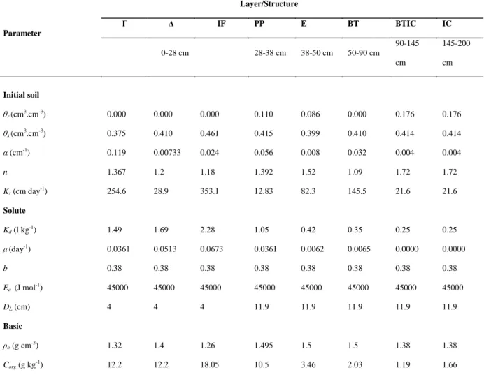
Table 1. Physical and chemical input parameters required by the HYDRUS 2D model.
Parameter Layer/Structure Γ Δ IF PP E BT BTIC IC 0-28 cm 28-38 cm 38-50 cm 50-90 cm 90-145 cm 145-200 cm Initial soil θr (cm3.cm-3) 0.000 0.000 0.000 0.110 0.086 0.000 0.176 0.176 θs (cm3.cm-3) 0.375 0.410 0.461 0.415 0.399 0.410 0.414 0.414 α (cm-1) 0.119 0.00733 0.024 0.056 0.008 0.032 0.004 0.004 n 1.367 1.2 1.18 1.392 1.52 1.09 1.72 1.72 Ks (cm day-1) 254.6 28.9 353.1 12.83 82.3 145.5 21.6 21.6 Solute Kd (l kg-1) 1.49 1.69 2.28 1.05 0.42 0.35 0.25 0.25 μ(day-1) 0.0361 0.0513 0.0673 0.0361 0.0062 0.0065 0.0000 0.0000 b 0.38 0.38 0.38 0.38 0.38 0.38 0.38 0.38 Ea(J mol-1) 45000 45000 45000 45000 45000 45000 45000 45000 DL (cm) 4 4 4 11.9 11.9 11.9 11.9 11.9 Basic ρb (g cm-3) 1.32 1.4 1.26 1.495 1.5 1.5 1.38 1.38 Corg (g kg-1) 12.2 12.2 18.05 10.5 3.46 2.03 1.19 1.66
θr – residual water content, θs– saturated water content, α and n – van Genuchten-Mualem shape parameters, Ks– saturated hydraulic
conductivity, Kd– sorption coefficient, μ – isoproturon degradation rate, b – Walker’s exponent, Ea– energy of activation for the degradation
rate, DL– longitudinal dispersivity, ρb– bulk density, Corg– organic carbon content.
Table 2. van Genuchten soil hydraulic parameters after calibration.
Parameter
Layer/Structure
Γ Δ IF PP E BTI BTII BTICI BTICII IC
0-28 cm 28-38 cm 38-50 cm 50-70 cm 70-90 cm 90-120 cm 120-145 cm 145-200 cm θr (cm3.cm-3) 0.0002 0.000 0.000 0.105 0.000 0.0006 0.0006 0.000 0.000 0.000 θs (cm3.cm-3) 0.410 0.410 0.461 0.455 0.38 0.37 0.38 0.37 0.36 0.3 α (cm-1) 0.0385 0.00733 0.024 0.042 0.015 0.024 0.028 0.02 0.029 0.032 n 1.14 1.2 1.18 1.1 1.17 1.12 1.12 1.09 1.12 1.1 Ks (cm day-1) 19.6 2.8 353.1 4.8 14 5.8 7.9 3.8 3.7 8
List of Figures
Fig. 1. Crop calendar with the different agricultural operations (e.g. sowing, tillage, harvest) including isoproturon applications.
Fig. 2. (a) Field soil profile description including the different soil structures observed in the tilled layer and (b) spatial distribution of the different soil structures and soil layers used in the HYDRUS-2D model together with the location of the wick lysimeters. Horizons BT and BT/IC were split into two layers for the sake of model optimization.
Fig. 3. Observed (symbols) vs simulated (line) values of cumulative lysimeter outflow (left) and precipitation distribution (right) during the calibration period.
Fig. 4. Observed (symbols) vs simulated (line) values of volumetric water content (left) and pressure head (right) at different depths (20, 40, 60, 80, 100, 130, 160 cm depth).
Fig. 5. Observed (symbols) vs simulated (line) cumulative lysimeter outflow using calibrated soil hydraulic parameters before (Q_sim) and after (Q_sim_opt) LAI optimization.
Fig. 6. Observed symbols) vs simulated (line) volumetric water content using calibrated soil hydraulic parameters after LAI optimization from 2004 till 2010 at 40, 60, 80, and 100 cm depth.
Fig. 7. Observed (symbols) vs simulated (line) values of isoproturon loss in lysimeter outflow from 2004 till 2010 assuming degradation in solid phase.
Fig. 8. Isoproturon concentration distribution in the soil solution in the topsoil at different times: a) 13, b) 137, and c) 186 days after the second application (dated 20 February 2007).
Fig. 9. Observed (symbols) vs simulated (lines) cumulative lysimeter outflow using calibrated soil hydraulic parameters with different soil structure distributions in the topsoil (Q_heterog – heterogeneous tilled layer with plough pan; Q_homog_PP – only Γ structure in the tilled layer with plough pan; Q_homog_noPP – Γ structure without plough pan; Q_heterog_discPP –heterogeneous tilled layer with a discontinuous plough pan).
Fig. 10. Water velocity (a) and IPU distribution (b) in the topsoil for various scenarios 186 days after the second IPU application (25 August 2007): Q_heterog –heterogeneous tilled layer with plough pan; Q_homog_PP – only Γ structure in the tilled layer with plough pan; Q_homog_noPP – Γ structure without plough pan; Q_heterog_discPP –heterogeneous tilled layer with a discontinuous plough pan.
Fig. 11. Observed (symbols) vs simulated (lines) isoproturon loss in lysimeter outflow using calibrated soil hydraulic parameters with different soil structure distributions in the topsoil (IPU_heterog – heterogeneous tilled layer with plough pan; IPU_homog_PP – only Γ structure in the tilled layer with plough pan; IPU_homog_noPP – Γ structure without plough pan; IPU_heterog_discPP – heterogeneous tilled layer with a discontinuous plough pan) during 2004 - 2010.