A diagnostic analysis of retail out-of-stocks

A Diagnostic Analysis of Retail Out-of-Stocks

by

Yong Ning Foo

B.Eng., Electrical Engineering, National University of Singapore (2006)

Submitted to the School of Engineering

in Partial Fulfillment of the Requirements for the Degree of

Master of Science in Computation for Design and Optimization

at the

MASSACHUSETTS INSTITUTE OF TECHNOLOGY

September 2007

© Massachusetts Institute of Technology 2007. All rights reserved.

A

Author...

...

School of Engineering

August 16 2007

Certified by...

...

.

...

Stephen C. Graves

Abraham J. Siegel Professor of Management Science

Thesis Supervisor

L

j

A/i

Jaime

Peraire

Accepted by...

Professor of Aeronautics and Astronautics

Codirector, Computation for Design and Optimization Program

BARKER

CF TECHNOLOGY

SEP

7

7 2007

A Diagnostic Analysis of Retail Out-of-Stocks

by

Yong Ning Foo

Submitted to the School of Engineering on August 16, 2007, in partial fulfillment of the

requirements for the degree of

Master of Science in Computation for Design and Optimization

Abstract

In the highly competitive retail industry, merchandize out-of-stock (OOS) is a significant and pertinent problem. This thesis performs a diagnostic analysis on retail out-of-stocks using empirical data from a major retailer.

In this thesis, we establish the empirical relationship of OOS rate with the amount of safety stock carried, the time between orders and the forecast error, providing insights to the effects of these three factors on the probability of OOS occurrences.

The root causes of OOS are also examined in the thesis. We find that up to 34% of OOS

can be attributed to forecast error while up to 22% can be attributed to delay in order replenishment. For the OOSs that were associated with order delay, we can trace 60% of these to out-of-stock at the store's distribution center (DC).

The thesis also examines a peculiarity in the occurrence of OOSs. We found that the OOS rate of Class C items is significantly higher in stores with higher sales volume. We can attribute much of this phenomenon to three factors: stores with higher sales volume hold less safety stock for Class C items, have a shorter time between orders and have relatively larger forecast errors.

Thesis Supervisor: Stephen C. Graves

Acknowledgement

I am deeply grateful to Professor Stephen C. Graves for the great opportunity to work with

him. His clarity in thoughts, analytical insights and attention to details is inspirational. I will also never forget his willingness to address my academic and personal concerns during the course of the project.

I am thankful to the collaborators from Beta for making this project possible. I would love to name these wonderful individuals but I guess that would render the idea of anonymous reference pointless.

My gratitude extends to Xin, who took the time to attend all the meetings and provide

valuable suggestions and comments.

I would also like to show my appreciation to the Singapore-MIT Alliance for awarding me

the Graduate Fellowship. The experience, like many others, has been invaluable.

I must thank my Mom, Dad and my brother, Don for everything that they have given me

all these years. To Candice, who takes such an important place in my heart, I thank her for the unconditional love and support she has shown for the last 5 years.

I would also like to thank my friends Zhengyi, Fabian, Joline, Rebecca, Xu Song, Jia Chuan, Heidi and Fang Fang for making my stay in MIT much more fun and enjoyable; my roommate, Vinay, who has graciously allowed his table to be a part of my extended workspace; Jocelyn and John from SMA office for the awesome trips and dinners; and

Contents

List of Figures...10

List of Tables...12

Chapter 1 Introduction ... ₁₅

1.1 Company Background... ₁₅

1.2 Company's Inventory Policies... 15

1.2.1 The Order-Up-To-Level (R, S) Control System ... 16

1.2.2 Replenishment Frequency and Constraints... 17

1.2.3 Classification of SKUs... ₁₇

1.3 Project Motivation and Description... 18

1.4 Literature Review ... 19

1.4.1 Factors influencing Out-of-Stock Rates ... 19

1.4.2 Root Causes of Out-of-Stocks ... 20

1.5 Thesis Overview... ₂₀

Chapter 2 Data Description and Definitions ... 21

2.1 Description of Data Set

...

21

2.1.1 Inventory Data .. e ... 22

2.1.2 Store D ata ... 24

2.1.3 M erchandize Data... ₂₄

2.2 Preprocessing of Data ... 25

2.2.1 Removing Excess Data... .... 25

2.2.2 Removing Inaccurate Data... 25

2.2.3 Dealing wZ... ih ccrateD at ... 25

2..3 Dei inw _{th. Zer.F. reca... 26}

2.3 D efin itio n s

...

_{2 6}

Chapter 3 Empirical Model of OOS Rate ... 29

3.1 Out-of-Stock Rate and Safety Stock ... 29

3.2 Out-of-Stock Rate and Time Between Orders... 33

3.3 Out-of-Stock Rate and Normalized Forecast Error... 36

Chapter 4 Out-of-Stock Causes and Conditions ... 39

4.1 General OOS Causes in Retail Stores... 39

4.2 Algorithm to Determine OOS Causes... 40

4.2.1 Description of Algorithm... 40

4.2.2 Discussion on Algorithm Accuracy... 44

4 .3 R esults... ... 45

Chapter 5 Examining a Peculiarity ... 51

5.1 T h e P eculiarity ...---... 51

5.2 Peculiarity is not by Chance ... 53

5.2 .1 A N O V A ... 53

5.2.2 Multiple Hypothesis Tests ... 55

5.3 Three Causes of the Peculiarity Identified ... 56

5.3.1 Differences in Weeks of Safety Stock Carried... 56

5.3.2 Differences in Time Between Orders ... 59

5.3.3 Differences in Normalized Forecast Error ... 62

5.4 Other Hypothesized Causes that are not True... 64

Chapter 6 Conclusion ... .. 67

Appendix A Data for Exchange Curve of OOS Rate and WEEKS.SS ... 69

Appendix B Data for Exchange Curve of OOS Rate and TBO ... 73

Appendix C Data for Exchange Curve of OOS Rate and NFE ... 77

Appendix D Data on OOS Causes ... 83

Appendix E Data on OOS Rate of CLASS C SKUs By Stores...85

Appendix F Data on Relative Frequency of WEEKS.SS of CLASS C SKUs in RANK A Stores ... ... 87

Appendix G Data on Relative Frequency of TBO of CLASS C SKUs in RANK A Stores... ... 89

Appendix H Data on Relative Frequency of NFE of CLASS C SKUs in RANK A

Stores... ₉₁

Appendix I Distribution of Stores by OOS Rate of CLASS C SKUs ... 95

Appendix

J

SKUs that have Higher OOS Rate...97 R eferences: ... ₁₀₁

List of Figures

Figure 3.1: Plot of OOS rate against WEEKS.SS for CLASS A items ... 31

Figure 3.2: Plot of OOS rate against WEEKS.SS for CLASS B items... 31

Figure 3.3: Plot of OOS rate against WEEKS.SS for CLASS C items...32

Figure 3.4: Plot of OOS rate against WEEKS.SS for New items ... 32

Figure 3.5: Plot of OOS rate against TBO for CLASS A items ... 34

Figure 3.6: Plot of OOS rate against TBO for CLASS B items ... 34

Figure 3.7: Plot of OOS rate against TBO for CLASS C items ... 35

Figure 3.8: Plot of OOS rate against TBO for New items ... 35

Figure 3.9: Plot of OOS rate against NFE for CLASS A items ... 37

Figure 3.10: Plot of OOS rate against NFE for CLASS B items ... 37

Figure 3.11: Plot of OOS rate against NFE for CLASS C items...38

Figure 3.12: Plot of OOS rate against NFE for New items...38

Figure 4.1: Summary of distribution of OOS causes at retail stores in general [6] ..40

Figure 4.2: Plot of percentage occurrence of OOS causes and conditions...46

Figure 4.3: Plot of percentage occurrence of OOS causes and conditions, split by SKU CLA SS ... 46

Figure 4.4: Plot of percentage occurrence of major OOS. ... 47

Figure 4.5: Plot of percentage occurrence of major OOS causes normalized to 100% for each forecast error type...-47

Figure 4.6: Key OOS Causes...-49

Figure 5.1: OOS rate aggregated by SKU CLASS and STORE RANK...52

Figure 5.2: OOS rate of CLASS C SKUs aggregated by SKU.DIV and RANK...52

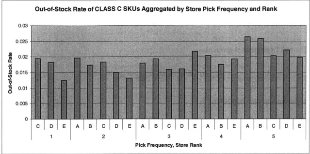
Figure 5.3: OOS Rate of CLASS C SKUs aggregated by PF and RANK...53

Figure 5.4: Box Plot of the OOS Rate of the Stores... ... 54

Figure 5.5: Relative frequency of safety stock in weeks in RANK A Stores ... 57

Figure 5.6: Relative frequency of safety stock in weeks in RANK E Stores ... 57

Figure 5.7: Relative frequency of time between orders in RANK A Stores ... 60

Figure 5.8: Relative frequency of time between orders in RANK E Stores ... 61

Figure 5.9: Relative frequency of normalized forecast error in RANK A Stores...63

Figure 5.10: Relative frequency of normalized forecast error in RANK E Stores...63

Figure 1.1: Distribution of RANK A stores by OOS of CLASS C SKUs...95

Figure 1.2: Distribution of RANK B stores by OOS of CLASS C SKUs ... 95

Figure 1.3: Distribution of RANK C stores by OOS of CLASS C SKUs ... 96

Figure 1.4: Distribution of RANK D stores by OOS of CLASS C SKUs...96

Figure 1.5: Distribution of RANK E stores by OOS of CLASS C SKUs ... 96

Figure J.1: OOS Rate of CLASS C items grouped by difference in relative frequency in RANK A and RANK E stores ... 98

List of Tables

Table 4.1: Distribution of OOS Causes ... 48

Table 5.1: P values of the hypothesis tests ... 55

Table 5.2: Degrees of freedom of the hypothesis tests...56

Table 5.3: WEEKS.SS Model and Actual OOS Rate...59

Table 5.4: Percentage Responsibility of WEEKS.SS...59

Table 5.5: TBO Model and Actual OOS Rate... 61

Table 5.6: Percentage Responsibility of TBO...62

Table 5.7: NFE Model and Actual OOS Rate...64

Table 5.8: Percentage Responsibility of NFE...64

Table A.1: Data for OOS Rate versus WEEKS.SS, all SKUs...69

Table A.2: Data for Table A.3: Data for Table A.4: Data for Table A.5: Data for Table B.1: Data for Table B.2: Data for Table B.3: Data for Table B.4: Data for Table B.5: Data for Table C.1: Data for Table C.2: Data for Table C.3: Data for Table C.4: Data for OOS Rate versus WEEKS.SS, CLASS A SKUs only...70

OOS Rate versus WEEKS.SS, CLASS B SKUs only ... 70

OOS Rate versus WEEKS.SS, CLASS C SKUs only ... 71

OOS Rate versus WEEKS.SS, New SKUs only...72

OOS Rate versus TBO, all SKUs...73

OOS Rate versus TBO, CLASS A SKUs only...74

OOS Rate versus TBO, CLASS B SKUs only ... 74

OOS Rate versus TBO, CLASS C SKUs only ... 75

OOS Rate versus TBO, New SKUs only...76

OOS Rate versus NFE, All SKUs ... 77

OOS Rate versus NFE, CLASS A SKUs ... 78

OOS Rate versus NFE, CLASS B SKUs only ... 79

OOS Rate versus NFE, CLASS C SKUs only ... 80

Table C.5: Data for OOS Rate versus NFE, New SKUs only... 81

Table D.1: Data on frequency of occurrence of OOS conditions ... 83

Table D.2: Data on frequency of occurrence of OOS conditions, split by CLASS... 83

Table E.1: Data on the OOS rate of CLASS C SKUs by stores ... 85

Table F.1: Data on relative frequency of SS of CLASS C SKUs in A Stores...87

Table F.2: Data on relative frequency of SS of CLASS C SKUs in E Stores ... 88

Table G.1: Data on relative frequency of TBO of CLASS C SKUs in A Stores ... 89

Table G.2: Data on relative frequency of TBO of CLASS C SKUs in E Stores ... 90

Table H.1: Data on relative frequency of NFE of CLASS C SKUs in A Stores ... 91

Table H.2: Data on relative frequency of NFE of CLASS C SKUs in E Stores...92

Table J.1: Data on OOS Rate of CLASS C items grouped by difference in relative frequency in RANK A and RANK E stores ... 98

Chapter 1

Introduction

In the highly competitive retail industry, merchandize out-of-stock has been recognized as a significant problem. Using real data from a major retailer, we examine in this thesis the interdependencies of out-of-stock rate with various factors and we identify the root causes for out-of-stocks. We also look in depth into a peculiarity in the out-of-stock rate of the company, which serves to provide insights into the factors affecting the out-of-stock rate.

1.1 Company Background

The company is a United States based major retailer with over 1,000 retail stores and

10,000 SKUs. Due to confidentiality, we will refer to the company by the disguised name

of Beta.

1.2 Company's Inventory Policies

Beta carries approximately 6,300 SKUs per store, which are replenished either from the

DC or directly from the supplier (or distributor) by a flow through policy. About 70% of

the SKUs are replenished from the DC while the remaining items are replenished by the flow through policy.

Each store is replenished on a regular replenishment cycle based on its pick frequency, which specifies the number of times the store is replenished per week. For example, a pick frequency of 2 would mean that the store is replenished twice a week.

Beta manages the inventory in its retail stores primarily with a periodic-review, order-up-to-level (R, S) control system [9] with replenishment constraints. The review period is one day with review at the end of each day.

1.2.1 The Order-Up-To-Level (R, S) Control System

For each item (or SKU) and each retail store, the inventory control system generates a seasonalized weekly forecast using past sales performance. For each item and each retail store, the inventory control system computes the amount of safety stock required, based on the forecast, the service level, the replenishment lead time and the pick frequency for the store. We term this safety stock as "system generated safety stock" and denote it as

SYS.SS. The system allows managers to set for each item and store, the minimum

presentation stock, MIN.P; this is the minimum number of units the manager wishes the item to have on the shelf at all time.

As shown by equation 1.1, the greater of the safety stock and minimum presentation, gives the amount of safety stock that the system uses to calculate the re-order point and the order up to level.

SS

=

max(SYS.SS

,

MIN.P).

(1.1)

Thus, the minimum presentation can be viewed as a restricted form of override for the system generated safety stock; the minimum presentation can be used to increase the amount carried but never to decrease it. In order to compute the re-order point, we first need to compute the vendor order point (VOP), which is given as,

VOP

=

max(SYS.SS

,

MIN.P) + LT.UNITS + VCS,

(1.2)

where SYS.SS, MIN.P, LT.UNITS and VCS are the safety stock, minimum presentation,

ROP

max(VOP, BUYR.MIN )-1.

Items are re-ordered when their inventory position (inventory on hand plus inventory on order) is equal to or lower than the reorder point.

The system computes an order-up-to-level, which we denote as SYS.OUTL, by adding the item cycle stock to the reorder point given by equation (1.3). Managerial control over the order-up-to-level is provided by two adjustable parameters: the buyer maximum and the hard maximum denoted by BUYR.MAX and HARD.MAX respectively. These parameters allow the manager to decrease the order-up-to-level. The BUYR.MAX is a soft stop in the sense that the system would ignore it if the service level goal cannot be achieved. The

HARD.MAX however is a hard stop. We use OUTL to denote the final order-up-to-level

after considering BUYR.MAX and HARD.MAX.

1.2.2 Replenishment Frequency and Constraints

The pick frequency of a store depends on its sales volume. It goes as high as 5 times per week for high volume stores and as low as once per week for low volume stores. Stores do not replenish on Sunday.

1.2.3 Classification of SKUs

Beta categorizes their SKUs into five divisions based on their intrinsic properties. In this study, we examine SKUs from all five divisions.

Within each division, the SKUs are classified into priority ratings of CLASS A, CLASS B

and CLASS C that correspond to the 2 0th 3 0th and 5 0th percentile of the SKUs' sales

classified as CLASS A, the next 30% as CLASS B and the final 50% as CLASS C. This classification is done at the store level, which means that the same SKU may have a different priority rating at different stores. SKUs that are new and thus have no prior sales information are simply classified as New.

Beta uses a different service level target (percent in stock) for each product class, with

CLASS A having the highest target and CLASS C having the lowest.

1.3 Project Motivation and Description

In the highly competitive retail industry, merchandize in-stock has been recognized as an important factor in sales growth. A higher level of merchandize in-stock is associated with increased sales and greater customer satisfaction, and thus is an important competitive advantage. The problem of OOS is compounded by the ever increasing number of SKUs carried by retailers. It has been found that a larger assortment may lead to an increased risk of OOS occurrence [2][3], making it much more challenging to keep products in stock and available at all time.

In the recent years, two key developments had led to the urgency and significance of the

OOS issues. The first development is the increasing consumers' intolerance of OOS

situations [6]. With more purchasing channels, alternative outlets and information, consumers are increasingly likely to make their purchases elsewhere when encountered with an OOS.

The second development is the advent of technologies that allow retailers new ways to manage OOS issues [6] without incurring the huge costs in increased labor or greater inventory safety stock associated with traditional recommendations.

This thesis will examine the root causes of out-of-stocks and establish the inter-dependencies between out-of-stock rate and various factors.

1.4 Literature Review

While the significance of out-of-stock (OOS) issues in retail has been pointed out as early as the 60s by practitioners and researchers [7], recent advances in Category Management and Electronic Data Interchange have led to a renewed interest in the causes, extent and impact of out-of-stocks [3] [4].

A rather extensive research on the extent and causes of retail out-of-stocks is reported in [6]. The report examines the extent and magnitude of out-of-stocks in the fast moving

consumer goods (FMCG) industry worldwide and identifies the root causes of out-of-stocks. Other empirical studies on the factors affecting out-of-stocks can be found in

[1][3][5]. Due to the large number of factors that can impact out-of-stocks, we will review

only factors that are of most relevance.

1.4.1 Factors influencing Out-of-Stock Rates

The intuitive reasoning that higher inventory levels correspond to lower out-of-stock rates is rejected by [6]. It shows, using data from a few studies that there is a positive correlation between out-of-stock rates and the amount of safety stock carried. It argues that excessive backroom inventory may impede shelf replenishment and may indicate the presence of ineffective in-store inventory management and ordering systems.

It is suggested in [6] that out-of-stock rates are higher on promoted items. The conclusion is based on the fact that among the studies examined, all those that report promotional effects find substantially greater out-of-stock rates on promoted items than everyday items.

We would like to note here the possibility of self-selection bias in the reports - studies that

did not find a relationship between out-of-stock rates and promotion are less likely to report it.

[1] [3] [5] suggest that larger SKU assortments may lead to an increased risk of out-of-stock

which impacts faster moving items more severely due to constraints on minimum ship pack.

1.4.2 Root Causes of Out-of-Stocks

[6] attributes up to 50% responsibility for out-of-stocks to retail store ordering and

forecasting, 25% to execution issues and 25% to upstream causes. The findings suggest that most of the direct causes of out-of-stocks lie at the retail store level.

1.5 Thesis Overview

In Chapter 2 we present a detailed description of the dataset used in our analysis, describe the pre-processing procedures and state several definitions that will be used throughout the thesis. In Chapter 3 we establish the empirical relationship of out-of-stock (OOS) rate with safety stock and forecast error while in Chapter 4 we examine the root causes of OOS. In Chapter 5 we look in detail at a peculiarity whereby the out-of-stock rate of CLASS C items is higher in RANK A (highest volume) stores than in RANK E (lowest volume) stores. Chapter 6 concludes the thesis and provides some suggestions on further work.

Chapter 2

Data Description and Definitions

In this chapter, we provide a detailed description on the data set used in our analysis, describe the pre-processing procedures and state several definitions that we use throughout the thesis. We do not describe fields that were captured by the database but were not used in our analysis.

2.1 Description of Data Set

The data was collected from 233 stores located in the Northeastern region of United States over a period of 11 weeks. All stores are replenished from a common DC (distribution center) and carry a similar range of merchandize. Only active SKUs are included in the data set. By active SKUs we include all SKUs that were physically available on the store shelves at any time during the 11-week period.

There are three types of data that were collected: inventory data, store data and merchandize data. Inventory data provides detailed weekly information on the inventory status for all SKUs at each of the stores; store data provides information on the physical size, location, inventory policy and last quarter's revenue; merchandize data provides information on the categorization of the SKUs by their intrinsic properties.

2.1.1 Inventory Data

Inventory data was collected from Beta's information system on the stores' inventory status for each Saturday in the 11 week period. We obtained detailed information on the inventory status of each and every SKU in all 233 stores over 11 weeks. For simplicity, we refer to a Store-SKU-Week triple as an observation and if needed use subscript i to denote stores which range from 1 to 233, subscript k to denote SKUs and subscript t to denote time periods from 1 to 11. Throughout the thesis, we will use OBS to denote observation. In total the data base consists of 16,842,783 observations.

SLG denotes the service level goal (or target) which takes on value of 99.8, 99.5, 99.0 or 99.2. CLASS is used to denote the priority ratings [8] of the SKUs: A (most volume), B

(intermediate) and C (least volume), which correspond to SLG of 99.8, 99.5 and 99.0 respectively. SLG of 99.2 is reserved for new items. Throughout the thesis, we will use

SLG and CLASS interchangeably depending on the situation. SLG is observation specific

-the same SKU may have a different SLG at different stores and -the same store-SKU pair may take on different SLG at different weeks. The latter case however is rather rare.

SRC.CODE is used to indicate the replenishment policy for that particular SKU at a

particular store. It takes on two possible values: 'D' and 'V' corresponding to replenishment from DC and replenishment via a flow through policy respectively. The same SKU may have different SRC.CODE at different stores and may also differ from week to week. However, given an SKU-store pair, it is very rare for its SRC.CODE to change over a short period of time.

STORE.BASE.FORECAST and STORE.SEASONAL.INDICES of an observation

denote the base weekly forecast in units (de-seasonalized) and week seasonal index of the corresponding SKU in that particular Store for that week. Note that in the raw data, the weekly forecast and seasonal index information provided in the current week's record for a particular SKU-Store pair in fact corresponds to the observation of the same SKU-Store pair in the next week; that is, the forecast we obtain in week t is the forecast for the demand in week t+1. However, to avoid confusion in this thesis, we will not explicitly

denote this fact in our formulations or equations. The number of weeks of data, which is given as 11, has already taken this fact into account. For further convenience, we will use

FC to denote the seasonalized weekly forecast which we compute by multiplying

STORE.BASE.FORECAST by STORE.SEASONAL.INDICE for a given observation.

IOH, UNITS.SOLD and INV.ADJ denote the number of units of inventory available on hand at the store, the net units sold in that week and the net weekly inventory adjustment.

IH _{is always non-negative, while UNITS.SOLD and INV.ADJ can take on any integer}

value. A negative value in UNITS.SOLD would correspond to there being more merchandize returned than sold in the given week. The inventory adjustment reflects a correction of the inventory records; a store will make an inventory adjustment whenever it discovers a discrepancy between its actual on hand inventory and the recorded amount in Beta's information system. A negative value in INV.ADJ would correspond to a downward adjustment in inventory, which occurs when the actual inventory on the store's shelf is less than the IOH in the information system.

OUT.POINT, VOP, SYS.OUTL, MIN.P, SYS.SS, SHIP.PACK and LEAD.TIME denote

the out-of-stock point, vendor order point in units, system generated order up to level in units, minimum presentation in units, system generated safety stock in units, unit of measure the warehouse ships in and the item lead time in days, respectively. The out-of-stock point indicates the inventory level at which the item is considered out-of-out-of-stock. For example, an item with out-of-stock point of one would be considered out-of-stock if its inventory on hand is equal or lower than one. An out-of-stock point of one occurs when the store requires a demo unit, which is not intended for sale. Nevertheless, most items will have an out-of-stock point of zero. The vendor order point is used to determine the re-order point. As described in detail in section 1.2.1, the greater of MIN.P and SYS.SS gives

SS, which denotes safety stock in units. Approximately 85%, 50% and 25% of the

observations from CLASS C, B, and A respectively have a MIN.P that is greater than the

SYS.SS.

BUYR.MIN, BUYR.MAX and HARD.MAX denote the lower limit in units on the vendor order point, an upper limit in units on the order up to level and the inventory cap in units,

respectively. In the raw data, BUYR.MIN and BUYR.MAX can in fact be given in terms of days of demand. In this thesis, however, their uses are always in terms of units.

DIOH denotes the amount of on hand inventory in units at the DC. Since all the stores in our study have a common DC, all observations corresponding to the same SKU-Week pair have the same DIOH value.

All of the above mentioned fields other than DIOH may take on different values across

different stores, SKUs or weeks. DIOH is the only field whose value would remain the same across all stores for a given SKU-week pair.

2.1.2 Store Data

Store data provides us with information on the stores' physical location, physical size, past sales performance and pick frequency.

RANK and PF denote the store rank and the store pick frequency respectively. RANK can be A, B, C, D or E and is determined by the store's fourth quarter sales in year 2006, with RANK A corresponding to stores with the highest sales volume. Each rank corresponds to roughly one fifth of the stores in the region. PF can take on integer values of 1 to 5 and is determined by the store's performance, size and location. Most stores are replenished 2 or

3 times each week. The store pick frequency simply tells us the number of times a store is

replenished on a weekly basis. Furthermore, a store will be replenished on the same days each week, given its pick frequency.

2.1.3 Merchandize Data

The merchandize data provides a classification of the SKUs based on their intrinsic properties. SKUs are first classified into product classes, which are classified by product

department, which finally are classified by product divisions.

SKU.DIV and SKU.DEPT denote the division and department respectively. The

information on the classification into classes by their intrinsic properties is not used in this thesis and thus is not denoted. This is also to avoid confusion with CLASS which, as defined in section 2.1.1 is used to denote the classification of the SKUs by their relative demand volume. There are 5 SKU divisions and within each division there are between 10 and 18 departments.

2.2 Preprocessing of Data

We preprocessed the raw data to remove inaccurate, incomplete and/or questionable observations, and to correct rounding errors that result in zero forecasts. The intent is to create a dataset that is consistent and accurate for the purposes of the study.

2.2.1 Removing Excess Data

We removed any data that falls outside the set of stores or products that were specified as part of the study. More specifically, we discarded observations corresponding to: stores that do not match our set of 233 stores, service targets that do not match one of the four product classes and SKUs that are not from one of the five SKU divisions. Also, we removed inactive SKUs that were out-of-stock at all stores and all weeks.

2.2.2 Removing Inaccurate Data

All observations that have negative FC (forecast) or which FC information is unavailable

were removed. Less than 1,000 observations were removed under this rule.

2.2.3 Dealing with Zero Forecast

The STORE.BASE.FORECAST and STORE.SEASONAL.INDICE in the raw data are accurate to two decimal places. Any value that falls below 0.005 gets rounded off to zero, which creates a problem when computing the percentage or normalized forecast errors. To resolve this problem, we replaced any zero values in STORE.BASE.FORECAST and

STORE.SEASONAL.INDICE with 0.005. FC is then computed by multiplying STORE.BASE.FORECAST by STORE.SEASONAL.INDICE. Approximate 390,000 observations, which constitute less than 2.5% of all the observations were adjusted based on this processing rule.

2.3 Definitions

There are many ways to define out-of-stock (OOS) and to compute the OOS rate. Here, we provide the definitions that we use throughout the thesis.

2.3.1 Out-of-Stock

We declare an SKU at a particular store to be out-of-stock (OOS) if its on-hand inventory is equal to or lower than the out-of-stock point. The out-of-stock point takes a value of one if there is a display set and a value of zero if there is no display set. The definition remains the same even if the SKU has multiple facings (exists in multiple locations in the

store). We will use Vi, to represent the OOS status that correspond to the observation of

SKU

i

k

Vikt 1 IOH,,, OUT.POINT (2.1)

fok~ , otherwise

2.3.2 Out-of-Stock Rate

We measure the out-of-stock (OOS) rate as a fraction of active SKUs that are out of stock at the retail store at a particular moment in time, which is the most accepted approach [6]. We will want to compute the OOS rate for various combinations of stores and SKUs, over various periods of time. For any specification of stores, SKUs, and time, we will compute the OOS rate as the ratio of the number of out-of-stock observations to the total number

of observations. That is, we define the aggregate OOS rate, rIKT as

rI,K,T i,k,t (2.2) SI,K,T IiE I ic-K iET

where I, K and T correspond to the set of SKUs, stores and weeks under consideration

respectively; SI,K,T is the corresponding set of observations; and ISI,K,TI is the cardinality

of SI,K,T - _{For example, the OOS rate of CLASS C items in store i over all weeks is}

computed by dividing the total number of OOS occurrences of CLASS C items seen in store i by the total number of observations of CLASS C items in store i.

Chapter 3

Empirical Model of OOS Rate

In this chapter, we establish the empirical relationship of out-of-stock (OOS) rate with safety stock, time between orders and forecast. We will see in this chapter that the OOS rate decreases as safety stock increases, decreases as time between orders increases and increases as forecast error increases.

3.1 Out-of-Stock Rate and Safety Stock

We use WEEKS.SS to denote safety stock expressed in weeks of demand, which we will refer to as "safety stock in weeks" or "weeks of safety stock". It is computed as

SS

_{max(SYS.SS, MIN.P)}

WE EKS .SS

FORECAST

FORECAST

To obtain the empirical relationship between the OOS rate and safety stock in weeks, we first compute the WEEKS.SS for each and every observation. Then we group observations with similar WEEKS.SS together and finally compute the OOS rate of each group by dividing the number of out-of-stocks by the number of observation, i.e., by using equation (2.2).

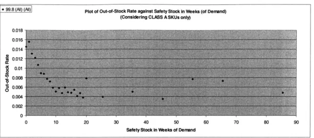
Figure 3.1, Figure 3.2, Figure 3.3 and Figure 3.4 show the exchange curves between OOS rate and safety stock in weeks for CLASS A, CLASS B, CLASS C and New SKUs

respectively. Note that the weights are not the same for all points since the number of corresponding observations varies from point to point. Refer to Appendix A for the data.

In general, the OOS rate decreases as the amount of safety stock increases, which is not a surprise. The "smoothness" of the curves, however, is rather remarkable.

There are three interesting results. The first is that for CLASS B and CLASS C SKUs, the curves flatten off at out-of-stock rates that correspond to their respective service level

targets. CLASS B has a service level target of 99.5%, which corresponds to an OOS rate of

0.005; CLASS C has a service level target of 99.0%, which corresponds to an OOS rate of 0.010.

The second is that for CLASS B and CLASS C SKUs, the out-of-stock rate that corresponds to zero weeks of safety stock is exceptionally low. The number of

observations with zero weeks of safety stock is small but not insignificant - about 12,000

and 160,000 for CLASS B and CLASS C respectively, which translates to approximately 5 and 62 SKU equivalents respectively. (In the data base, for each SKU we have approximately 2500 observations as we have one observation for each of 11 weeks for each of 233 stores.) Also most of these observations have exactly zero safety stock (i.e. zero

SYS.SS and zero MP) - about 9,400 and 159,000 for CLASS B and CLASS C respectively. Though we do not know for sure the reason for this exception, it is possible that these observations correspond to items that are being discontinued; their safety stocks have been cut to zero but still have some inventory on hand.

The third is that for a given amount of safety stock in weeks, the OOS rate for CLASS A is lower than that of CLASS B, which in turn is lower than that of CLASS C. This might be because CLASS C items have a smaller demand rate than CLASS B and as such, its demand is relatively more variable. The same comparison can be made between CLASS B and CLASS A items

* 99.8 (Al) (NI) _{Plot of Out-of-Stock Rate against Safety Stock In Weeks (of Denand)}

(Considering CLASS A SKUs only)

0.018 0.016 0.014 e0.012 0.01 0.008 0.004 0.006 0 0.004 0.002 0 0 10 20 30 40 50 60 70 80 90

Safety Stock In Weeks of DeMnand

Figure 3.1: Plot of OOS rate against WEEKS.SS for CLASS A items

+ () () Plot of Out-of-Stock Rate against Safety Stock in Weeks (of Denand) (Considering CLASS B SKUs only)

0.025 0.02 0.015 0.01 0 0.005 0 0 10 20 30 40 50 60 70 80 90

Safety Stock in Weeks of Denand

S99 (All) (Al) _{Plot of Out-of-Stock Rate against Safety Stock In Weeks (of Demand)}

(Considering CLASS C SKUs only) 0.035 0.03 0.025 0.02 0.015 0 0.01 0.005 0 0 10 20 30 40 50 60 70 80 90 Safety Stock in Weeks of Demand

Figure 3.3: Plot of OOS rate against WEEKS.SS for CLASS C items

* 99.2 (AM) (AI) Plot of Out-of-Stock Rate against Safety Stock in Weeks (of Demand) (Considering New SKUs only)

0.035 0.03 0 0.025 0.02-0.015 0 0.01 0.005 0 0 10 20 30 40 50 60 70 80 90 100 Safety Stock in Weeks of Demand

Figure 3.4: Plot of

OOS

Figure 3.1 which gives the plot for CLASS A SKUs is relatively more scattered because of the smaller number of CLASS A SKUs. CLASS A SKUs constitute approximately 20% of

all SKUs while CLASS B and CLASS C items constitute about 30% and 50% respectively.

The rather scattered plot we see in Figure 3.4 is due to the small number of observations available for new products. We have less than 600,000 observations which translate to approximately 230 SKU equivalents.

3.2 Out-of-Stock Rate and Time Between Orders

We denote the time between orders by TBO and compute it as

TBO = OUTL-ROP

_(3.2)

FC

where OUTL, ROP and FC are the final order-up-to-level, re-order point and seasonalized forecast as given in section 1.2.1. However, because computing the OUTL is rather complex, we estimate equation (3.2) using

TBO = SYS.OUTL -VOP+1

(3.3)

FC

Since the number of observations with active BUYR.MIN, BUYR.MAX and HARD.MAX is small, equation (3.3) provides a good enough estimate for the purpose of our work in this section.

We establish the relationship between time between orders and OOS rate in a similar manner as outlined in section 3.1. Specifically, we first compute the TBO for each and every observation; group observations with similar TBO together; and finally compute the

OOS rate of each group by dividing the number of OOSs by the number of observations,

i.e. by using equation (2.2).

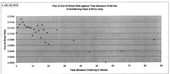
Figure 3.5, Figure 3.6, Figure 3.7 and Figure 3.8 show the exchange curves between the

OOS rate and time between orders in weeks for CLASS A, CLASS B, CLASS C and New

SKUs respectively. Note that the weights are not the same for all points since the number of corresponding observations varies from point to point. Refer to Appendix B for the data.

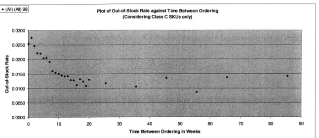
We can see from the figures that for the same time between orders, CLASS A items have a lower OOS rate than CLASS B items, which in turn have a lower OOS rate than CLASS C items. Like in the case of safety stock, this is presumably because the demand for CLASS C and B items is relatively more variable than that for CLASS B and A items, respectively.

S(All) (All) 99.8 Plot of Out-of-Stock Rate against Time Between Ordering (Considering Class A SKUs only)

0.0160-0.0140 -0.0120 + c 0.0100 0.0080 0.0060 0 0.0040 0.0020 0.0000 0 10 20 30 40 50 60 70 80 90

Time Between Ordering in Weeks

Figure 3.5: Plot of OOS rate against TBO for CLASS A items

* (All) (Al) 99.5 Plot of Out-of-Stock Rate against Time Between Ordering (Considering Class B SKUs only)

0.0200 - -7-0.0180 0.0160 S0.0140 Ix 0.0120 0.0100 0.0080 O 0.0060 0.0040 0.0020- -0.0000 0 10 20 30 40 50 60 70 80 90

Time Between Ordering in Weeks

Figure 3.6: Plot of OOS rate against TBO for CLASS B items

Figure 3.7: Plot of

OOS

* (All) (AMI) 99.2 Plot of Out-of-Stock Rate against Time Between Ordering

(Considering New SKUs only)

0.0"0 0.0250 aR T 0.0200 0.0150 0.0100 0 Y 0.0050 0.0000 0 20 40 60 80 100 120

Tirne Between Ordering in Weeks

Figure 3.8: Plot of OOS rate against TBO for New items

Like before, the scattering we see in Figure 3.8 is due to the small number of observations we have for new products, which is approximately only 230 SKU equivalents. On the same ground, the points on Figure 3.5 are relatively more scattered than the points in Figure 3.6

and Figure 3.7.

* (RI) (RI) 99 Plot of Out-of-Stock Rate against Tine Between Ordering (Considering Class C SKUs only)

0.0300-0.0250 1i 0.0200- _ * ra0.0150-0.0100 0.05 0.0050 -0 10 20 30 40 50 60 70 80 90 Time Between Ordering In Weeks

3.3 Out-of-Stock Rate and Normalized Forecast Error

We denote the normalized forecast error by NFE, and define it as

NFE

UNITS.SOLD

-

FC

(34)

FC

where FC as defined earlier is the seasonalized weekly forecast. We note here that (3.4) is not the most widely accepted definition of normalized forecast error. Having

UNITS.SOLD instead of FC as the denominator in (3.4) will give us the more common

definition. However, since many observations have zero UNITS.SOLD, the more accepted definition would face the problem of division by zero.

The relationship between out-of-stock rate and normalized forecast error is established in a similar fashion as outlined in section 3.1. We note that since UNITS.SOLD is rarely negative, then effectively a lower bound on NFE is -1, which corresponds to zero

UNITS.SOLD. However, the NFE often take on a large positive values as many items

have weekly forecasts of less than one unit; for instance, if the weekly forecast were 0.25, and we sell one unit, then NFE = 3.

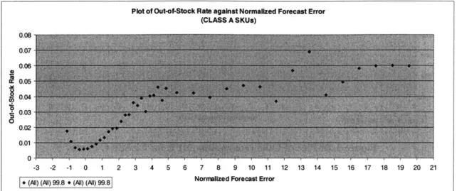
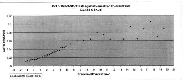
Figure 3.9 to Figure 3.12 show the exchange curves between OOS rate and normalized forecast error for CLASS A, B, C and New items respectively. The results, which show that in general OOS rate increases as normalized forecast error increases is just as we would expect. The data for the plots can be found in Appendix C.

Figure 3.9 shows that the OOS rate corresponding to -1 normalized forecast error is higher than when the normalized forecast error is close to zero. Though at first glance it seems to contradict the general pattern that OOS rate increases as normalized forecast error increases, it is perfectly explainable; a large number of the observations that have -1 normalized forecast error have zero UNITS.SOLD and thus have zero sales because they were out-of-stock and not because there was no demand. The fact that (actual) demand for

CLASS C SKUs is smaller than that of CLASS A SKUs suggests that most of the zero UNITS.SOLD observed for CLASS C SKUs are legitimate, thus explaining why this

pattern is not observed in Figure 3.11. This clearly illustrates the limitation of estimating actual demand using observed demand.

Plot of Out-of-Stock Rate against Normalized Forecast Error (CLASS A SKUs) 0.08 0.07 0.06 W 0.05 0.04 0.03 0 0.02 0.01 0 -3 -2 -1 0 1 2 3 4 5 6 7 8 9 10 11 12 13 14 15 16 17 18 19 20 21

+ (All) (All) 99.8 -(All) (All) 99.8 Nornulized Forecast Error

Figure 3.9: Plot of

OOS

Figure 3.10: Plot of OOS rate against NFE for CLASS B items

Plot of Out-of-Stock Rate against Normalized Forecast Error (CLASS B SKUs) 0.12 0.1 0.08 0.06 0.04 0.02 0 -3 -2 -1 0 1 2 3 4 5 6 7 8 9 10 11 12 13 14 15 16 17 18 19 20 21

Plot of Out-of-Stock Rate against Normalized Forecast Error (CLASS C SKUs) 0.12-0.1 0.08 0.06 0.04 0 0.02 0 -3 -2 -1 0 1 2 * (Al) (Al) 99 * (Ail) (m) 99

3 4 5 6 7 8 9 10 11 12 13 14 15 Normalized Forecast Error

16 17 18 19 20 21

Figure 3.11: Plot of OOS rate against NFE for CLASS C items

Plot of Out-of-Stock Rate against Normalized Forecast Error (New SKUs) 0.16 0.14 0.12 aR 1 0.1 0.08 0.06 0.04 0.02 0 -3 -2 -1 0 1 2 3 4 5 6 7 8 9 10 11 12 13 14 15 16 17 18 19 20 21

* (All) (All) 99.2 * (AlI) (Al) 99.2 Normalized Forecast Error

Figure 3.12: Plot of

OOS

Again, like before, the rather scattered plot we see in Figure 3.12 is caused by the small number of observations available, which we already mentioned in section 3.1 is less than

600,000.

Chapter 4

Out-of-Stock Causes and

Conditions

In this chapter, we will first look at the causes of out-of-stocks in retail stores in general. Following this, we will develop an algorithm to identify the causes behind the out-of-stocks we see in our data. The algorithm also identifies certain conditions under which the

out-of-stocks have occurred. By conditions, we are referring to inventory status or information which may provide insights to the out-of-stock but cannot be defined as being responsible

for it. Finally we will show the results of our algorithm on our dataset.

4.1 General OOS Causes in Retail Stores

[6] reports that between two-third to three-quarter of OOS are caused by problems at the

store level while the remaining are caused by problems upstream in the supply chain. For the out-of-stocks that are caused by problems at the store, almost half of them can be attributed to bad forecasting. Figure 4.1 shows the summary of the various OOS causes in general as given by [6].

Summary of Findings of

OOS

Causes

Figure 4.1: Summary of distribution of

OOS

As noted in [6], the distribution of OOS causes varies significantly between studies. The results shown in Figure 4.1 simply provide an overall picture on the causes.

4.2 Algorithm to Determine OOS Causes

We have developed an algorithm to determine the possible OOS causes using only the information from the dataset. This section will describe the algorithm and provide a discussion on its accuracy and possible pitfalls.

4.2.1 Description of Algorithm

Recall that our dataset is a weekly snapshot of the inventory status of all active SKUs at

233 selected stores over a period of 11 weeks. Because the dataset consists of weekly

snapshots, we are limited in our ability to identify the reasons for any particular out-of-stock occurrence. From the data we have, we can identify the following possible causes-out-of-stock at the DC, causes-out-of-stock at the DC in the prior week, order delayed and

insufficient replenishment. We also keep track of three conditions under which the OOS has occurred. The first is whether any replenishment occurred during the week; the second is the type and extent of forecast error; and the third is on the existence of an inventory

adjustment.

In this section, we denote the store, SKU and week using the first, second and third subscripts respectively. Thus an observation in store i of SKU k at the end of week t is denoted by OBSk . All of the notations we use here have been declared in section 2.1.1.

Out-of-Stock

Given OBSk,,, we declare that it corresponds to an out-of-stock if

IOH , : OUT.POINTIj. (4.1)

OOS at DC

For SKUs that are replenished from the DC, an OOS at a store might be due to the fact that the DC was previously out of stock and a replenishment order has thus been delayed. We have the data on the inventory status of the DC; to determine if the DC was

out-of-stock at week t and/or at the prior week, we check this directly from the data as shown by,

DIOHij 0 (4.2)

DIOH

,

SKUs that are replenished directly by the suppliers via the flow through policy do not hold any stock at the DC; hence, for these SKUs, their OOSs are precluded from the above checks. Another way to look at it is that OOSs that are not flagged as being OOS at DC either have stocks available at the DC or are flow through items.

No Replenishment in Week t

We can identify that no replenishment was received during week t if the number of units sold in the week is less than or equal to the net change in on hand inventory from the prior

week. That is, we conclude that there was no replenishment in week t if the following condition is true:

UNITS.SOLDijt IOHi,, - IOHj, + INV.ADJijt (4.4)

Order Delayed

We can infer from the data that an order was delayed if there was no replenishment in week t, the inventory on hand in the prior week was lower or equal to the re-order point and the lead time was less than 6 days. In order words, we assert that an order was suppose to arrive in week t, but did not, if the following conditions are satisfied:

UNITS.SOLDjt IOH,3

~

IOH ,1 ! ROi,jt (4.5)

LEAD.TIMEi,_

< 6

(4.6)

In using the above criteria to identify an order delay, we are making two assumptions. The first assumption is that an order was placed in the prior week, given that the inventory on hand was at or below its reorder point. The second assumption is that if the lead time is less than 6 days, then any order placed in the prior week should have arrived at the store by the end of the current week; our understanding of Beta's operations indicate that this should be true even if a store has a pick frequency of 1 or 2 times a week.

Inventory Adjustment

We can use the occurrence of an inventory adjustment as an indicator of the store execution performance. An OOS might be due to inventory inaccuracy; an inventory adjustment occurs whenever the store finds an inventory inaccuracy, namely a discrepancy

between its on-shelf inventory and the inventory records. Since the data provides

information on the net inventory adjustment for the week, determining if an inventory adjustment has occurred is straight forward.

Negative Inventory Adjustment if INV.ADJJt <0, (4.7)

Positive Inventory Adjustment if INV.ADJjt >0, (4.8)

Insufficient Replenishment

We declare that there was insufficient replenishment if an order was received and the order received was less than the expected order quantity. This event occurs if the following two equations are satisfied.

UNITS.SOLDJ , > IOH,41 - IOHij~ + INV.ADJiJ, (4.9)

UNITS.SOLDj

<

''-,j x SP,,-

NET.CHANGEI,

(4.10)

where SP denotes the Ship Pack for the SKU,

[.]

integer and NET.CHANGE denotes the net change in on hand inventory, which is given as

NET.CHANGEj = IOH,,, - _{IOH,+ INV.ADJ ,} (4.11)

Thus, equation (4.9) signifies that a replenishment was received in week t while (4.10) indicates that the amount received was less than what was expected. The term in brackets is the number of ship packs that would need to be ordered to bring the inventory up to the order -up-to level.

Forecast Error

An OOS might be due to a forecast error, especially when demand exceeds the forecast. We characterize the types and extent of the forecast error in week t as follows,

Non-positive error if FEi, 5 0,

Small positive error if _{0 < FEi,, 5 FC,,}

Medium positive error if FC,₁ < FE,'' 5 2 FC,,

Large positive error if FE , > 2FCI,, ,

(4.12) (4.13) (4.14) (4.15)

where FC is defined in section 2.1.1, and denotes the seasonalized weekly forecast, and FE denotes the forecast error, which is computed as

SELt

UNITS.SOLD ,

-

FC(4

We categorize the positive forecast errors into small, medium and large based on the relative size of the error. In particular we use the square root of the weekly forecast as the basic unit for scaling the forecast error. This choice of scale is arbitrary.

4.2.2 Discussion on Algorithm Accuracy

Given that the dataset we have provides us with only snapshots of the weekly inventory status, the accuracy of our algorithm is thus limited. Here, we discuss two errors that our algorithm might make when checking for order delay.

False Positives on Detecting Order Delayed

By false positives, we refer to OOS that were not caused by a delay in the order but yet this

condition was flagged otherwise by our algorithm. For our algorithm, we assume that if a store places an order on Saturday, then this order will normally arrive by the following Saturday. It is possible that this might not be true. For instance, if the store has a pick frequency of once a week, it is conceivable that the replenishment lead time is such that the order placed on Saturday cannot be shipped as part of the one weekly replenishment for the store. Technically, an order which fails to arrive at the store after its lead time has lapsed because it has legitimately missed the replenishment day of the store cannot be

classified as being caused by an order delay. However, given that over 70% of the

observations have a lead time of two days or less and that more than 80% of the stores are replenished at least twice a week, we expect the number of false positive to be small.

False Negatives on Detecting Order Delayed

There are three ways for false negatives to occur. By false negatives we refer to OOS that were caused by a delay in the order and we were not able to detect this order delay this with our algorithm.

The first case happens when the lead time is greater than 6 days. By default all OOSs for SKUs with a lead time of 6 days or more would not be flagged as being caused by an order

44

delay. Approximately 28% of the observations have a lead time of 6 days or more, of which more than 85% corresponds to SKUs that are on flow-through replenishment from the supplier.

The second case occurs when the inventory position hits the reorder point after Saturday of week t-1 but before Saturday of week t and the time between reordering and Saturday of week t is less than the lead time. By making the assumption that demand is Poisson, then with the information on the total demand of the week we will have a conditional Poisson distribution, which essentially is the same as having the observed demand uniformly distributed over the week. Thus, for a given OOS observation, we might observe that an order was delayed if the order had been placed (say) by Monday of week t; given the observed demand for the week and the assumption of Poisson demand, we could find the probability that an order was delayed in arriving by the end of week t.

The third case occurs when there are multiple replenishment orders outstanding and one or more of these are received in week t. According to our specification, because a

replenishment was received during week t, we do not associate an order delay to this OS;

however, the fact that an order was received in week t need not rule out the possibility that there is an outstanding delayed replenishment order.

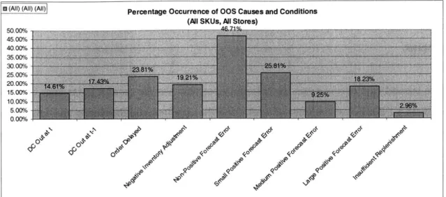
4.3 Results

Figure 4.2 gives the overall picture of the conditions and causes surrounding the out-of-stocks. We note that for each OOS we associate all of the conditions and causes that are satisfied. Thus each OOS might have several conditions or causes. We see that for 86% of the OOSs, either there was inventory at the DC in week t or they are flow through items; for 8 3% of the OOSs, either there was inventory at the DC in week t-1 or they are flow

through items. The percentages corresponding to the four types of forecast error sum up to a hundred. Figure 4.3 shows the same picture but with a breakdown by SKU CLASS. Refer to Appendix D for the data.

* (All) (All) (All) Percentage Occurrence of OOS Causes and Conditions

Percentage Occurrence of OOS Causes and Conditions

(All SKUs, All Stores)

m (All) (All) (All)

50.00%'6 45.00% 40.00% 35.0006 30.00% 25.00% 20.00%/ 15.00% 10.00%/0 5.00% 0.00% -0 J 0 Z

de'Al

Figure 4.2: Plot of percentage occurrence of

OOS

Percentage Occurrence of OOS Causes and Conditions (Split by SKU Class, All Stores)

70.00% 5000CLASS C 40.0 H mCLASS B 40.00%/ 30.00 ! o CLASS A 20. New 10.000/0 0 00 .40 40 0~ NO'~ 40 40 0 40 .10

Figure 4.3: Plot of percentage occurrence of

OOS

CLASS

To get a consolidated view of the OOS causes and conditions, we selected a few combinations of OOS conditions and causes that are most pertinent and compare their relative frequencies. The results are shown in Figure 4.4 and Figure 4.5. Out-of-stocks are classified as "No Other" if the only condition that we could identify for the OOS was that of the forecast error. "Only Neg Adj" and "Only Order Delay" correspond to the OOS for which we could detect only "negative inventory adjustment" and "order delayed"

46

.40 _.00N,

.40

0 4I