The influence of active region information on the prediction of solar flares: an empirical model using data mining

(1)

HAL Id: hal-00318009

https://hal.archives-ouvertes.fr/hal-00318009

Submitted on 22 Nov 2005

HAL is a multi-disciplinary open access

archive for the deposit and dissemination of

sci-entific research documents, whether they are

pub-lished or not. The documents may come from

teaching and research institutions in France or

abroad, or from public or private research centers.

L’archive ouverte pluridisciplinaire HAL, est

destinée au dépôt et à la diffusion de documents

scientifiques de niveau recherche, publiés ou non,

émanant des établissements d’enseignement et de

recherche français ou étrangers, des laboratoires

publics ou privés.

The influence of active region information on the

prediction of solar flares: an empirical model using data

mining

M. Nuñez, R. Fidalgo, M. Baena, R. Morales

To cite this version:

M. Nuñez, R. Fidalgo, M. Baena, R. Morales. The influence of active region information on the

prediction of solar flares: an empirical model using data mining. Annales Geophysicae, European

Geosciences Union, 2005, 23 (9), pp.3129-3138. �hal-00318009�

(2)

Annales Geophysicae, 23, 3129–3138, 2005 SRef-ID: 1432-0576/ag/2005-23-3129 © European Geosciences Union 2005

Annales

Geophysicae

The influence of active region information on the prediction of solar

flares: an empirical model using data mining

M. N ´u ˜nez, R. Fidalgo, M. Baena, and R. Morales

Department of Computer Sciences, Universidad de M´alaga, Campus de Teatinos s/n, M´alaga 29 071, Spain Received: 14 February 2005 – Revised: 5 May 2005 – Accepted: 20 June 2005 – Published: 22 November 2005

Part of Special Issue “1st European Space Weather Week (ESWW)”

Abstract. Predicting the occurrence of solar flares is a chal-lenge of great importance for many space weather scientists and users. We introduce a data mining approach, called Be-havior Pattern Learning (BPL), for automatically discover-ing correlations between solar flares and active region data, in order to predict the former. The goal of BPL is to predict the interval of time to the next solar flare and provide a con-fidence value for the associated prediction. The discovered correlations are described in terms of easy-to-read rules. The results indicate that active region dynamics is essential for predicting solar flares.

Keywords. Solar physics, astrophysics and astronomy (flares and mass ejections; instruments and techniques; gen-eral or miscellaneous)

1 Introduction

One of the most important aspects in the study of space weather is related to avoiding the consequences of space weather events either by system design or by efficient warn-ing and prediction systems (Feynman and Gabriel, 2000; Koskinen et al., 2001). Some of the users of these predic-tions are telecommunicapredic-tions operators, the electric power industry, space agencies and defense departments.

Space weather events are strong solar events, like CMEs, that affect the virulence of solar wind and this, in turn, af-fects the geoelectric field, which may produce, for exam-ple, different voltages between the grounding points of two transformers, and therefore may produce a current in the power transmission line connection between the transform-ers. Other events, such as solar flares, may affect space-craft/aircraft passengers’ health and space technology. Sub-stantial progress has been made in understanding the rela-tionships between CMEs, flares and the geomagnetic distur-bances of those phenomena (Kahler, 1992). It is clearly seen

Correspondence to: M. N´u˜nez

(mnunez@lcc.uma.es)

that the prediction of all of these major solar events is indeed a space weather topic of vital significance.

Several methods, classified as theoretical, statistical and empirical, may be applied for forecasting physical phenom-ena. Theoretical models must be embedded in data mining or data assimilation codes for predicting solar events because of the large complexity of the problem (Hochedez, 2004). Sta-tistical methods (Boffeta, 1999; Wheatland, 2001; Moon et al., 2001) are used extensively for predicting the probability of the occurrence of a solar flare on the next day. Wheatland presented a method for flare prediction using only observed flare statistics and the assumption that flares obey Poisson statistics in time, and power-law statistics in size. The per-centage probabilities are based on the number of flares pro-duced by regions classified using the McIntosh classification scheme (McIntosh, 1990) during cycle 22. This approach is followed by the Flare Prediction System of the NASA God-dard Space Flight Center1. Some statistical methods take dynamic flare data and static active region data as input, but none of these methods takes into account data about the dynamics of the active region (i.e. the area, the number of sunspots, magnetic classification of the active region).

On the other hand, current empirical methods, like neu-ral networks, decision trees, Bayesian networks and Hid-den Markov Models, can predict the next value of a vari-able based on the short-term conditions of several varivari-ables, but they do not predict the interval of time to a future event, nor were these methods designed to manage mid- and long-term dependencies. If temporal patterns are to be discov-ered, the variable space of these methods must be increased by a factor that is the number of analyzed past time steps (Ngo et al., 1995). Complexity becomes particularly prob-lematic as researchers seek to build models with a longer number of time steps (Ngo et al., 1995). In empirical meth-ods that do analyze past information, such as the temporal series ARMA-models (Box and Jenkins, 1976), the output

Yt for any time interval can be determined from the input

(3)

3130 M. N´u˜nez et al.: The influence of active region information on the prediction of solar flares

values for a small number of time steps in the recent past

Yt=φ1Yt −1+. . . + φpYt −p+θ1Wt −1+. . . +θt −qWt −q, where φ and θ are unknown coefficients measuring the influence of past variables on Yt; Wt −1, Wt −2,. . . are the error terms, p

and q are the number of autoregressive terms and moving average terms.

Other empirical methods have been proposed recently to analyze temporal sequences and discover sequence patterns (Manila et al., 1997; Srikant and Agrawal, 1996). Basically, input data can be viewed as a sequence of events, where each event has an associated time of occurrence. Currently, there are expert systems, with knowledge acquired from hu-man experts, which may predict communication alarms that are the expected consequences of a current problem. The automatic generation of those expert systems is a valuable tool. When discovering episodes in a network alarm log, the aim is to find relationships between the alarms. Such relationships can then be used in an analysis of the incom-ing alarm stream, for example, to better explain the problem that causes the alarms, to suppress redundant alarms, and to predict severe faults. However, these methods have the fol-lowing limitations: they only analyze the sequence of events; they cannot analyze correlation with dynamic variables out-side the event sequence, i.e. in the present study they would not discover correlations with the dynamics of the active re-gion. For this reason, a new empirical method for predicting events was introduced recently for predicting alarms from a history of communication events and configuration attributes of the monitored equipment. This event-oriented data min-ing method, called BPL (Núñez, 2000a; Núñez et al., 2002, 2004a) has also recently been used for predicting solar flares, particularly M-class flares – another event-oriented problem – (Núñez et al., 2004b), and BPL preliminary results are ex-plained in the present paper.

This paper describes how BPL is trained to formulate a model in order to predict the interval time to the next M-class flare and provide a confidence value for the prediction; the frequency of this class of solar flare is appropriate for our methods. The input of BPL consists of two data sets: a log of solar flare data and a log of active region data. Instead of in-creasing the variable space for every past time step, as current empirical methods do, BPL analyzes the temporal distances and the number of events as new variables. BPL studies frequent correlations between temporal distances of events, bursts of past events and information outside the event se-quence (i.e. the variables that describe the active region dy-namics). The output of the method is a set of understandable rules that predict the approximate interval time of occurrence of a target event with a confidence level in that prediction. In practice, BPL is an online component, which can estimate a prediction at a given time, and later update the prediction as time passes by.

BPL discovers understandable knowledge which helps sci-entists to recognize known patterns or to discover new ones. Scientists may give rapid feedback to the model construction because they can read the discovered knowledge more eas-ily than with “black box” models (for example, neural

net-works models). Another difference is that BPL also analyzes the information outside the sequences. However, the main difference with all current methods is that BPL predicts the approximate interval time to the next target event, instead of predicting its next value or a probability of occurrence within a fixed period of time.

In the present study, BPL discovered general patterns, which are supposed to be valid for every active region during the analyzed time interval (2003), in terms of understandable rules. BPL found temporal dependences with past events (i.e. past C- and M-class flares) from 1 min to several days. It also found that the dynamic variables (i.e. the growth of the area, the magnetic classification, the longitudinal extent and the growth in the number of sunspots) of the observed systems (the active regions) are important to predict eruptive events (M-class flares).

This paper is organized as follows: Sect. 2 explains the BPL data mining method. Section 3 describes the exper-imental results for predicting solar flares, Sect. 4 presents limitations of the method and proposes future directions, and Sect. 5 presents the conclusions.

2 The BPL event-oriented method

The BPL method discovers temporal patterns by taking into account the observed events, the static attributes of the ob-served systems, and their environments. In this field of ap-plication, we consider the Sun to be an environment, and the different active regions as systems. Both the Sun and the active regions have attributes that describe them in every in-stant of time. For the experimentation presented in this paper we did not include data about the environment of an active region (e.g. total sunspot numbers in the Sun) because we wanted to concentrate our research on the influence of the active region information in the prediction of solar flares. We want target events (such as M-class flares) to be predicted by an understandable model. The events are triggered from ac-tive regions. The information that comes from the Sun and the active regions is the input for BPL.

We consider a continuous time model. An event may hap-pen at any arbitrary point in time. Temporal patterns are used to predict target events. These patterns are explained in an understandable way, called behavior rules, which may con-tribute to an understanding and explanation of the problem.

The main strategy of BPL is: 1) building training labeled examples as events (i.e. flares) occur, and 2) constructing re-gression trees from the training examples, thus:

1. BPL takes “a snapshot” of the behavior of a situa-tion, building a training example that is characterized by all static and dynamic attributes of the phenomenon (i.e. area of an active region) at that time and adds new attributes to this snapshot. “Repetition of events”, which is the frequency of past events during a latency window (i.e. a burst of 12 B-class flares in the last 5 h), and the “age” of past events, which is the distance from

(4)

M. N´u˜nez et al.: The influence of active region information on the prediction of solar flares 3131

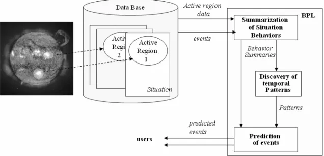
Figure 1. Behavior Pattern Learning (BPL) processes.

Fig. 1. Behavior Pattern Learning (BPL) processes.

the past events (i.e. the last time an M-class flare oc-curred). Each example is labeled with a number: the temporal distance from the time of the snapshot to the next future target event (i.e. 6.8 h for the next M-class flare).

2. BPL takes these training examples and uses them to for-mulate a regression tree. Regression trees may be seen as a set of prediction rules. Each prediction rule gener-ated by BPL has a confidence level. The confidence is the proportion of training cases in which the prediction rule worked well given all training cases that fulfill the antecedent of the rule. It suggests how much a user can trust the corresponding rule.

2.1 Background

In order to analyze the possible consequences of an event, the following natural assumptions are made: an event could be a consequence of some temporal correlation of past events, the static and dynamic characteristics of the observed system and the static characteristics of the environment; on the other hand, an event could have an effect in the future for a limited period of time, which is the Latency Window (section 2.2 summarizes how BPL calculates the latency windows). As a result, two observed systems in the same state, situated in two different environmental conditions, behave differently. For this reason BPL also draws from the events and the static information of the system and its environment.

This section first introduces the BPL process before ex-plaining it formally in Sect. 3. In the field of communica-tions, for instance, a fault in a device may produce a sequence of events in the short- and/or mid-term generated by the as-sociated devices that detect faulty behaviors.

Figure 1 shows the two processes of BPL. The first pro-cess is the “summary of situation behaviors”. A situation

is made up of an “observed system” and its “environment”. Both are characterized by dynamic attributes and static at-tributes. A change in the value of a dynamic attribute, as well as the time in which this change takes place, is regis-tered as an event. An event schedules the construction of several behavior summaries in the future during its latency window.

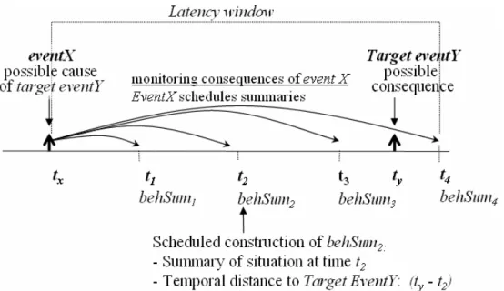
Figure 2 illustrates the way BPL monitors the conse-quences of “eventX”, scheduling four behavior summaries during a time interval. This time interval is the period of time during which “eventX” is supposed to affect the future. BPL constructs summaries with the static and dynamic attributes of the system and its environment, as well as new features from the events, such as the duration of current event values, repetitions of an event in a period of time, and the age of past events.

The second process is the “discovery of temporal pat-terns”. Chaotic systems are characterized by a continuous increment of the entropy. BPL searches for these intervals by applying a multivariate technique that uses the growth of discovered patterns as a heuristics indicator of chaos. If the number of new prediction rules does not grow signifi-cantly, then a non-chaotic interval is detected; otherwise, a chaotic interval is assumed. In experiments with solar flares, we never detected non-chaotic intervals. More research has to be done to demonstrate this heuristic. If the prediction is to be made in a chaotic interval, then temporal patterns are constructed by taking into account only the behavior sum-maries in that chaotic interval. If the prediction is to be made in a non-chaotic interval, then the temporal patterns are constructed by taking into account the whole history of non-chaotic behavior summaries. Temporal patterns show: the preconditions (static and dynamic) for a target event to happen, the next expected time interval of occurrence, and the support of the pattern. This process constructs a set of

(5)

Figure 2. Monitoring the consequences of an event.

Fig. 2. Monitoring the consequences of an event.

temporal patterns for predicting a target event. This set of patterns is called a behavior tree (see Fig. 3).

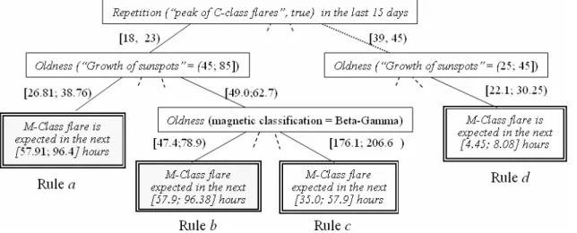
Figure 3 shows a portion of the predicted rules discovered by BPL. Another more natural representation for the a and

drules shown in Fig. 3 are: Rule a:

IF <The rate of C events is> = [18; 23] in the last 15 days,

<Last time the growth of sunspots reached the band [45; 85] was> = [26.81; 38.76] h

THEN an M-class flare is expected in [57.91; 96.4] h (100% confidence).

Rule d:

IF <The rate of C-class flares> = [39; 45] in the last 15 days,

<Last time the growth of the area reached the band [25; 45] was> = [22.1; 30.25] h

Once prediction rules are created, event prediction may be made. The prediction process receives a behavior summary (without distance to the target event) and moves it down the behavior tree to predict an event.

We empirically validated BPL prediction accuracy with nonlinear systems described by differential equations: the Double Well Oscillator and the Lorenz system (N´u˜nez et al., 2002).

2.2 Basic concepts related to BPL

Before summarizing the algorithms, we need to define the concepts involved.

2.2.1 Observed system

An observed system is described by (a) static attributes: sSA1,. . . , sSAa, and (b) dynamic attributes: sDA1,. . . , sDAb, namely, a vector with a+b components: ObservedSys-tem=(sSA1 . . . , sSAa, sDA1,. . . , sDAb). An environment, in a similar way to a system, has c static attributes and d dynamic attributes, that is to say, a vector with c+d compo-nents: Environment=(eSA1, . . . , eSAc, eDA1, . . . , eDAd ). For each static attribute, sSAi, eSAi, and for each dynamic attribute, sDAr, eDAs, the domains of values are defined for: sSADi, eSADj, sDADr, eDADs, respectively. In our prob-lem, each active region is an observed system. As mentioned above, we did not include environmental data.

2.2.2 Situation

In general, a situation is composed of the observed “system” and its environment. We will have a group of situations that we identify from now on with positive integers: situation =

{1, 2, 3, . . . , n}, understanding that for each sit= 1,. . . , n , we have the observed system sit, and its environment. The inte-ger sit that identifies the situation is the active region number given in the NOAA files.

2.2.3 Events

The observed events describe the changes observed at an in-stant t and a situation k. The observed events will be generi-cally called events. An observed event will be characterized only by:

– System identifier (Active Region identifier)

– pe=(f, v) a possible event type, where f is the name of the static or dynamic attribute and v is its new value (e.g. “Peak of C-class flare”, true)

(6)

Figure 3. A behavior tree. A rule is the conjunction of the conditions from the leaf to the root.

Fig. 3. A behavior tree. A rule is the conjunction of conditions from the root to the leaf.

– t (indicating the instant in which the attribute f changes its value to v).

For the flare problem described in this paper all solar flares were “system” events. However, environmental events could have been included if more sophistication and complexity were needed (i.e. for analyzing the active region n, BPL could include the flares of the active region n+1 and region

n-1).

2.2.4 Target event type

A target event type te is a possible event of the system whose occurrence is to be predicted. For the problem presented in this paper the target event is the M-Class event.

2.2.5 Events associated with target events

We say that the possible event ae is associated with a target event te, if ae may cause te in the future, i.e. they are tempo-rally correlated.

2.2.6 Latency Window

For each pair (target event te, associated event ae), we de-fine their latency window LW (te, ae) as the interval of time in which the target event te may happen as a consequence of the occurrence of ae. BPL makes an automatic estima-tion of latency windows by reading the temporal distances between associated events ae and their next target events te in the event history log, and calculating the mean µ and the standard deviation σ . Thus, the latency windows LW(te, ae) could have been heuristically established as µ+kσ . By de-fault k=3. In this problem, the Latency window has been set manually to a fixed value (15 days) because the length of the sequence is comparable with the temporal distances between M-Class flares. If we had to predict C-class flares, whose temporal distances are very short compared with the life of an active region, the automatic calculation of the La-tency Windows would be enabled, as stated in this section.

2.2.7 Behavior summaries

A behavior summary bs is the description of a situation at an instant of time. A situation is determined in terms of the char-acteristics of an observed system and its environment in the present, past, and future. A behavior summary is identified by: situation(bs), the targetEv(bs) and constructionTime(bs) . A behavior summary will have the following data:

– the values of the static attributes of the observed system and its environment,

– the values of the dynamic attributes of the observed sys-tem and its environment at constructionTime(bs), – the values of the calculated attributes:

– duration aei(bs,aei) | oldness aei(bs,aei) – repetition aei(bs, aei),for i = 1 to |AEi|,

– the numeric class: the Distance te(bs) from bs construc-tion time, say, tbs, to the time of the next target event te, say, tt e., i.e. these tt e−tbs.

Note that all these values are available from the event log, and depend on the latency windows.

2.3 Description of BPL processes

The construction of each behavior summary is carried out gradually by means of the analysis of the events that occur in the learning system.

2.3.1 Overall learning process

Table 1 shows the overall learning BPL algorithm. From input BPL first builds BS=Uj bsj: state(bss)=“labelled” by applying the function

SummarizationOfSituationBehav-ior (EventLog, TE). Then, we build a prediction model

us-ing the function DiscoveryOfTemporalPatterns(BS, TE) with the purpose of learning to predict the occurrence of the target

(7)

Table 1. Summary and discovery algorithm of BPL method.

Input: EventLog: The set of events from active regions TE: The target event to be predicted

Output: BS: The resulting set of behavior summaries DiscoverLatencyWindows(EventLog, TE)

For each event ei∈EventLog:

ScheduledBS=MultiScheduleBS (ei)

PendingBS=PendingBS ∪ MultiUpdateBS(ScheduledBS)

If ei∈TE Then BS = BS ∪ MultiLabelBS (PendingBS, ei)

EndFor

IdentifyChaoticBS (BS, te) rtr= Regression(BS,TE).

btr= RefineBehaviourTree(rtr)

Return PredictionModel= Umbtm

events te. Therefore, for TE={te1, . . . , ten}we will have |TE| behavior trees bt1, . . . , bt|T E|.

In general terms, the algorithm in Table 1 shows the fol-lowing operation. It takes as input a set of events from active regions in accordance with previous nomenclature, as well as a set of target events that are what we will aim to pre-dict in the operational prepre-dicting phase. The first step is to calculate the latency windows of each of the events with the programmed objectives and subsequently process the events one by one, programming behavior summaries, completing them with the state that the situation has at that time and cal-culating the values of the calculated attributes. Only when a target event arrives are the pending summaries labeled and stored for future processing. Once the file of events has been processed, chaotic regions are identified in order to be dealt with before generating the prediction model.

Below (in Sect. 2.3.2) we detail the procedures related to with the generation of summaries and to the creation of pre-diction models (Sect. 2.3.3).

2.3.2 Summary of situation behaviors

The DiscoveryLatencyWindows procedure automatically calculates and associates the different latency windows of each event (ei) with the target event (TE):

LW(ei,TE)=mean(distances(ei,TE))+ k*standard deviation (distances(ei,TE)),

where distances (ei,TE) are the distances from all occur-rences of event ei to the nearest TE in the future, and k=3.

We define MultiScheduleBS as the procedure that sched-ules behavior summaries when an event e arrives. This func-tion schedules a fixed number of bs values (i.e. 10), starting from the occurrence time of the event (time) to a time equal to time+LW(e, te). This function will not create a bs if it is very close (less than a fixed threshold) to an existing bs. This function initializes the bs values with values of static attributes. An example has been shown in Fig. 2.

We define MultiUpdateBS as the procedure that fills dy-namic and calculated attributes of the behavior summaries based on event e. The strategy for doing this efficiently

is to have only one bs with the state “updating-token”, ab-breviated as bstoken, for each situation. If the event time

t <constructionTime(bstoken), then the dynamic and

calcu-lated attributes corresponding to the associated event ae are updated only in the bstoken, taking constructionTime(bstoken)

as the parameter T for applying the functions described in Sect. 3.1.6. But if t≥constructionTime(bstoken), the

to-ken is then passed from bs to bs until t <construction

Time(bstoken). Then, the bstoken can be updated according

to event e. During the token pass, each bstoken is updated

and its state changes to “updated-and-not-labeled”, indicat-ing that they are waitindicat-ing for the arrival of future target events to be labeled.

We define MultiLabelBS (sit, te) as the procedure that fires when a target event te has arrived. This procedure labels the

scheduled behavior summaries bsi of a situation sit with the time of occurrence of te–constructionTime(bsi).

2.3.3 Regression of temporal distances

According to Table 1, we define IdentifyChaoticBS () as the procedure that “detects” and “filters” the bs values. This function detects a chaotic interval when there exists a contin-uous increment of patterns equally supported by examples. If chaotic intervals are detected, this function sets the chaoticity of these bs values to “recentlyChaotic”. If a “non-chaotic” interval is detected, this function sets the “chao” of these bs valuesto “non-chaotic” and deletes every bs whose state is

“recentlychaotic”. The result of this procedure is that the BS

has only non-chaotic or recently chaotic bs values. Note that, if there are bs’swith state “recentlychaotic”, it means that the last observed interval of the bs values is chaotic. Then, BPL will construct temporal patterns only from the most re-cent chaotic interval. If the last observed interval of bs is non-chaotic, BPL will construct the patterns by taking into account the whole history of the surviving bs values.

We define BehaviorTree as the function that grows a re-gression tree for predicting the distance te. Then it refines this regression tree into a behavior tree, adding information about the latency windows used to inner nodes of the tree and also to the leaves, distance te(bs). Experimentation on Sect. 3 uses EGR (Economic Generalizer for Regression, N´u˜nez, 2000b) as a regression tree construction algorithm. EGR constructs a model for forecasting a numerical variable from other numerical and categorical variables. EGR grows shorter regression trees than CART (Breiman, 1984), an-other (well-known) algorithm to construct classification and regression trees.

3 Experimental results

In order to discover temporal patterns among solar flares and their source active regions, we fed BPL with a log of so-lar fso-lares which occurred during 2003 and were observed by GOES satellites. Information is in the database of the NOAA, Space Environment Center.

(8)

3.1 Description of the data

Two types of information were taken into account for dis-covering temporal patterns: active region data and solar flare data. In the present study every active region is considered as a situation (see Sect. 2.2). The identifier of the situation is the NOAA number of the active region. The next subsections describe the solar flare and active region data.

3.1.1 Solar flare data

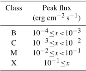
We took into account four classes of solar flares: B, C, M and X of the Solar Event Reports [ESE] of NOAA2. Table 2 shows the classification of solar flares according to the peak flux in the X-ray range. We did not consider the A-class because they have a very low peak flux as compared to the other four classes.

There are two concepts that are integrated in single events: the solar flare class and the temporal phase of a solar flare. An event can be in one of the three possible temporal phases: begin, peak and end. BPL event captures the change as a sin-gle attribute, then there is a need to integrate the flare class and temporal phase. We used Boolean attributes for sum-marizing this information. The beginning of the i-class flare generates an event record with the following information: [RegionId, “Begin of i-class flare”, value, time].

When the i-class flare reaches the maximum flux, another event record is generated:

[RegionId, “Peak of i-class flare”, value, time].

When the i-class flare ends, another event record is gener-ated:

[RegionId, “End of i-class flare”, value, time].

In the above statements “RegionId” is the NOAA number of the active region; i is the solar flare class: B, C, M, X (i.e. “Begin of M-class event”); “value” is a Boolean value which is always true for these event types in this problem; and “time” is the Coordinate Universal Time of occurrence of the begin, peak or end of the solar flare. Since there are four solar flare classes (B, C, M, X) and three temporal phases (begin, peak and end), the number of event types associated with solar flares that we took into account was twelve.

During 2003, the number of X, M, C and B-Class flares recorded was 20, 160, 1315 and 899, respectively; however, we did not process flares that lacked information about the corresponding active region identifier. For this reason, the number of flares taken into account by BPL was 16, 143, 361, and 890, respectively.

3.1.2 Active region data

The active region data has been extracted from the Solar Re-gion Summary [USAF/NOAA SRS] of the USAF/NOAA3,

2_{http://sec.noaa.gov/ftpdir/indices/events/README} 3_{http://sec.noaa.gov/ftpdir/forecasts/SRS/README}

Table 2. Solar flare classification scheme according to the Peak flux

in X-rays. (0.1–0.8 nm).

Class Peak flux (erg cm−2s−1)

B 10−4≤x<10−3 C 10−3≤x<10−2 M 10−2≤x<10−1 X 10−1≤x

which shows the evolution of the active region variables. The Solar Region Summary is a daily report, compiled by NOAA, about the active solar regions observed during the preceding day. It contains a detailed description of the active regions visible on the solar disk, on a given day. The characteristics for each active region are compiled from approximately half a dozen observatories that report to the SEC (Space Environ-ment Center at NOAA) in near-real time. The sunspot counts are typically higher than those reported in non-real time by the Sunspot Index Data Center (SIDC)4, Brussels, Belgium, and the American Association of Variable Star Observers5.

For predicting events we took into account all the at-tributes of the active region registered in the Solar Region Summary, which are:

– The active region number assigned to a sunspot group during its disk passage;

– The Carrington longitude of the group;

– The total area of the group in millionths of the solar hemisphere;

– The modified Zurich classification of the group; – The longitudinal extent of the group in heliographic

de-grees;

– The total number of visible sunspots in the group; – The magnetic classification of the group.

We also added new attributes regarding the derivative of four continuous attributes:

– Growth of the area;

– Growth of the Carrington longitude; – Growth of the Longitudinal extent; – Growth of sunspot number.

We also converted the evolution of the attributes into events as follows: for the categorical attributes, we generated an event record every time the attribute changed. For continuous attributes we generated seven bands, with the five inner bands of equal size. An event record was generated every time the continuous attribute reached a band.

4_{http://sidc.oma.be} 5_{http://www.aavso.org/}

(9)

3.2 Experimentation

We compared this predicted time interval made by BPL with the real time of occurrence of the event. For measuring er-ror we used Relative Mean Square Erer-ror (RMSE), a typical measure used in regression (Breiman et al., 1984). It is rela-tive because it is the ratio between the error of the analyzed predictor and the error of the naive mean predictor. If RMSE is greater than 1, this means that the predictor is worse than a naive predictor that always predicts the median of values. In our problem, the values represent temporal distance to the next occurrence of a target event.

Now we will describe the RMSE estimation formulas. Let L be a learning sample (X1, y1), . . . , (Xn, yn), where, for time series methods, Xi is the time of observation ti and, for multivariate methods, like BPL, Xiis the vector of descriptor values of the learning example i at time ti; yi is the numeri-cal class of the example i. One wants to use L both to con-struct “predictor(X)” and to estimate its error E(predictor). The V-fold cross-validation (Weiss and Kulikowski, 1991), estimate E(predictor) comes from dividing L into V subsets

L1, . . . , LV, each one containing a learning sample of size

n/2 of consecutive observations and a testing sample with the next V% observations. Then the typical cross validation formula is used: E(predictor) = 1 N X v X (Xn,yn)∈Lv (yn−predictor(v)(Xn))2,(1)

Where ynand predictor (Xn) are the real and predicted tem-poral distance to the next occurrence of a target event after the observation Xn,and v is the number of subset to test. The mean square error depends on the scale in which the response is measured. For this reason, a normalized measure of accu-racy that removes the scale dependence is often used. Let

µ=(1/N)6nyn, and E∗(µ)=(1/N) 6n(yn−µ the na¨ıve mean predictor, then the sequential cross validation estimate is:

RMSE(predictor) =E(predictor)

E∗_(µ) . (2)

In order to use RMSE in a sequence, we used a sliding win-dow of size V/2 for delimiting the training set and other set of size V, immediately after the training set, to calculate the RMSE formulae explained above. These training and testing windows slide across the sequence.

For analyzing the effect of active region information on solar flare prediction, we applied the BPL method with and without region information.

3.2.1 First case: Modeling from a history of solar flares only (with no active region data)

BPL took into account active regions that appeared during 2003 and their B, C, M and X-class flares. BPL generated a set of 2490 behavior summaries with 26 attributes and a numerical target variable (M-class solar flares). In order to calculate 10 prediction errors appropriately, a 10-cross vali-dation was applied with the regression method of BPL. As a resultBPL generates 432 regression rules.

The Relative Mean Squared Error of the predictions for this part of the experiment was 58.84% i.e. that is to say, the model of this part of the experiment is more accurate than the na¨ıve mean predictor but it is not a “good” predictor, since its predictions are made with a RMSE error greater than 30% (Breiman et al., 1984). BPL did not make satisfactory predictions by learning a model from a history of solar flares only (with no active region data). The next experiment adds the active region data to the data mining process.

IF <The rate of C-class flares>=[8; 12] in the last 15 days,

<The last time an M-class flare ending was>=[98.8; 147.9] THEN an M-class flare is expected in [0.02; 1.89] h (100% confidence).

<The rate of B-class flares>=[12.0; 13.0] in the last 15 days,

<The last time an M-class flare peak was>=[16.0; 93.0]

<The last time an C-class flare ending was>=[2.23; 3.78] THEN an M-class flare is expected in [114.0; 260.99] h (75% confidence).

<The last time an M-class flare ending was>=[206.0; 247.8] h

3.2.2 Second case: Modeling from a history of solar flares and active regions

BPL generates 391 regression rules. Note that the number of regression rules using the active region information is lower than the number of rules without that regional information. Better patterns are usually supported by more cases. In this case BPL generated interesting results: the RMSE error was acceptable (26.4%) and the predicting rules included characteristics of the active regions. Some of them are: Active region magnetic classification (Beta-gamma-delta as important parameter); the distance to C-class flares; derivative of the longitudinal extent of the region; and the growth in the number of sunspots in region. Specific combinations of these factors seem to conform to a precursor condition of the occurrence of an M-class solar flare. Some rules generated by BPL are:

(10)

<Last time the growth of the area reached the band [25; 45] was>=[22.1; 30.25] h

IF <The rate of C events is>=[18; 23] in the last 15 days,

<Last time the growth of sunspots reached the band [45; 85] was>=[26.81; 38.76] h

IF <The rate of C-class flares>=)(never) in the last 15 days,

<The last time an M-class flare beginning was>=[34.76; 62.75] h

THEN an M-class flare is expected in [192.88, 241.13] h (100% confidence).

<The last M-class flare beginning was>=[98.83; 1479.43] h THEN an M-class flare is expected in [0.02; 1.89] h (100% confidence).

<Last time the growth of sunspots reached the band [45; 85] was>=[.0; 11.31) h

<The last C-class flare beginning was>=[10.28; 15.86] h THEN an M-class flare is expected in>=[22.7; 35.03] h (100% confidence).

Rule 1 says, in other words: “If there are ∼3 C-flares per day for 2 weeks, and if the sunspot has been growing lately, than an M-flare is expected in the next 6 h.”

One of the official anonymous referees of this paper com-mented that there is a kind of “intuitiveness” in the above presented rules because they are in good accordance with common knowledge regarding solar flare occurrence. How-ever, rule 3 was not obvious from his/her solar physics point of view.

Note that the prediction rules are not linked to a given sunspot/active region; the prediction rules are general. It means that BPL found patterns which occurred in several so-lar active regions through 2003.

The Latency Window has been set manually to 15 days in this problem, because the length of the sequence is compa-rable with the temporal distances between M-Class flares. If we had to predict C-class flares, whose temporal distances are very short compared with the life of an active region, the automatic calculation of the Latency Windows would be en-abled.

4 Conclusions

A new approach using the temporal BPL data mining method has been presented which helps to predict solar flares from past event information (temporal distances and burst rate of events), and characteristics of the active region.

BPL was used for discovering patterns from a sequence of solar flares (B, C, M and X classes) during 2003, in order to predict the interval time to the next M-class flare and the confidence of the prediction. The prediction model generated 432 regression rules and obtained a high error (RMSE error of 58.84%). The experiment was repeated by feeding the system with the active region data, i.e. the evolution of the variables that characterized each active region every day. The prediction model generated fewer regression rules (391) and the performance was better (RMSE error of 26.4%).

BPL found that the main factors that help to predict M-class flares are the rate of past C-M-class flares, the growth of sunspots, the active region magnetic classification, the tem-poral distance to C-class and M-class flares, and the deriva-tive of the longitudinal extent of the region. Specific combi-nations of these factors seem to conform to a precursor con-dition of the occurrence of an M-class solar flare.

Experimental results show that some recurrent temporal patterns exist between solar flares and the active region data that allow the making of predictions with certain confidence. McIntosh (1990) describes an expert system that involves rules of thumb incorporated by a human expert. The expert system was apparently somewhat subjective and included several factors, like the white-light classification of sunspots, spot growth, rotation and shear, magnetic topology inferred from sunspot structure, magnetic classification, and previous flare activity. Some of these characteristics were discovered automatically by BPL. Unfortunately, the only easy-to-get information regarding active regions is the information used in this study. As soon as more data on active regions is regu-larly recorded, BPL could use it to make more correlations.

An important aspect of BPL is that it discovers understand-able knowledge which could help solar physicists to recog-nize known patterns or to discover new ones. The discovered correlations are described in terms of rules within which it is easy to identify the factors that affect the eruption of solar flares, which help experts to better understand the problem and propose changes to improve the performance of the pre-dictions.

5 Limitations and future directions

A current limitation of BPL is that it cannot work incre-mentally, i.e. it cannot update dynamically the prediction model. Because of this limitation, if we need BPL to learn constantly, then we need to run the system with the new and the old data again (i.e. every day). For this reason, we are working on an incremental BPL that might update portions of its knowledge as new data is analyzed.

(11)

The BPL method has been applied for the prediction of M-class flares, as stated in this paper. A main future direc-tion of this study is to use BPL to discover temporal patterns for predicting X-class and CMEs. These major events are as-sociated with energetic events and geomagnetic storms, and their prediction is important from the point of view of space weather. A main problem is the low statistical frequency of these major events. For this reason we plan to extend the analysis period for several years and include several solar ac-tivity measures which could help to better characterize the “environment” of these events. We will try to discover pat-terns that also depend on the solar cycle among other vari-ables.

We think that it is important that future prediction systems should follow hybrid approaches, which include MHD the-ory. Differential equations on the phenomena could help to better predict the average behavior of the different variables, which could be used as input to empirical systems for better predicting solar flares. However, the complexity of a hybrid solution (empirical-theoretical) would grow, and more accu-rate measurements will be needed. Also, we need more phys-ical insights regarding flare precursors, leading to more rele-vant inputs to BPL, and the study of other interesting cases, like sympathetic flaring.

Acknowledgements. The authors want to thank the referees for the

careful reading and helpful comments. This work was partially sup-ported by CICYT project MOISES TIC2002-04019-C03, Spain.

Topical Editor T. Pulkkinen thanks N. Srivastava and another referee for their help in evaluating this paper.

References

Boffeta, G., Carbone, P., Giuliani, P., and Vulpiani, A.: Power Laws in Solar Flares: Self-Organized Criticality or Turbulence?, Phys. Rev. Lett.,83, 4662–4665, 1999.

Box, G. E. P. and Jenkins, G. M.: Time Series Analysis forecasting and control, Prentice Hall, 1976.

Breiman, L., Friedman, J. H., Olsen, R. A., and Stone, C. J.: Clas-sification and Regression Trees, Wadsworth Int. Group, 1984. Dagun, P., Galper, A., and Horvitz, E.: Dynamic Network Models

for Forecasting, Proc. of the 8th Conference on Uncertainty in Artificial Intelligence, 41–48, 1992.

Feynman, J. and Gabriel, S. B.: On Space Weather Consequences and Predictions, J. Geophys. Res., 105, 10 543–10 564, 2000. Hochedez, J.-F.: Monitoring Capabilities for Solar Weather

Now-cast and ForeNow-cast, Book of Abstracts of First European Space Weather Week, 2004.

Hochreiter, S., Bengio, Y., Frasconi, P., and Schmidhuber, J.: Gra-dient Flow in Recurrent Nets: The Difficulty of Learning Long-term Dependencies, A Field Guide to Dynamical Recurrent Neu-ral Nets, IEEE Press, 2001.

Kahler, S. W.: Solar flares and coronal mass ejections, Ann. Rev. Astr. Ap., 30, 113, 1992.

Koller, D. and Lerner, U.: Sampling in Factored Dynamic Systems, Sequential Monte Carlo Methods in Practice, Springer-Verlag, 2000.

Koskinen, H., Tanskanen, E., Pirjola, R., Pulkkinen, A., Dyer, C., Rodgers, D., Cannon, P. Mandeville, J-C, Boscher, D.: Space Weather Effects, ESA Space Weather Study (ESWS), ESWS-FMI-RP-0001, 2001.

Manila, H., Toivonen, H., and Verkamo, I.: Technical Report C-1997-15, Department of Computer Science, University of Helsinki, 1997.

McIntosh, P.: The classification of sunspot groups, Sol. Phys., 125, 251, 1990.

Moon, Y.-J., Choe, G. S., Yun, H. S., and Park, Y. D.: “Flaring time interval distribution and spatial correlation of major X-ray solar flares”, J. Geophys. Res.-Space Phys., 106, A12, 29 951, 2001. Ngo, L., Haddawy, P., and Helwig, J.: Framework for

Context-Sensitive Temporal Probability Model Construction with Appli-cation to Plan Projection, Proc. of the 11th Conference on Un-certainty in AI, 1995.

N´u˜nez, M.: Learning Patterns of Behavior by Observing System Events, Lecture Notes in Artificial Intelligence, 1810, 323–330, 2000a.

N´u˜nez, M.: Generalised Regression Trees, Proc. of the 14th Intl. Conference of Statistical Computing (Compstat), Physica-Verlag, 367–372, 2000b.

Núñez, M., Morales, R., and Triguero, F.: Automatic Discovery of Rules for Predicting Network Management Events, IEEE Journal on Selected Areas in Communications, 20(4), 736–745, 2002. Núñez, M., Fidalgo, R., and Morales, R.: Discovering Temporal

Patterns from Events and other Multivariate Data, Proc. of the Congress Euro Electromagnetics (EUROEM 2004), 2004a. N´u˜nez, M., Fidalgo, R., Baena, M., and Morales, R.: The Influence

of Active Region Information in the Prediction of Solar Flares, in: Book of Abstracts of First European Space Weather Week, 2004b.

Srikant, R. and Agrawal, R.: Mining Sequential Patterns: General-ization and Performance Improvements, Proc. of the 5th Interna-tional Conference EDBT-96, 1996.

Weiss, S. M. and Kulikowski, C. A.: Computer Systems That Learn, Morgan Kaufmann, 1991.

Wheatland, M. S.: Rates of flaring in individual active regions, So-lar Phys., 203, 87, 2001.