Dynamics and control of magnetic manipulators

Dynamics and Control of Magnetic Manipulators

by

Sergei Lubensky

Submitted to the Department of Electrical Engineering and Computer

Science

in partial fulfillment of the requirements for the degree of

Master of Engineering in Electrical Engineering and Computer Science

IBARKER

at the

MASSACHUSETTS INSTITUTE OF TECHNOLOGY

1

February 2002

©

Sergei Lubensky, MMII. All rights reserved.

MAssA

-OF TEC M09Y

JUL

3 12002

LIBRARIES

The author hereby grants to MIT permission to reproduce and

distribute publicly paper and electronic copies of this thesis document

in whole or in part.

A uthor ...

Department of Electrical Engineering and Computer Science

A

February 8, 2002

Certified by...

Accepted by.

Gill Pratt

MIT Affiliate

_ Thesis Supervisor

Arthur C. Smith

Chairman, Department Committee on Graduate Theses

Dynamics and Control of Magnetic Manipulators

by

Sergei Lubensky

Submitted to the Department of Electrical Engineering and Computer Science on February 8, 2002, in partial fulfillment of the

requirements for the degree of

Master of Engineering in Electrical Engineering and Computer Science

Abstract

This thesis contains a survey and a general quantitative analysis of a family of devices based on magnetostatic interactions between a dipole magnet and a set of electro-magnetic coils. Theoretical foundation is laid down for analyzing the dynamics of magnetic dipole in a non-uniform magnetic field, computing the field due to a current distribution in a set of solenoidal coils, and deriving optimal control strategies based on the geometry of the field sources, the dynamics constraints of the problem, and on the considerations of overall power efficiency. The issues of technological feasibility and fundamental limitations of the proposed mechanisms for magnetic manipulation are addressed on the basis of theoretical findings presented in this thesis and elsewhere in the literature. Major technological challenges are identified and recommendations are made for future research and developments in the area.

Thesis Supervisor: Gill Pratt Title: MIT Affiliate

Acknowledgments

This has been a long and arduous trip for me - much longer than anybody could reasonably expect. Looking back now, I can say with certainty that I would not have gotten to this point if it was not for the generous help and support of the many friends and mentors that I was fortunate enough to have around. And without them, I would not have had all those memorable experiences that I can take away with me now. To all those who found the strength to believe in me when I could not; to all who have helped so abundantly and who have inspired me, despite all odds, to stay on this path; to all of them goes my deepest gratitude and respect for their infinite patience and kindness. Thank you all so much!

My special thanks go to Prof. Gill Pratt - a great scientist and a wonderful person! To my friends and colleagues, Boris Kozinsky and Vadim Khayms - I could not have done it without you guys! To all the people at PSFC who have made it a home for me. To my Dutch friends and roommates, Pieter Thomasson and Casper Doppen, who have permanently stricken the word "dull" (or normal?) from my vocabulary. To the "Walking Chinese," who unknowingly came to epitomize "The Great Cycle of Change" and the sheer futility of being in one place for more than ten minutes.

To Anne Hunter - the best program administrator there has ever been -- a beacon of

hope and a source of joy to great many of us in this department. If it was not for her inexhaustible patience and empathy, I would have become an alumnus much sooner than I intended to.

To my family, who have always encouraged and supported me through everything, in spite of my earnest efforts to dissuade them from doing so.

To my best friend, Alex Bazhanov, who has single-handedly pulled me through what must have been the most difficult period in my life and in my work, for that matter. My most profound affection goes to my longtime friend and true love, Tanya Shilova. If there is one single person who deserves the credit for this deed, it is she; for no one knows how much love and energy and caring she has invested in this venture without the slightest hope of success. Tanya, I admire your grace and courage and dedicate this work to you. Thank you so much for being a part of my life!

Table of Contents

1. Introduction

7

1.1 O verview ... 8 1.2 B ackground ... 9 1.2.1 Problem Definition ... 9 1.2.2 Technical Challenges ... 10 1.2.3 The Roadmap ... 12

2. Dynamics of Magnetic Dipole

16

2.1 Dipole Model of a Magnet ... 16

2.2 Dipole Dynamics ... 19

2.3 Translation vs. Rotation ... 21

3. Magnetic Field of a Coil

25

3.1 Axial Field of a Circular Winding ... 26

3.2 Rotation vs. Translation Revisited ... 28

3.3 Coil Size Optimization ... 30

3.4 Off-axis Magnetic Field ... 33

3.5 The Field of a Thick Solenoid ... 35

3.6 Analytical Approximation ... 37

3.6.1 The Radial Field Component ... 38

4. Control of Magnetic Manipulators

53

4.1 Single-Input Dynamics ... 53 4.2 Superposition of Inputs ... 55 4.3 MIMO Controller ... 59 4.4 Power Optimization ... 63 4.3.1 Input Power ... 64 4.3.2 Output Power ... 66

5. Conclusion

69

5.1 Future D irections ... 71

A. References

73

List of Figures

3-1 Current Loop and Coordinate System ... 26

3-2 Magnetic Field of a Current Loop ... 33

3-3 Radial Field Component ... 37

3-4 Radial Field Profiles ... 38

3-5 Radial Magnetic Field (Radial Slice) ... 39

3-6 Radial Field Approximations ... 40

3-7 Radial Field Coefficients ... 41

3-8 Radial Field Approximation Error ... 42

3-9 Axial Field Component ... 43

3-10 Axial Field Coefficients (axial) ... 44

3-11 A xial Field Profiles ... 48

4-1 Solenoidal Coil Pair: RL circuit model ... 62

4-2 Single Coil: Transformer Model ... 62

List of Tables

1.1 Radial Field Coefficients ... 42

Chapter 1

Introduction

Many of us have played, as children, with small magnets and acquired intuition about some basic facts, such as that each magnet has two ends ("poles") and any two magnets attract when facing each other in one orientation and repel in the other. We also learned about the compass needle and its propensity to point in one particular global direction: that of the magnetic field of the earth. Furthermore, we discovered how magnets move about in space when their neighbors are displaced and how some nonmagnetic objects start acting like magnets in the presence of one. All these phenomena are manifestations of magnetostatics, a field that has been studied for many centuries, long before magnetism was related to electricity via Maxwell's equations, before its nature was elucidated with the aid of the special theory of relativity and before its origins in matter were described with quantum mechanics.

The basic empirical principle of magnetostatics is very tangible and relevant to our everyday experience: it is called "action at a distance." One magnet exerts a torque and a force on another magnet in its vicinity; the torque acts to align the two magnets in a parallel orientation and the force acts to pull them together. Magnetic forces, thus produced, are arguably, the most convenient means of manipulating electrically neutral

objects at a distance: they directly involve no friction and require no medium for their transmission, e.g., no physical connection between the interacting components.

1.1 Overview

The idea of magnetic manipulation has been utilized in various forms in a host of important applications, most notable of which are:

1) Magnetomechanical conversion machines (motors and generators) 2) Pulsed eclectromagnetic power production (dynamo machines)

3) Magnetic bearings and suspensions (including atomic traps and wind tunnels) 4) Decceleration of an electric conductor crossing magnetic field (brakes)

5) Levitation of magnets over a magnetic or conducting track (MAGLEV trains)

All of these applications make use of the same physical idea, but none pursue it directly. The idea consists of positioning and moving a magnet in space by adjusting the field sources, which effectively serve as actuators. It corresponds closely with the basic intuition that we gain from playing with toy magnets. However, in spite of the simplicity of this idea, there are surprisingly few systems that are specifically designed to embody it. Of the applications listed above, those from the third and fifth categories can, in principle, serve the purpose. However, the former go only part of the way because they always maintain a magnet in the same place and the latter do not fit the description because the magnet that is being moved comprises an integral part of the actuating

system. The subject matter of this thesis is concerned with a class of systems,

collectively termed magnetic manipulators, whose sole purpose is to produce a specified motion of a dipole magnet in a contained region of space, where the dimensions of the dipole are much smaller than those of the containment region. The objective of the present study is to illuminate their principles of operation and outline their capabilities

and limitations, in the most general setting possible.

1.2 Background

1.2.1 Problem Definition

The fundamental principle of magnetic manipulators is that magnetic fields and their gradients, typically generated by large electromagnetic coils, can be used to produce torques and forces on a small permanent magnet in order to guide it along the desired trajectory inside the operating volume. The design of such systems ultimately depends on the intended regime of motion, the operating constraints, the specified performance criteria, and the geometry of the problem. Accordingly, they can be broadly categorized into magnetic levitation, rotation, and propulsion systems, depending on the type of motion; one-, two-, and three-dimensional, small- and large-gap, depending on the geometry; and, static (DC), quasi-static (low frequency), and dynamic (AC) depending on

This list is by no means exhaustive, but even so, it spans a whole gamut of different dynamical behaviors and requirements. Examples of levitation systems include magnetic suspension and balance systems (MSBS) used to measure aerodynamic forces and torques on model planes suspended in wind tunnels and frictionless magnetic bearings used in ultracentrifuges and in various diagnostic systems. The former is inherently a large-gap quasi-static 3-D application, while the latter is typically designed for small gaps and 2-D AC fields. Homopolar generator (dynamo) is an example of a static small-gap two-dimensional magnetomechanical system where current pulses are produced on the surface of a metallic disc rotated inside the bore of a magnet. Exactly the opposite effect is achieved in electric motors, where magnetic field is rotated in 2-D to produce rotational motion of the shaft. Examples of translational 1-D systems include magnetic braking, dipole suspension, and particle acceleration systems. High-speed ground transportation of magnetically levitated vehicles (MAGLEV) exemplifies a 2-D translational system that exists in both AC and DC configurations. The common trend is for AC systems to be small-gap and usually confined to rotation in a plane while translational systems are mostly DC and typically low-dimensional.

1.2.2 Technical Challenges

The most rare beast in this menagerie of magnetic systems is a large-gap configuration where a time-varying field is used to produce translational motion in several dimensions. This rarity can be attributed to some inherent problems in energetics and controllability of such systems. Transmitting forces across large gaps typically requires powerful field

sources, and the intrinsic properties of the magnetic field, dictated by the Maxwell's equations, further complicate the matters by precluding the possibility of concentrating useful energy in a localized region of space.' Most of the existing sources of strong magnetic fields are DC because the time-varying systems dissipate a lot of energy in the form of heat. The use of superconducting materials in the construction of electromagnets alleviates the problem to some extent, because of the tremendous reduction in the amount of resistive dissipation.

However, a host of new problems arises because the superconductors must be kept at extremely low temperatures (<12*K for types I&II, - 754K for HTS) to maintain their superconducting state and the heat produced as a result of inductive AC losses and eddy-currents must be removed faster than it is generated. The capacity of the cryogenic cooling systems thus determines the maximum allowable rate at which the fields can be changed, and this limitation is typically stringent enough to seriously hinder the development of any practical superconducting AC system. However, recent advances in the superconducting technology have improved the situation considerably, and the emerging generation of large gap superconducting AC systems is holding a great promise for many potential areas of applications, such as medicine, manifacturing, and aviation.

Alongside the problems with energetics, another set of issues arises in the area of control of such systems. The open-loop dynamics associated with magnetic fields and forces is

Potential energy of the magnet is proportional to the strength of the magnetic field. In the absence of time-varying currents inside the operating space, the field must be a solution to the Laplace equation, AB = -V x (V x B) =0, and thus a harmonic function. As such, it cannot have highly localized spatial gradients. Thus, the field and the energy must remaing large in the vicinity of their maxima.

inherently non-linear and unstable. In fact, it is impossible even to achieve stability at a single point without the use of a feedback control or some non-magnetic damping forces. The reason is another consequence of Maxwell's equations, as conveyed in the celebrated Earnshaw's theorem.2 _{Active suspension systems, such as MSBS, are optimized for}

using feedback position control optimized for a single spatial location of equilibrium. However, for a translational system, the magnet is allowed to move inside the operating volume and adequate control of the forces and torques must be achieved at all the points along its trajectory. For large volumes and dimensions higher than one, this consideration complicates the problem tremendously through the "curse of dimensionality" - the term coined by Bellman for this kind of problems in optimal control. As a consequence, there are very few magnetic systems, even resistive ones with small gaps, that are capable of producing controllable motion along any trajectory within a contained volume of space.

1.2.3 The Roadmap

In order to investigate the issues presented above and to assess their solvability in a systematic way, we will focus our attention on the subset of such systems consisting of two-dimensional quasi-static large-gap manipulators. The first qualifier suggests that the motion of a magnet is either restricted to a surface or can be approximated as planar for any sufficiently long period of time. The second implies that characteristics of the field

2 The gradient of magnetic force is zero V -F =V -(p -V)B = -V -V x{V x (p x B)} =0 and the same

is true for the torque V -T =V .(pxB)=B.(Vxp)-p-(VxB)=0-0 =0. If an equilibrium

stable, the forces and torques must point toward it on the surface of some surrounding sphere. However, by Gauss' theorem, 4F. ds =

ffv

-FdV = f0 dV =0 and likewise for the torque. There will always be instability to some lateral displacement or rotation of the body about any position of equilibrium.

sources (such as currents in the coils) are adjusted slowly enough that their controls can be considered as step inputs with smooth ramping between the constant levels. Finally, the third qualifier can be interpreted as the requirement that the distance between the manipulated object and the source of the field must be at least an order of magnitude larger than the size of the object itself. The reasons for selecting this particular category of magnetic manipulators are as follows.

Planar motion is chosen for simplicity of vizualization and computation: 3-D is too complex, while 1-D does not demonstrate some essential aspects of motion, such as "skidding" (moving sideways). However, some approximate analytical calculations will be carried out in 1-D, where appropriate, while certain important issues, such as those concerning static magnetic traps, will be discussed in the context of a 3-D problem because they do not manifest themselves in the lower dimensions. The choice of the quasi-static regime of motion represents a tradeoff between the ability to direct the magnet along any desired trajectory and the constraints imposed on the actuators and sensors by a high-bandwidth control. Furthermore, this regime represents well the dynamics of motion in a damping medium and the control dynamics of a human operator. Finally, the restriction of the frequency of inputs to a low range (- 1-10 Hz ) makes their calculation more tractable and facilitates both the design and analysis of the control algorithms and their real-time implementation on a micro-controller.

Accepting the practical necessity of the above limitations, we will otherwise consider the problem of propulsion in the most general terms. No a priori assumption will be made

about the geometry of the problem; thus, all directions of motion will be considered on equal footing and the dynamic requirements will be the same for all spatial positions and orientations of the magnet. The angular and radial symmetry of the problem, together with the 2-D restriction, suggests a circular shape for the operating volume. In order to make possible a wide repertoire of motion trajectories, the size of the operating volume has to be sufficiently larger than that of the magnet itself; hence, the large-gap criterion:

r / 1 > 10:1, where r is the radius of the circle and / is the length of the magnet.

Likewise, no specific assumptions will be made about the torques and forces exerted on the magnet, other than that their magnitudes and rates of change will be limited by some maximum achievable values. Although these limiting values will have to be chosen somewhat arbitrarily, their relation to the capacity of some real systems of actuators and, in particular, their scaling properties with the inputs will be discussed in some detail. Notwithstanding the generality of approach, certain performance measures corresponding to some specific practical considerations, will be applied in the analysis and optimization of different dynamical scenarios, so that some configurations of forces and torques will be deemed more desirable than others. For example, the degree of allignment of the magnet with its direction of motion will be accounted for in such analysis and the issues of power efficiency will be investigated in the context of a particular system of actuators.

For the purposes of this analysis, the system of actuators will be modeled by a set of circular electromagnetic coils, all centered on the plane of motion of the magnet, and oriented perpendicular to it. Each coil will be driven by an independently controlled

power supply, represented as a voltage source in series with some finite resistance. The resistance of the coils themselves will be neglected and only their inductive properties will be considered. Some of the calculations will account for the finite cross-section of the coils while others will treat them as single windings. In either case, the thickness or cross-sectional geometry of the coils will be considered fixed; however, the radius and orientation of each coil, as well as the coordinates of its center on the plane of motion will be adjustable for optimization purposes, subject only to the constraint that the coils do not overlap in space and do not intersect the operating volume.

For the purposes of dynamic analysis, such a model should prove general enough to encompass not only a variety of resistive and superconducting electromagnets, but also some permanent magnet assemblies and combinations thereof. More comprehensive models that include, for instance, the ramp-rate limitations of superconductors and the limits on the capacity of the power supplies, will be in order when the dynamics, constraints, and performance criteria of a particular system are specified in more detail. The present analysis should be applicable as a starting point in the design and evaluation of such a system.

Chapter 2

Dynamics of Magnetic Dipole

2.1 Dipole Model of a Magnet

If the dimensions of the manipulated permanent magnet are very small compared to the size of the coils, the former can be idealized as a point dipole, whose magnetic properties can be summarized in a single vector, the total magnetic moment, p. Its direction is the same as the north-pole orientation of an equivalent bar magnet and its magnitude is proportional to the magnet's strength and volume. This vector represents the magnetic field generated by the magnet itself, due to its intrinsic magnetic property, called magnetization, M, and defined as the magnetic moment density,

p = JMV dV. (2.1)

Magnetic properties of materials, described by their magnetization, depend on two main atomic effects, which can give rise to large local magnetic fields: the orbital motion of electrons around the nucleus and the intrinsic spin of the electrons. In the presence of an ambient magnetic field, H, these effects manifest themselves differently and produce a

range of magnetic behaviors in different materials. The relationship between the magnetic field, H, and magnetization, M, is captured by the material property called

susceptibility, ,,, defined as

M=,(H)*H . (2.2)

Magnetic susceptibility varies widely for different materials and, in general, depends in a complicated way on both the present field, H(t), and on its past values {H(r) r < t}. For heuristic purposes, materials are broadly categorized as diamagnetic, paramagnetic,

andferromagnetic. Diamagnetic materials have negative susceptibility and tend to push

themselves toward the regions of lower magnetic field. Their magnetization is usually small compared to the strength of the external field. This group includes water, organic compounds, and some metals, such as bismuth, copper and silver. Paramagnetic materials have permanent magnetic moments that tend to align themselves in the direction of the external field. The total magnetic moment points in the field direction and varies nearly linearly with the field strength, yielding a relatively small positive constant susceptibility coefficient. This group includes several gases, such as oxygen, and light metals, such as aluminum and sodium. Unlike diamagnetics, paramagnetic substances are strong field seekers - they tend to push themselves in the direction of the field gradient. For the purposes of magnetic manipulation, the susceptibility of both diamagnetic and paramagnetic materials is too small (- 10-) to produce forces and energy densities of sufficient magnitude for most practical applications.

By contrast, ferromagnetic materials exhibit exceptionally strong magnetization (104 -106) and several other important properties which make them the primary choice

for the role of magnetically manipulated objects. Ferromagnetics are characterized by microscopic domains (101o- 1015 atoms), where all magnetic moments are fully aligned, due to certain quantum-mechanical properties of their crystalline structure. The total magnetization of the material is a vector sum of each domain's magnetization. When the orientation of the magnetic moment of each domain is at random, there is no total magnetization in the bulk material. However, with the application of external magnetic

field, all domains gradually align in the field direction.

Unlike the paramagnetic interactions, this effect is emphatically non-linear and depends strongly on the structure of the domains and the evolution of the fields. When a magnetic field is applied, the domains change and their walls displace correspondingly across the crystal until they reach an imperfection or a grain boundary in the lattice. These imperfections introduce a resistance to falling back to the initial state when the external field is removed. Thus, some induced magnetization, called magnetic remanence B,, persists in the magnet in the absence of the applied field. Furthermore, if the field is then

reversed, it has to reach an appreciable value, called coercivity H, in order to cancel remaining induction in the magnet. In general, magnetization and relaxation take place along different curves in the B-H plane: the phenomenon known as hysteresis.

The existence of persistent memory in a ferromagnet and the way in which microscopic imperfections of the lattice influence the magnetization process on a macroscopic scale,

suggest an interesting possibility of controlling the global magnetic properties of a dipole and hence, its potential energy in the presence of a large but uniform and constant magnetic field, through local alterations of its mechanical or chemical structure. This would be akin to the operation of a MOSFET transistor, where small voltage applied at the gate terminal can control large currents flowing between the drain and the source. In this case, the controlling variable may be a microscopic difference in chemical potential, mechanical stress, or local temperature gradient, and the controlled variable would be the potential energy of the dipole in a large ambient magnetic field. By exploiting such possibility, one can, in principle, avoid the problem of large changing magnetic fields by creating the same effect at the local level of the dipole. Furthermore, in this scheme several dipoles can be controlled independently in the same field. However, for the time being, we shall consider the properties of the dipole to be constant in space and time and the dipole dynamics to be determined exclusively by the magnetic field and its spatial and temporal derivatives.

2.2 Dipole Dynamics

Magnetic forces and torques exerted on the magnet can be derived most easily on the basis of virtual work formalism. As a starting point, we consider the expression for the potential energy of a dipole in the presence of magnetic field,

U= -p -B. (2.3)

The energy, in general, depends on several independent parameters, xi, so that the energy

U = 4xi . (2.4) By the principle of conservation of energy, this increment corresponds to the work done by the generalized force, F, and related to the change of parameters x, via

-SU =9W = IF,x . (2.5)

Therefore, the force components can be expressed as _ BU

F. _(2.6)

When the parameters are chosen to be the cartesian spatial coordinates,

{x,y,z},

the force vector becomes

F =-VU = V(p -B)=

JB]

[

aB+ B B] (2.7)

S IZ,,,P

as

I

Xax PYax PZax e [..]Y+ .

In the most general case, the dipole moment, p, is not fixed in space and can assume an arbitrary angle 0 with the field vector, B. The dipole differential can then be defined as

dp = d~xp (2.8)

and the corresponding energy variation can be expressed as

dU=-p-dB-dp-B, (2.9)

where the first term corresponds to the translational motion in the field gradient, while the second term corresponds to the rotational motion and leads to the following definition of the torque

Indeed,

dp. B=(d~xp)- B= dO-(pxB)= d.T. (2.11)

Thus, a dipole in a magnetic field tends to rotate to align itself with the direction of the field, thereby acquiring its minimal potential energy; it is then accelerated most effectively by the field gradient.

2.3 Translation vs. Rotation

A natural question at this time would be whether rotational motion precedes translation entirely and, if not, to what extent is the dipole moment aligned with the field when it begins to move forward. To answer this question definitively, we need to specify the external dynamics: the non-magnetic forces and torques acting on the dipole. For example, if the magnet is constrained to point in a certain direction, it need not align itself with the field and, vice versa, if the drag on the magnet is much larger than the rotational damping, there will always be perfect alignment before any translational motion ensues. These issues are not that far-fetched and deserve a serious consideration in the context of a real problem. However, for the present purposes, we will ignore all external dynamics and analyze unconstrained motion of a dipole in the absence of any damping medium.

Assume the following parameters for the problem:

* The dipole is a circular cylinder, magnetized along its central axis, with density p, length 1, radius r, and magnetization M.

0 Derivative properties of the dipole are: its mass m= p -V, magnetic

1 2)2

moment p = _{M -V, and the moment of inertia I= Im l'} m-1 2

12

* The magnitude of the magnetic field at a point s is denoted by B

=11

B(s) 1

and the magnitudes of the associated force and torque are F and T, respectively. * The center of mass of the dipole is located at point s and its angle with the field

vector B is 9. In unit time, the dipole is translated in space through the distance /

of 3s and rotated through the arc of length A = - -p.

2

* To answer the original question, we define a dimensionless parameter

Ss ds 2 7=---. 2 dp l 7 >>1 y«~1 (2.12)

=> rotation happens first => translation happens first => rotation and translation occur

on the same time scale.

In order to discuss the dynamics, we express y in terms of the second derivatives in time:

ds d2 s./ d2 =7t _-y. d~p t ddVd2 / (2.13) (2.14)

For translational motion, If

I

F V(m-B) V

(MI-I

-KB-cos4p)

S m p-V _{p .\}

= M -cos

i

_VB

p

For rotational motion,

T p-B-sinp I m-12_/12 M.\-B-sinq p.. 2 _/12 (2.16) 12M -sin (B p.1 2 V 4-cos(o-||VB

.

-x=-.-6 Zsino B 1 Cot. 11 VBI| 6 B (2.17)

In the spirit of dimensional analysis, we define the critical length, D, via

(2.18) IIVB 1 - B/D.

r - (D)cot p. Since we defined a large-gap system is defined by

/ 1

D 10'

translation and rotation will occur on the same time scale if

cot (P =10 (2.19) (2.20) (2.21) P~ *=cot~110 ~ = 60 30

Therefore, in the most general setting, we can assume that the magnet is aligned with the field to within - 6' before the translational motion becomes significant. Later on, when (2.15)

Thus,

we compute the expression for the magnetic field as a function of spatial coordinates, this assumption will be verified and refined.

Chapter 3

Magnetic Field of a Coil

Throughout this work, we will make use of four different expression for the magnetic field of a circular coil. First, we will consider a single circular winding and compute the field produced along its central axis. This consideration will yield a very simple one-dimensional analytical expression that can be used for preliminary optimization and first-order analysis of the problem. Then, an exact analytical expression for the 2-D field of the winding will be presented. The intrinsic symmetry of the problem will afford a simple extension of this result to the three-dimensional space. This expression will be used as a computational tool for dynamic simulations; its analytical form should prove advantageous in facilitating the real-time calculations in MATLAB and Simulink.

Next, we will model the field of a more realistic coil with finite cross-section with the aid of SOLDESIGN: a third-party finite-element code widely accepted in the scientific community and calibrated against experimental data. The output of the program will be tabulated on a spatial grid and interpolated for future computations. The resulting table will form the basis for the most accurate of our representations of a hypothetical but realistic system of electromagnetic actuators. In particular, it will serve as the input to

our optimization code designed to evaluate the capabilities and limitations of such a system. Finally, the tabulated data will be approximated with a family of simple analytical functions in order to facilitate a formal analysis of the dynamics of the system and aid in formulation of the optimal control strategies by enabling the use of classical tools of the Variational Calculus together with the computational techniques in Dynamic Programming.

3.1 Axial Field of a Circular Winding

The usual starting point for calculating magnetic fields produced by current-carrying conductors is the law of Biot-Savart:

B (s)= iXr ,L (3.1)

4z r2

and its differential form

po I-dixr (3.2)

di Q

r

0 z

r P

r'x

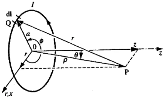
Fig. 3.1 Current Loop and Coordinate System3

where

PO = 4;r -1 % is the permeability of free space I - is the total current flowing in the conductor

di - is the vector whose magnitude is the length of infinitesimal current carrying segment and whose direction is that of the current

r - is the vector from the field point to the infinitesimal conductor element

For a circular loop of wire of radius a carrying current I , a small segment dl produces magnetic field of magnitude

dB = 'o I -dl

dB=-- + 2

.(3.3)

4)r z2 +a'

The direction of this magnetic field is perpendicular to the line connecting dl and the point on the axis. The components parallel to the line cancel due to the symmetry of the problem. Integrating the perpendicular components around the circle, we obtain

dl 2 +a2

B = dB = --- =in _ dl

4)r z2+a2 4)r z2+ a2

90 a 21ra= _{aoia2 (3.4)}

(z2+a2 2(z2+a2

We can now proceed to compute the derivatives of this field:

vB

a CB -3a 2

z 2foja2z

aZ

(a2+z2)Y

(a2+z2)X

_B 2a 3a3 poIa (a2 -2z2) (3.6)

5a (a2 + z2 ~(a2 +z2) 2 (a2 +z2)(3

a2B 4az 5az(a2 _-2z2) (3a2 _-2z2)

azaa (a2 + z2)X (a2 + z2) (a2 +Z2)Y (3.7)

a (a 2B (3a2 -2z2) 12az2

2la2 (3a2 -2z2)

aa

aZ2

_{(a2+z2)2 (a2+z2)2}

(a2+z2)Y

(3a4 -24a 2_z2

+8z4)

2

( a 2 + 2 )Y

=~i320Ia (a2+z2)%

3.2 Rotation vs. Translation Revisited

This would be a convenient point to revive the following questions regarding the relative time scale for rotational and translational motions of a magnetic dipole:

" What is the critical length in this problem, as defined in Eqn. 2.18 ? * How should we modify our analysis from section 2.3 ?

* For a coil of given radius, where on its axis is the difference between rotational and translational dynamics most pronounced ?

The answer to the first question is,

D=VB = . (3.9)

F az I 31z

Computing the spatial derivative and setting it to zero:

aD I a2 +Z2 Z2 a2

-= sgnz-(2- =0, (3.10)

az 3 Z2 3Z2

we discover that D assumes one extremum value at z = a. Since

a2D 2a2 2a2

-~- sgnz---= _{1 3} >0 Vz, (3.11)

az2 3z-1 31

it is a global minimum. Therefore,

2a2 ₂ D 2---=-a. (3.12) 3a 3 and / 3

1

y-cot .- = cot(P. (3.13) 6 2a 4a

Once again, assuming that <-, we obtain that the rotation is at least an order of

a 10

magnitude faster than translation for all angles

(PE

r ,

, (3.14)

110 10 _

which applies to a smaller part of the circle than Eqn. 2.21, but also makes a stronger statement. In either case, the qualitative result is the same: unless the magnet is aligned fairly closely with the field (parallel or anti-parallel), rotation will dominate translation. The above analysis shows that in the worst case scenario, z = a, the angular sector where

3.3 Coil Size Optimization

Based on the expressions for the field and its derivatives, we can now evaluate where on the axis, the coil is most effective in creating a field or field gradient that would control the dynamics of a dipole placed at that location, via equations 2.7 and 2.10. In order to generalize our results for coils of arbitrary radii, we begin by expressing the field and its derivatives in terms of the dimensionless scaling factor, = z / a.

B(, a)1= (3.15) 2 a ( +1 )X VB( ,a)

11=

(3.16) 2 a2(2 +1)Y2 B,(t a) =p1 ) (3.17) a2 ( 2 +1)2 Baz(,a) = -3p01 2 (3.18)

a

3 ₍ 2 _+i)

(3

-24 2+8g4) -[B

(4,a)]=

Poi (324+ I) (3.19) aa _a4(2+1)

The expressions above show that for a given scaling factor,

4,

the magnitude of the axial field varies inversely with the coil radius; that is, when viewed on the same scale, smaller coils produce larger fields. This fact is somewhat bewildering because one's intuition would suggest that the physics remains the same when the coils are scaled the same way. The phenomenon can be explained as follows. A field in space exists due to the motion of charged particles, e.g. electrons inside a circular wire. The current in the wire is

proportional to the linear velocity of the electrons passing through its cross-section at any given time. However, to an observer sitting at the point where the field is measured, the current appears proportional to the number of electrons passing through the cross-section in unit time; hence - to the angular velocity of the electrons. When linear velocity is fixed, the angular velocity is inversely proportional to the radius of the wire, and so is the field magnitude. For the same reason, the n,, order derivatives of the field vary as 1 n+1.

The above result suggests that for a fixed ratio of the distance from a coil to its radius, smaller coils are more effective at producing magnetic fields and gradients. However, if we let the ratio change and measure the distance uniformly, it becomes apparent that the field of smaller coils also dies out faster. Thus, there is a tradeoff between efficiency in generating a field and its absolute size, and for a given distance from the center of the coil there exists the optimal coil radii for producing the maximum field and its gradient at that point. We proceed to calculate these radii by setting the appropriate derivatives to zero. In all of the following cases the derivatives are taken with respect to the actual variables a and z even though the results are expressed in terms of the dimensionless

factor

4.

By setting Ba =0, we observe that for a given distance z between a coil center and a point on its axis, the coil that has the radius

creates the largest field per unit current. Likewise, setting B,, = Bza = 0,

similar result for the magnitude of the field gradient:

a A argmaxa{I B,(z, a)

}=

-z = 0.8z =z.

Finally, the optimal

we obtain a

(3.21)

coil size for changing the field gradient is found from - = 0: aa

8x2 _{-24x+3=0 - x 12± 4.3 =1.2,03}

2 -8

a A g=120z _{= Z .}

aV = argmaX

{j Bzz(z,a)I1

_{Y21z=Z,)z (3.22)}

3.4 Off-axis Magnetic Field

4

The exact analytical expression for the off-axis magnetic field of a circular winding can be derived from the magnetic vector potential, expressed in spherical coordinates as

Atp4 dl p Ia 2z2 d A,(p,)=- -I - _{_cos}, 4z r 4r Ip2 +2 0 1-co (3.23) where e= 2apsin9/(p2 + a2 ),

and the rest of the elements are as defined in the figure below. For p >>a (near-field),

p>> a (far-field), or sin9 0 1 (near the axis), e is small and the potential can be approximated as

AO = uIa2 p sin9 (3.24) 4 (p2+a22Y2

The spherical components of the magnetic field B = V x A are then simplified to

B (p,9) = 1 a (sin 9A,) puIa2 cos9

psin9 _a9

2(p2 +a2 )

(3.25)

1

(pA,)

pIa2 (2a2 _p2)sin 0

Boq(p,0)=- 5

p ap 4(p2+a2)Y2

Having obtained an approximate analytical expression for the field, we proceed to compute the exact field components, based on another analytical formula. From the symmetry of the problem, the toroidal and poloidal components of the magnetic vector potential are zero.5 Converting the azimuthal component to cylindrical coordinates

z=psin9, r=pcos9

and introducing the parameter

k2 (z,r)= 4ar (3.26)

(a+r) +z2

we obtain

A, (z, r)= 1 I K -E ,(3.27) )rk r ( 2)

where K and E are the complete elliptic integrals of the first and second kind, defined as

5 From Ampere's law, V x H =

j

and the potential is defined via H = V x A, where

j

is the current that generates the field H which is related to the flux density via B = uH. Because the current is contained in a plane, the potential is perpendicular to the plane and thus contains only azimuthal component.

ir/2 2 K(k)= (I-k'sin2 -,2dx 0 z12 2 2X)Y 2 0

Magnetic field components are then obtained by differentiation:

+ 2 2

(a-r)

2+ -2

-K+ a2 +2 E

(a-r)

+Z 2 2 -Y

These formulas apply both to 2-D and 3-D problems because B has only two components Ar = Az =0 --+ B, =0

and dependence on 9 is removed by rotational symmetry: B(z,r,O) = B(z,r) VO. values for the elliptic integrals are tabulated and easily obtainable on a computer.

The For that reason, equations 3.26 - 3.29 will form the basis for an exact numerical (MATLAB) simulation, which we will introduce in the next chapter.

(3.28) Bz(z~r)= I ~A) = l(a - + r ar 2)L B,.(z, r)=-= --- [(a+ r) az 2yr r r)2+z2]r K (3.29)

tZ

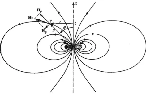
Hp

P r -Z

66

He P

Fig. 3.2 Magnetic Field of a Current Loop'

3.5 The Field of a Thick Solenoid

This section is intended as a brief reference to the simulation software used for field computations. Our purpose here is to demonstrate how the fields were produced and to comment briefly on the results. The code that we chose for our computation is SOLDESIGN. It is a general purpose program for calculating and plotting magnetic fields and Lorentz forces for a system of coaxial, uniform current density solenoids. It was designed and tested at the Plasma Fusion Center at MIT. There are several versions available both for the VAX cluster system and for PC. We used the PC version, which is simplified via reduced dimensions and a lack of graphics, but is nevertheless perfectly adequate for our purposes.

Both the input and output to the program are passed in files of a certain format. The input consists of a sequence of commands that prescribe the geometry of a solenoidal coil and either the overall current density or the total ampere-turns of current flowing through it. When viewed in cross-section, the coil is represented by two rectangles of equal sizes and at equal distances from the origin. (i.e., the center of the solenoid) The geometry is defined by specifying the coordinates of the lower left corner of the left rectangle, its thickness in the x- and y- directions (the radial and axial builds), and a symmetry parameter that allows to include certain reflections of the coils. (e.g., a split pair) The output consists of the coordinates of the field points (the spatial grid), the flux, and the components of the magnetic flux density. A Gaussian quadrature algorithm is employed to integrate the flux and flux density components azimuthally around the perimeter of the coil. Additional details can be obtained from the SOLDESIGN User's Manual available at the Plasma Fusion Center at MIT.

In our setup, the coil is a solenoid of radius 60cm (the average of the inner and outer radii) with square cross-section of 8 cm on the sides and a total current of 500kA-turns flowing through it. The field is computed on a rectangular grid of 61x61 points with the corners at (-31,6), (29,6), (-31,79), and (29,79) cm measured away from the center of the coil. The overall arrangement contains four such coils positioned along the sides of an 80cm square. Because our goal is to analyze the performance of a multi-coil system, we are considering only those regions of space where more than one coil can make a significant contribution to the total magnetic field, given the maximum allowable current levels. Therefore, the operating region does not include 6cm strips adjacent to each of

the coils, because inside these strips, the closest coil dominates all others and the problem of controlling the fields effectively reduces to one dimension. For the multidimensional problem that we are considering, the fields of all the coils are superposed and scaled by their respective current levels. In a later section, we will define how the field values computed for one coil are weighted, rotated, and superposed to produce the fields in a multi-coil arrangement.

3.6 Analytical Approximation

The finite element code presented above produces the most accurate result of all the other methods considered. However, it's disadvantage is that the field values are computed on a discrete spatial grid and a continuous interpolation scheme is required to calculate the fields at all other points in the operating region. There are many general numerical techniques available for that purpose, but it behooves us to attempt a specialized approach by approximating the field on the entire spatial grid by a single analytical function with relatively few parameters. Some precision is necessarily compromised in the process, but the benefits outweigh the losses. First, the computation time is shortened dramatically due to the significant reduction in the complexity of the problem. Second, the resultant expression is simple enough to facilitate analytical approaches to the dynamical analysis and control strategies. In particular, the state-space system of equations can then be expressed and analyzed in a functional form.

There is no reason to expect that dynamical behavior of the system will actually conform to a certain known elementary function; in the most general case, we will merely have a

table of values. A standard approach in such situation would be to approximate the table with a series or an integral of some simple and well-behaved basis functions. However, there is no guarantee on the rate of convergence of these sums, even if the data is reasonably orderly. Furthermore, such representation will not likely be sufficiently intuitive to contribute to the qualitative description of the system. The approach that we have chosen is designed to reflect the qualitative features of our system. For that reason, it is less systematic and, potentially, less precise than a quantitative method. However, we will demonstrate with our approach that considerable numerical accuracy can be achieved without significant increase in the complexity of the model.

3.6.1 The Radial Field Component

The output of the SOLDESIGN is shown in the figure below. The mesh is made crude for enhanced visibility of the individual waveforms. The field is shown in Tesla.

1.5 - --- 0.5 --1.5 _-02 0.8 0.7 0.6 0.5 04 0'' '. _{-. -. ada.2 slc} met ARaial displacement, m

Fig. 3.3 Radial Field component

The shape of the mesh lines suggests that the field is exponentially decaying in the axial (y-) direction and follows an odd-power polynomial in the radial (x-) direction. Focusing on the particular mesh lines, we observe that the exponential curve also has a peak and

appears to consist both of the decay function and of its derivative. This type of behavior is characteristic of the critically damped systems, that have time evolution

f

(t) = p, (t) -e-'I'. For simplicity, we will limit our consideration to the first- and second-order polynomials.

B(x, y) = po (x)e~'l'* + pi (x)ye~'l'' +p,2(x)y2e-,. (3.30)

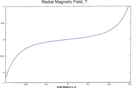
Alternatively, we can first look at the polynomials in x. A typical profile is presented in the figure 1.3. The function appears anti-symmetric around the B-axis and its slope near the origin is sufficiently non-flat to suggest a low degree polynomial, like 3rd or 5th order.

Radial Magnetic Field Component Along the Coil Axis 1.5- 0.5-0 - -0.5- -1-0 0.1 0.2 0.3 0.4 0.5 0.6 0.7 0.8 y, cm

Fig. 3.4 Radial Field Profiles

Because polynomials are easier to approximate than the product of polynomials and exponentials, we have chosen to model the field as

B,(xy) = co(y)x5 _+c

1(y)x' +c2(y)x (3.31)

Therefore, for each value of y = y* we approximate Bx (x, y*) by a polynomial of the 5 h

degree in the odd powers of x. The algorithm to retrieve coefficients {cO,c1,c2

}

is

MATLAB's non-linear best fit, nlinfit, based on Newton's method. It is convenient to - - -- ____

-use when the functional form of the approximation is well known and is neither a pure polynomial nor an invertible function of one. (such as eP(x)

Radial Magnetic Field, T

0.5

-0.5

-

-1--0.2 -0.1 0 0.1 0 .2 0.3

Axid Istaice x, m

Fig. 3.5 Radial Magnetic Field (Radial Slice)

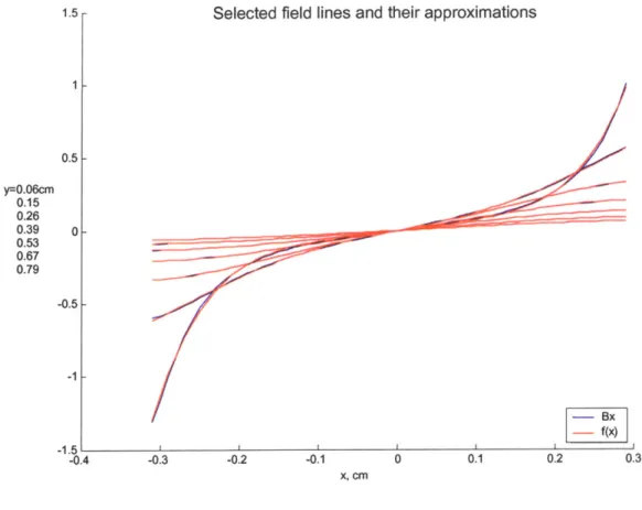
The function nlinfit requires four inputs: the values of the independent and dependent variables; the functional expression relating the two, with unknown but adjustable coefficients; and the initial values of the coefficients. The nature of the method is such that its performance depends substantially on the quality of the initial guess of these coefficients. Therefore, we have adopted an iterative/recursive scheme where the coefficients are first iterated through a crude list of plausible values and the most accurate representation is chosen. Then, starting with the corresponding initial values, the program is run recursively, where the answer from the previous iteration is taken as the input to the next one. The entire procedure is then repeated for each value of y, so that the coefficients are themselves functions of y, as shown in Eqn. 3.31 and in Fig. 3.6,7.

Selected field lines and their approximations 1 - 0.5-y=0.06cm 0.15 0.26 0.39 0-0.53 0.67 0.79 -0.5 -1 --- Bx) -f(x) -0.4 -0.3 -0.2 -0.1 0 0.1 0.2 0.3 X, CM

Fig. 3.6 Radial Field Approximations

As expected from the above analysis, the coefficient curves resemble impulse response of a critically damped system - that is they appear like a product of exponential and polynomial functions of variable y. The fitting is done the same way as for x, with the exception that a different functional relationship is chosen to estimate the coefficients.

co and c2 are estimated with

f(y)

= ae-'+ aiye-kIY, while cl is estimated with

g(y) = boe~"'*+ bye-"' + b2y2eM2y. In total, B, (x, y) is represented with 14 numbers

and has the form:

B,(x, y) = [aO e~kO*y + aolye-k* ] + a10e-oY + a,ye-kiy + a12y 2

e-kl2y 3 +[a20ek2oy + a2ye-ksl 1 ]

where the coefficients are:

a00 ₀₁ a 10 aI 1 2 a20 a21 k k01 k10 k11 k12 k k

-1.53e4 2e3 -433 1451 -99.4 12.42 0.26 14 15 7.7 13.5 14.9 5.04 1.23

Table 1: Radial Field Coefficients

500 400 300 200- I cO 0 0.5 1 y, cm 20 15 10 5 0 -5 c1 0 0 .5 y, cm c2 1.2 1.1 1- 0.9- 0.8- 0.7- 0.6- 0.5- 0.4- 0.3-0.2' 0 0.5 1 y, cm

Fig. 3.7 Radial Field Coefficients

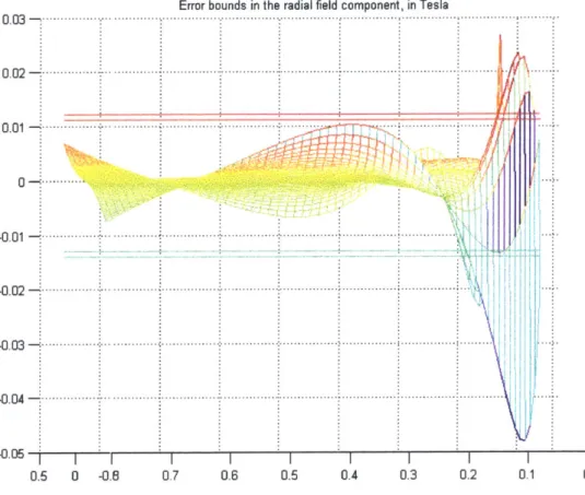
The resulting error in the radial field is computed as e, = Bx (x, y) -,fi (x, y), where the

second term represents the SOLDESIGN field and the first represents its approximation. 10(

-100

It is apparent that the error can be bounded to within 10% of its maximum value for most of the operating region and for y > 20cm it can be further contained by a factor of two. This result is very promising, considering that we are replacing 612 = 3721 numbers with mere 14. With the knowledge of error bounds, we can design robust controllers that are capable of operating with imprecise but bounded measurements of the field. In reality, if the error in the real measurements does not exceed these 10%, the controllers would accommodate both the error in modeling and the errors in the sensor readings.

Error bounds in the radial field component, in Tesla

0 .0 3 , ---. ... - .. --. .-. . .. -. -. _-.-- .... _-- ..._--.- -.--.- ....-. .. ...- .. 0 .0 2 -- --. -. .. --..- -.--.-.--..-.--.-- - -.-.- 0---0 .0 1 - - - --- -- - - -- -.-..-.-.--- --. -0 .02 - -- -- - - --.-.-.-.-. ..--003- - -- -- - - --- --0 .0 4 -. .... ...- .-- -- ... --.. -.- ... .. . -.-.-. -0. 05 0.5 0 -0.6 0.7 0.6 0.5 0.4 0.3 0.2 0.1 0

3.6.2 The Axial Field Component

The approach is the same as for the radial component. First, the shape of the field is determined both in the radial and in the axial cross-sections. Then, the simpler of the two representations is considered and its coefficients are computed as a function of the other variable. Then, similar fitting is performed for each of the coefficients.

The axial field is represented as a mesh in Fig. 3.9. Axial Field Component, T

1.2 ---

----0 - - - - - ~- -

----0.4 --

-1.2 0

-0.4 0.8 0.7 0.6

radial distance (x), m axial distance (y), m

Fig. 3.9 Axial Field Component

Just like the radial field component, the axial one falls off exponentially in the axial direction. However, unlike the radial component, it follows an even-powered polynomial

in the radial direction. Approximating the field in the axial direction with the sum of products of exponential and polynomial functions, we obtain

B,(x,y) = ao(x)ye* (x)y + a,(x)e-kl(xY (3.32)

The coefficients are then fitted with a polynomial in the even powers of x. As shown in Fig. 3.10, the results are not very promising because the coefficients vary sporadically and cannot be easily approximated with polynomials. Some of them (aO and a, ) actually vary exponentially in the steep regions and polynomially in the valley around the origin.

.4 -0.2 0 0.2 0. X, Cm -0.2 0 X, Cm 4 2 0 -2 kO -0.4 -0.2 0 0.2 0. X, Cm 10 4 0.2 0.4 15 10 5 -0.4 -0.2 0 X, Cm 0.2 0.4

Fig. 3.10 Axial Field Coefficients (axial)

Alternatively, we can first approximate the axial field in the radial direction and then fit the coefficients along the y-axis. As evidenced in Fig. 3.11, the functions of x are all

aO 4-3 2 1 --0 a al 4 2.5 2 1.5 1--0.4 k1 - -- - -- --

---even and B, can be approximated directly as a polynomial in x2_{. Furthermore, we can try}

to normalize either x or x2 _{by their variances to obtain a better fit with fewer coefficients.}

The procedure for polynomial approximation is more straightforward than nlinfit. First, the Vandermonde matrix V is formed, whose elements are the powers of

=

x2_.

V =4,"~, (3.33) where n is the largest power of

4

and thus 2n is the largest power of x. Then, the coefficient vector, p, is a solution to the least-squares problem:

p = V-1 -y =(Q -R)' -y =R-1 -Q-1 -y =R 1 .QT _{.y, (3.34)}

where y is the vector of data points and QR-factorization (Cholesky) decomposes V into an orthonormal matrix Q and an upper-triangular matrix R. It is, essentially, an instance of the Gram-Schmidt orthogonalization, where

T T T .

1

qv, q, v2 q1, v3 :

V =v, v2 v3'' j=q q1 2 3 2v 2 qv 3 - QR, (3.35) q3 V3

and the columns of Q are chosen so that q, is in the direction of v1, q2 is in the plane of

v, and v2, etc. The key is to make R invertible, which will happen whenever the number

of data points is greater than the degree of the polynomial and whenever the data points are not repeated. Normalizing the data can also effect the conditioning of R and so, we will consider the polynomials in

/2 _ 222 _

{=x 2

a X and A=x2 x

std(x2_{)I var(x)}

The data is not centered because the coefficient functions are already symmetrical around the origin. The least-square procedure thus projects, one by one, the powers of x onto the data, so that at each step, the approximation error is orthogonal to all the powers considered.

The first five terms in the polynomial expansion were sufficient to approximate the field to within several percents of its nominal value. The coefficient functions are displayed for three different representations of data in Fig. 3.12. Certain complications arise when the data is not normalized. For example, there is a large spread in the coefficient values even though, as verified experimentally, all five coefficients are needed to achieve a reasonable fit. The first representation is thus discounted and the other two are compared. As expected, they appear fairly similar in coefficient values, although the waveforms in the third representation are slightly more amiable to approximation. Therefore, the third approximation is chosen and curve fitting is performed with nlinfit using exponential-polynomial functions of the type considered above. (Eqn. 3.32)