James B. Orlin* July 1982
Working Paper #1331-82
* Work supported in part under ECS-8205022, National Science Foundation, entitled "Research Initiation: Dynamic/Periodic Optimization Models".
This paper presents and solves in polynomial time the dynamic
matching problem, an integer programming problem which involves matchings in a time expanded infinite network. The initial model is a finite directed graph G = (V,E) in which each edge has an associated real-valued weight and an integral distance. We wish to "match" vertices over an infinite horizon, and we permit vertex i in period p to be matched to vertex j in period r if and only if there is an edge e = (i,j) of E with distance r-p or else an edge e = (j,i) of E with distance p-r. Equiva-lently, we construct a "dynamic graph" in which there is an edge incident to vertex i-p and to vertex j-r in the above cases. The weight of this matched edge in the dynamic (time expanded) graph is the weight of e.
The dynamic matching problem is to determine a matching M in the
dynamic graph such that M has a maximum long run average weight per period. We show that the infinite horizon dynamic matching problem is linearly transformable to the finite horizon Q-matching problem, which is shown to be solvable in polynomial time in Part II of this paper.
I. Introduction
In this paper we consider the dynamic matching problem, a matching problem defined on infinite dynamic (periodic, time-expanded) graphs in
which the objective is to maximize the average weight per period of a (periodic) matching. We show that the infinite-horizon dynamic matching problem is
linearly transformable to the finite horizon quasi-dynamic fractional matching problem, which is shown to be solvable by a polynomial time algo-rithm in Part II of this paper.
One can pose other problems on dynamic graphs such as network flow problems, connectivity problems, independence set problems, etc. Orlin (1981a and b) has shown that the dynamic network flow problem is poly-nomially solvable, whereas the hamiltonian path problem, the maximum inde-pendent set problem, the 3-colorability problem and others are all
P-Space hard. (See Garey and Johnson [1979] for definitions). Thus the polynomial solvability of the dynamic matching problem highlights the difference between polynomially-solvable graph problems and NP-hard graph problems as generalized to dynamic graphs.
2. Finite Graphs and Dynamic Graphs
Let G = (V(G), E(G)) be a finite directed graph such that
V(G) = {l,...,n, and each edge e E(G) has an associated distance d(e) an an associated weight w(e). The distance d(e) may be interpreted as
the number of periods separating the head of e from the tail of e. From G we form an infinite undirected graph G = (V(G) , E(G-)), where
V(G-) = {v: v V(G) and p Z, th
and v is called the p copy of vertex v. (Here Z denotes the set of integers.) Moreover, each edge e(u,v) E(G) induces an infinite set of edges (u , v d(e):p Z}each with weight w(e), and (up vp+d(e)) is the pth copy of edge e. The set E(G°) consists of all copies of all edges of E(G). Any infinite graph that is isomorphic to GCO for some finite graph G
is called a dynamic (or time expanded) graph. In Figure 2.1 b, we illustrate a dynamic graph, which is induced from the graph in Figure 2.la.
Ford and Fulkerson [1958] used (finite horizon) time-expanded networks in order to model dynamic flows evolving over a fixed number of periods. Subsequently a number of authors have investigated dynamic network flows
(either finite or infinite horizon) including Gale [1959], Minieka [1973], Orlin 1981a], Halpern [1979], Jarvis and Ratliff [1981], White [1972], and Wilkinson [1971] and [1973]. The author [1981a and b] has analyzed other graph theoretic problems on the infinite dynamic networks described above, and has shown that a number of NP-hard problems on finite graphs become P-space hard when generalized to dynamic graphs. (See Garey and
Johnson 1979] for the definitions with respect to P-space hardness.)
Dynamic Matchings
A matching is a set of edges no two of which are incident with a common vertex. We will refer to a matching in a dynamic graph as a
dynamic matching. Suppose M is a dynamic matching. For each integer p, let
w0) = i w(e)
e=(u , v )M and -p < r,s < p
Thus wP(M) is the sum of the weights of all edges in M whose endpoints are in the set {vr:vcV(G), -p < r < p}. A dynamic matching M is called average weight optimal if for all other dynamic matchings M' we have
lim inf p-l(w(M) - wp (M')) > 0.
The dynamic matching problem is to determine a dynamic matching that is average weight optimal.
A dynamic matching is called periodic with period t if the following is true: the pth copy of edge eE(G) is in M if and only if the (p+t)th copy of edge e is in M for all eE(G) and peZ. The following elementary result is a specialization of a result proved in Orlin [1981b].
Remark 1. For each instance of the dynamic matching problem, there is an optimal average weight matching that is periodic.
Henceforth, we restrict attention only to those dynamic matchings that are periodic. Unfortunately, the periodicity of the matching does not in and of itself lead to an efficient algorithm because the period length is not, in general, polynomial in the problem size. Nevertheless, since we may place an a priori finite upper bound on the period length, and since the dynamic matching problem reduces to an ordinary matching problem if the period length is fixed, we may solve the dynamic matching problem as a finite sequence of matching problems.
As is well known, Edmonds [1965a and b] was the first to provide a polynomial time algorithm for the non-bipartite matching problem. Since that time, many authors including Cunningham and Marsh [1978], Even and Kariv [1975], Gabow [1976] and Lawler [1976] have provided increasingly more efficient algorithms for various types of matching algorithms.
Figure 2.la A 1-period digraph with associated edge distances. 1 ... 2 ... 3 ... 4 ... 5 ... p p+l p+2 p+3 p+5 p+6
Figure 2.lb The dynamic graph
of Figure 2.la.
3. Quasi-Dynamic Fractional Matchings
Our method for solving the dynamic matching problem is as follows. First we define _ quasi-dynamic fractional matching problem, a finite graph theoretic problem that is closely related to the dynamic matching
problem. We then show that a quasi-dynamic fractional matching of weight W "induces" a dynamic matching whose average weight per period is W/2. Finally, we
use the quasi-dynamic fractional matching duality theory proved in Part II of this paper in order to prove that a maximum weight quasi-dynamic fractional matching induces a dynamic matching of maximum average weight per period.
Graph Theoretical Preliminaries
Below we introduce some graph theoretic definitions and notation most of which is common to the literature although not universal. A
path in a directed graph G is a sequence P = v elvl... ekvk such that V(P) = {v0,...,vk} is a subset of V(G) (although we do not assume
that the vertices of P are distinct); E(P) = {el,...,ek} is a subset of E(G); for 1 < j < k, either vj_1 is the tail of ej and v is the head of e. or else v. is the tail and vj_ is the head; in the former case
J J J-l
e. is called a forward edge of p; in the latter case e. is called a backward edge. The path P is simple if V(P)I = k+l. The weight of a
path P is the sum of the weights of the edges of E(P), and we denote it as w(P). The distance of a path P is the sum of the distances of the forward edges of P minus the sum of the distances of the backward edges of P and we denote the distance of P as d(P). The path P is a circuit if
JV(P) = k, v0 = Vk, and k > 1. A circuit C is called trivial if it is a
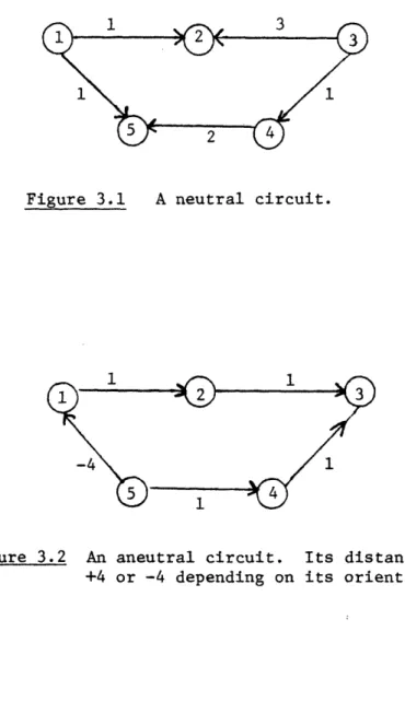
2-edge circuit in which the same edge appears twice. A circuit C is called neutral if d(C) = 0, and it is called aneutral if d(C) 0. Figures 3.1 and 3.2 display a neutral and an aneutral circuit respectively.
Figure 3.1 A neutral circuit.
Figure 3.2 An aneutral circuit. Its distance is +4 or -4 depending on its orientation.
For each set ScV(G), we let G( CS) denote the set of edges having exactly one endpoint in S, and we let yG(S) denote the set of edges having both endpoints in S. (Henceforth, in cases in which there is no ambiguity we will drop the subscript G from 6 and y). We will let (v) (resp., y(v)) denote the set ({v}) (resp., y({v})). Thus y(v) is the set of loops in E(G) both of whose endpoints are vertex v.
A fractional matching is a collection X of vertex disjoint circuits such that each circuit in X is either trivial (2 edges) or else is odd, The weight of a fractional matching is the sum of the weights of the circuits in C. (Fractional matchings are often referred to as
2-matchings, for example in Cornuejols and Pulleyblank [1980].)
A quasi-dynamic fractional matching is a fractional matching with the additional property that all of the odd circuits in the collection
are aneutral. (Of course, all of the trivial circuits are by definition neutral.) Henceforth we will refer to a quasi-dynamic fractional matching by the
abbreviated name Q-matching. We will often denote a Q-matching as an ordered pair (M,Q) where M is the subset of edges of E(G) corresponding to the trivial circuits of the Q-matching and Q is a collection of odd aneutral circuits. A Q-matching (M,Q) is portrayed in Figure 3.3. The set M = {(6,4)} and Q contains the two odd aneutral circuits in boldface.
A subgraph H of G is said to be rooted if there is a designated vertex VH of H that is the root. A subgraph H of G is said to be odd (resp., even) if IV(H)I is odd (resp., even).
The close relation of Q-matchings to dynamic matchings is a consequence of the following lemma proved by the author (1981a).
Lemma 1. Let G = (V(G),E(G)) be a finite directed graph with edge distances d = (d(e)), and let G = (V(G ),E(G )) be the induced dynamic
---graph. If C is a cycle in G of distance d(C) = s 0, then the infinite number of copies of the edges of C comprise sl vertex disjoint infinite paths in G.
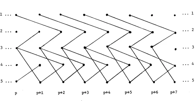
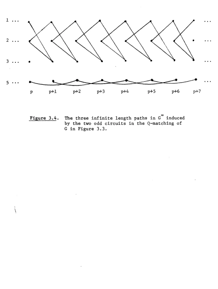
The above Lemma is illustrated in Figures 3.4, the dynamic graph induced by the subgraph G{1,2,3,5}] of G as restricted to vertices 1,2,3 and 5.
Corollary 1. Let G be a finite directed graph, and let G be the induced dynamic graph. Then any Q-matching (M,Q) of G induces a dynamic matching M* of G consisting of all copies of edges e for which e E(M) together with every other edge of the vertex disjoint infinite paths induced by
the odd circuits of Q. Moreover, the weight of (M,Q) is twice the average weight per period of M*.
Proof. The proof is direct and is left to the reader.
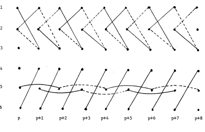
Corollary 1 is illustrated in Figure 3.5 and is the dynamic matching induced by the Q-matching of Figure 3.3.
2
Figure 3.3. A Q-matching with one matched edge and two matched odd aneutral circuits.
2 ...
3 ...
p p+l p+2 p+3 p+4 p+5 p+6 p+7
Figure 3.4. The three infinite length paths in G induced by the two odd circuits in the Q-matching of G in Figure 3.3.
I
1 2 3 4 6 p p+l p+2 p+3 p+4 p+5 p+6 p+7 p+8
Figure 3.5. A dynamic matching induced by the Q-matching of Figure 3.3. (The copies of vertices 7 and 8 are not portrayed since they are unmatched in the Q-matching).
4. Maximum Weight Q-Matchings Induce Average Weight Optimal Dynamic Matchings We have just seen that a maximum weight Q-matching (M,Q) induces a
dynamic matching whose average weight per period is one-half of the weight of (M,Q). In this section we show that the induced dynamic matching is indeed average weight optimal. The proof technique relies on some
elemen-tary properties of dynamic integer programs described below.
Dynamic Integer Programs
The dynamic integer programming problem consists of all instances of (4.1)
Maximize lim inf (2t+l)-1 wx (4.la)
t -+ p=-t
Op +
~~~
-i- Ap+q q . b for all p E Z (4.lb) Subject to A x P + ... + AqxP+q bxp > 0 integer for all P e Z (4.1c)
where A ,...,Aq are m x n integer valued matrices, w and b are vectors, and xP is the vector of decision variables for period p.
We note that the dynamic matching problem is the special case of the dynamic integer programming problem in which b is a vector of all l's and each column of the 2-way infinite constraint matrix is a 0-1 vector with exactly two l's.
The dynamic linear programming problem is the problem obtained from the dynamic integer programming problem by relaxing the integrality con-straints. A sequence x = (x P ) of decision vectors is said to be stationary
P P+l
if x = x for all p Z. The author [1981a] proved that if there is an optimum average-weight sequence x = (x) for a dynamic linear programming
problem, then there is such a sequence that is stationary. Here we state and prove a weaker result (which is strong enough for our purposes),
-15-Lemma 2. Let x = (xP) be an optimal periodic solution for a dynamic integer programming problem. Then there is a stationary continuous solution y that is fe, - ble for the continuous relaxation and whose average weight per period is at least as great as that of x.
P - l x
Proof. Suppose x is periodic with period t. Le y = t (x +...xt) for all pZ. It is easily verified that y is a stationary solution that is feasible for the continuous relaxation. Moreover, the average weight per period of y is equal to the average weight per period of x.
Neutral Subgraph
In the case of finite matching problems, Edmonds [1965b] defined a poly-hedral set of constraints that he showed to be the convex hull of the
matching polyhedron. Unfortunately, the convex hull of the dynamic matching polyhedron cannot be expressed as a dynamic linear program.
(The set of facets contains the odd set constraints defined by Edmonds
[1965b], and there are a countably infinite number of finite odd sets containing any specified edge of E(G ). Thus any dynamic linear programming
formu-lation would involve infinite matrices A,...,A , which is forbidden.) Nevertheless, we can solve the dynamic matching problem through a minor modification of Edmonds technique. It suffices to add a subset of poly-hedral facets to the dynamic integer programming formulation of the dynamic matching problem with the property that the resulting linear relaxation is "optimally solved by a Q-matching." Then by Lemmasl and 2, the induced
dynamic matching is average weight optimal. The subset of polyhedral facets that we consider may be referred to as "neutral set constraints", as
defined below.
Let H be a subgraph of directed graph G. We say that H is neutral if H contains no aneutral circuit. The following characterization of connected neutral subgraphs is elementary and is stated without proof.
Lemma 3. A connected subgraph H of the digraph G is neutral if and only if for every two vertices u,v £ V(H) it follows that the distance of a path from u to v in H is independent of the path.
Corollary 2. Let H be a rooted connected neutral subgraph of the digraph G. For each vertex v V(H), let dH(v) be the distance of a path in H from the root to v. Then for each edge e = (u,v) E(H) it follows that d(e) = d(v) - d(u).
Let H be a rooted neutral connected subgraph of the digraph G and let d(v) = dH(v) be the distance in H from the root to vertex v. Then the
th
p copy of H is the unique subgraph H of G such that (1) V(H) = {vp+d(v):V C V(H) ,
(2) E(H) = {all copies of E(H) with both endpoints in V(HP)}.
By Lemma 3 and its Corollary, the pth copy of H is well defined and has exactly one copy of each vertex and edge of H. (Note that this latter property would not be true if H has an aneutral circuit.) Therefore, the following result is immediate.
Corollary 3. Let H be an odd rooted connected neutral subgraph of the directed graph G such that V(H)l = 2k+l. Suppose M is a dynamic matching of the dynamic graph G induced from G. Then for each integer p, the number of dges of E(H ) in M is at most k.
The Dynamic Matching Problem with The Neutral Subgraph Facets
We present below a dynamic integer programming formulation of the dynamic matching problem in which we incorporate the implied constraints
Let G = (V(G), E(G)) be a directed graph, and suppose that E = {el,...,e }. Let N be the set of all of the odd connected neutral subgraphs of G (a set
bounded in cardinality by the number of subsets of edges of G). Moreover, let us assume that each neutral subgraph H in N is rooted (for example, at the lowest index vertex of V(H)).
We let x = 1 or 0 accordingly as edge e of V(G®) is or is not in
J 3
the matching. We let wj = w(ej). We then formulate the dynamic matching problem as the dynamic integer program (5.1).
t
Maximize lim inf (2t+l)-1 w.xp (5.la)
t p=-t ej E(G) 3 J
Subject to E x? < 1 for all vV(G) (5.lb) 3
ePe6(vr) and all rZ
3
XP < (1/2)(IV(H)I-1) for all HN (5.1c)
ePeE(H ) and all rZ
3 r
x > 0 integer for all eE(G) (5.1d) 3
-and all rZ .
Theorem 1. Let G be a directed graph and let G be the induced dynamic graph. Then a maximum weight Q-matching for G induces a dynamic matching
co
for G that is average weight maximum.
Proof. Let (M,Q) be a maximum weight Q-matching of G. By Corollary 1, (M,Q) induces a dynamic matching M' of G whose average weight W' per period is half of the weight of (M,Q). Thus it suffices to show that there cannot be a dynamic matching whose average weight per period exceeds W'.
By Lemma 2, it suffices to show that the maximum weight per period of a stationary continuous-valued solution to (5.1) does not exceed W'. We can determine such a maximum average weight stationary solution y = (y.) by observing first that the value of yP is independent of the superscript p,
·-··---·--·-·--·-and then substituting into the dynamic integer program (5.1) to obtain the linear program (5.2).
Maximize wy.j (5.2a)
ej.E(G) J
Subject to y < 1 for all vV(G) (5.2b)
e.6(v)
y. < (1/2)(iV(H)f-1) for all HN (5.2c) ej.E(H)
yj > 0 for all e.cE(G) . (5.2d)
The stationary solution y can be obtained by repeating the solution y in each period, and thus the average weight per period of y is the same as the weight of wy.
We observe that any Q-matching (M,Q) with weight W* induces a solution y = (y ) for (5.2) with wy = (1/2)W* given by
1 if e is an edge of M yj 1/2 if e is an edge of Q
0 otherwise .
The proof will be complete if we demonstrate that (5.2) is optimized at a Q-matching. This final result is Theorem 3 in Part II of this paper, and an algorithmic proof is provided there. O
\We note that the time to solve the dynamic matching problem is thus equal to the time to solve the Q-matching problem. In Part II of this paper we provide an (IV(G)13) time algorithm to solve both problems.
6. Rmarks on The Methodology
The above solution technique for dynamic matchings is an example of an integer program solved via rounding. The dynamic integer programming problem is equivalent to (5.1). The solution technique may be viewed as
rounding an optimal continuous stationary solution. (Each edge e in a J
circuit of Q is such that x? = 1/2 for all p. Half of these variables are rounded up whereas the other half are rounded down.)
The idea of rounding may seem incidental to the solution technique because in a 0-1 integer program any change in a fractional variable may be viewed as rounding. However, the structure of dynamic integer programs suggests that the rounding depends on the basis structure of the linear relaxation (5.2). Moreover, the rounding technique here is quite similar to the one developed by the author [1981a] for the dynamic network flow problem. We conjecture that a similar rounding technique will be successful if we consider b-dynamic matchings, i.e., if we allow the right-hand side of the dynamic matching integer programming problem to be any positive integer vector b.
7. Applications
A number of applications of matchings may be extended quite directly to dynamic matchings if the scheduling process is both dynamic and periodic. Below we provide one such application. Although the example is somewhat
artificial, we hope that it illustrates the modeling of the dynamic/periodic aspect of scheduling.
An Application to Dynamic Pairings of Workers
Consider a firm that wishes to pair its workers on projects on each day over an infinite horizon. The projects may be split so that worker i can complete half of any project and the remaining half may be completed s days later by worker j at a value w to the firm. In this case we have vertices i representing worker i on day p, and there is an edge joining ip to j s with weight w. The objective is to pair workers so as to maximize the per-day value to the firm.
A Potential Application to Dynamic Integer Programming
Not only is dynamic integer programming P-space hard, but most special cases of it are also P-space hard, as proved by the author [1981b]. For instance, the special case of determining whether there is a feasible solution to (7.1) is P-space hard.
i i+l
Ax + Bx = 1 for iZ
(7.1) 0 < xi < 1; xi integer for ieZ
where A and B are m x n matrices of O's and l's such that each column of [A] has at most three l's.
As an example of a dynamic integer programming set cover problem, consider the following periodic single processor scheduling problem which was formulated and communicated to the author by C. L. Liu [1979]. Let
{J' ... J } be a set of n jobs each of which has a unit processing time and must be scheduled "periodically". The objective is to determine an infinite horizca schedule such that exactly one job is processed in every period and such that the maximum number of periods between successive proce of job J. is at most t..
We can formulate the periodic processor scheduling problem as a dynamic integer program as follows:
1 if job J. is processed in period p Let xp 0
1i if otherwise
Then determine a sequence x = (x?) such that n xp = 1 for p = 1,2,3, i=l P+ti-l xi > 1 for p = 1,2.3, .... and
i
= 1, ..., n j=PxPi e {0,1} for all i,p.
A promising application of dynamic matchings may be as subroutines in heuristics for solving dynamic combinatorial optimization problems such as the above processor scheduling problem. In particular, Nemhauser and Weber [1975] showed how to solve the covering problem using a
Lagrangean relaxation in which each subproblem is a matching problem. It is easy to extend their technique so as to transform dynamic set covering problems into dynamic matching problems with side conditions. It is an interesting open question as to whether the resulting Lagrangean relaxation can be exploited so as to provide a more efficient solution technique for the covering problem.
ACKNOWLEDGEMENTS
I wish to thank Professor Arthur F. Veinott for his help during the initial stages of this research. I also wish to thank John VandeVate for his careful reading of the manuscript and for his suggestions that led to improvements in the exposition.
References
Cornuejols, C. and W. Pulleyblank. 1980. A Matching Problem with Side Constraints. Discrete Mathematics 29, 135-159.
Cunningham, W. and A. Marsh III. 1978. A Primal Algorithm for Optimum Matching. Mathematical Programming Study 8, 50-72.
Edmonds, J. 1965a. Paths Trees and Flowers. Canadian Journal of Mathematics 17, 449-467.
Edmonds, J. 1965b. Maximum Matching and a Polyhedron of (0,1) Vertices. Journal of Research of the National Bureau of Standards. 6913, 125-130. Even, S. and Q. Kariv. 1975. tn 0(n 5/2) Algorithm for Maximum Matching
in General Graphs. In 16 Annual Symposium on the Found. of Comp. Science, IEEE, New York, 100-112.
Ford, L. R. and D. R. Fulkerson. 1958. Constructing Maximal Dynamic Flows from Static Flows. Operations Research 6, 419-433.
Gabow, H. 1976. An Efficient Implementation of Edmonds' Algorithm for Maximum Matchings on Graphs. Journal of the Association of Computing
Machinery, 23, 221-234.
Gale, D. 1959. Transient Flows in Networks. Michigan Math Journal 6, 59-63.
Garey, M. R. and D. S. Johnson. 1979. Computers and Intractibility: A Guide to The Theory of NP-Completeness. W. H. Freeman and Company, San Francisco.
Halpern, J. 1979. A Generalized Dynamic Flow Problem. Networks 9, 133-167.
Jarvis, J. and H. D. Ratliff. 1981. Some Equivalent Objectives for Dynamic Network Flow Problems. Management Science 28, 106-109. Lawler, E. L. 1976. Combinatorial Optimization: Networks and Matroids.
Holt, Rinehart and Winston, New York.
Minieka, E. 1973. Maximal Lexicographic and Dynamic Network Flows. Operations Research 21, 517-527.
Nemhauser, G. and G. Weber. 1979. Optimal Set Partitioning, Matching, and Lagrangian Duality. Naval Research Logistics Quarterly 26, 553-563.
Orlin, J. 1981a. Dynamic Network Flows. Ph.D. dissertation. Department of Operations Research, Stanford University, Stanford, CA.
Orlin, J. 1981b. The Complexity of Dynamic Languages and Dynamic Optimization Problems. 13th Annual Symposium on the Theory of Computing, 218-227.
Orlin, J. 1982. Dynamic Matchings and Quasi-Dynamic Fractional Matchings II.
White, W. 1972. Dynamic Transshipment Network: An Algorithm and its Application to The Distribution of Empty Containers. Networks 2,
211-236.
Wilkenson, W. 1971. An Algorighm for Universal Dynamic Flows in A Network. Operations Research 19, 1602-1612.
Wilkenson, W. 1973. Min/Max Bounds for Dynamic Network Flows. Naval Research Logistics Quarterly 20, 505-516.
I