Publisher’s version / Version de l'éditeur:
International Journal of Lighting Research and Technology, 33, 2, pp. 97-116,
2001-05-01
READ THESE TERMS AND CONDITIONS CAREFULLY BEFORE USING THIS WEBSITE.
https://nrc-publications.canada.ca/eng/copyright
Vous avez des questions? Nous pouvons vous aider. Pour communiquer directement avec un auteur, consultez la première page de la revue dans laquelle son article a été publié afin de trouver ses coordonnées. Si vous n’arrivez pas à les repérer, communiquez avec nous à [email protected].
Questions? Contact the NRC Publications Archive team at
[email protected]. If you wish to email the authors directly, please see the first page of the publication for their contact information.
This publication could be one of several versions: author’s original, accepted manuscript or the publisher’s version. / La version de cette publication peut être l’une des suivantes : la version prépublication de l’auteur, la version acceptée du manuscrit ou la version de l’éditeur.
Access and use of this website and the material on it are subject to the Terms and Conditions set forth at
Lighting quality recommendations for VDT offices: a new method of
derivation
Newsham, G. R.; Veitch, J. A.
https://publications-cnrc.canada.ca/fra/droits
L’accès à ce site Web et l’utilisation de son contenu sont assujettis aux conditions présentées dans le site LISEZ CES CONDITIONS ATTENTIVEMENT AVANT D’UTILISER CE SITE WEB.
NRC Publications Record / Notice d'Archives des publications de CNRC:
https://nrc-publications.canada.ca/eng/view/object/?id=daea75b6-e8df-487c-858c-1e3b91b1e319 https://publications-cnrc.canada.ca/fra/voir/objet/?id=daea75b6-e8df-487c-858c-1e3b91b1e319Newsham, G.R.; Veitch, J.A.
A version of this paper is published in / Une version de ce document se trouve dans : International Journal of Lighting Research and Technology, v. 33, no. 2, 2001 pp.
115-134
www.nrc.ca/irc/ircpubs
Summary An experiment in a mock-up office space gave occupants control over
dimmable lighting circuits after a day working under pseudo-random lighting conditions. Data analysis indicated that the lighting experienced during the day influenced the changes in lighting made at the end of the day. Occupants chose to reduce screen glare if any existed. Even after allowing for the effect of glare, desktop illuminance at day’s end varied with the illuminance experienced during the day. Regression of these end-of-day choices relative to the illuminance experienced during the day can yield a preferred illuminance, equivalent to the daytime illuminance at which no change was preferred at day’s end. Using this method, preferred
illuminances in the range 200 to 500 lx were derived. Preferences for luminance ratio were also derived. Interestingly, the deviation between participants’ lighting
preferences and the lighting they experienced during the day was a significant predictor of participant mood and satisfaction.
Lighting quality recommendations for VDT offices: A new method of derivation
G R Newsham, PhD and J A Veitch, PhD
Institute for Research in Construction, National Research Council Canada, Ottawa, Ontario, K1A 0R6, Canada. E-mail: [email protected]
A version of this paper has been accepted for publication in
List of symbols
LC The participant having control over lighting choices at the start of the day
NC The participant who did not have control over lighting at the start of the day, but who got to express their preference at the end of the day VDTG
% Fraction of VDT screen area – when dark – occupied by visible glare image, > 40 cd/m2 (%)
VDTG
L Mean luminance of visible glare image (cd/m2)
ED Illuminance measured on the desktop, close to the VDT, but on the opposite side from the task light (lx)
LMM Natural logarithm ratio of maximum to minimum luminance in the field of view; luminance values averaged over a target approx. 1° square VDT-LCG
L VDTGL of luminous conditions chosen by the LC participant at the start of the day, and prevailing during the day (cd/m2)
LCE
D ED of luminous conditions chosen by the LC participant at the start of the day, and prevailing during the day (lx)
NC
ED ED of luminous conditions chosen by the NC participant at the end of the day (lx)
LCLMM LMM of luminous conditions chosen by the LC participant at the start of the day, and prevailing during the day
NCLMM LMM of luminous conditions chosen by the NC participant at the end of the day
∆ED NCED minus LCED (lx)
∆LMM NCLMM minus LCLMM
∆VDTG%
VDTG
% of luminous conditions chosen by the NC participant at end of day minus VDTG% of luminous conditions chosen by the LC participant at start of day
∆VDTGL
VDT
GL of luminous conditions chosen by the NC participant at end of day minus VDTGL of luminous conditions chosen by the LC participant at start of day
1. Introduction
Today’s lighting recommendations are based on the consensus and collected wisdom of the technical committees of professional organisations responsible for the
documents. IESNA, for example, provides recommendations through consensus using rigorous procedures and committees made up of diverse representation (1). Nonetheless, the resulting recommendations are not necessarily grounded in the latest empirical research (2). This is one reason for the wide variation in illuminance
recommendations between different countries and over time (3). Consensus-based procedures are a necessary means to reach practical recommendations given incomplete technical information (4), but sound empirical evidence about the effects of lighting on humans is an essential part of the information-gathering process.
Lighting recommendations have emphasised lighting for visibility during much of this century, but recently the concept of lighting quality, about which much less is known (5,6)
, has received increased attention. Lighting quality has been defined as the degree to which a lighting installation fulfils human needs within constraints such as
economics, energy consumption, and maintenance (7,8).
Among the outcomes that have been suggested as targets for recommendations based on lighting quality is individual preference for luminous conditions. Baron, Rea, and Daniels hypothesised that luminous conditions that people prefer will create a state of positive affect (good mood) that will lead to desirable outcomes like improved cognitive task performance, increased pro-social behaviour, and more creative problem-solving (9).
A recent experiment at the Institute for Research in Construction was designed to test the hypothesis that giving individuals control over lighting will lead to improved task performance and better mood and satisfaction. Participants worked in pairs for a full-day session under lighting conditions chosen by one member of the pair at the start of the day. At the end of the day, the second participant chose the lighting conditions that they would have preferred. Extensive data on both participants' lighting choices, and satisfaction, task performance, mood, and visual performance during the working session, were collected. Parts of the data, including detailed protocols and analysis of the principal hypothesis, have been reported elsewhere (10-12).
In addition to the original hypothesis, post-hoc data analysis suggested a novel technique to objectively derive preferred luminous conditions. This paper reports on this novel technique.
2. Methods and procedures
2.1 The experimental space
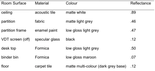
The experiment was performed in a windowless mock-up office space, of 83 m2 floor area. The space contained six workstations, arranged as parallel rows of three along a central spine. Each workstation was designed as a standard North American open-plan arrangement for a mid-level office worker, and measured 6 m2 floor area. Measured room surface reflectances are reported in Table 1.
The lighting system installed in the space was not a typical real-world design, but consisted of groups of differing luminaires intended to broaden the occupants’ choice of luminous environment (the office space layout and lighting system are shown in Figure 1(a)). The luminaires were connected to four independently controllable circuits:
• recessed 1’x 4’ deep-cell parabolic louvered luminaires overhead, 2 x 32W lamps per luminaire (labelled 1 in Figure 1(a));
• recessed 1’x 4’ deep-cell parabolic louvered luminaires (identical to those in the previous bullet) at the perimeter of the space, 2 x 32W lamps per luminaire (labelled 2 in Figure 1(a));
• partition-mounted indirect lighting, 2 x 32W lamps per 4’ luminaire (labelled 3 in Figure 1(a)); and,
• under-shelf task lighting 1 x 17W lamps per 2’ luminaire (labelled 4 in Figure 1(a)).
The first three circuits were continuously dimmable while the task lighting had a simple on/off control. All luminaires used electronic ballasts and 3500K T8 lamps (CRI=80).
2.2 The participants and the experimental procedure
The experiment required a total of 120 temporary office workers. On each day, two participants (matched by age and sex) were seated at the two centre workstations (labelled WS2 and WS5 in Figure 1(a)). Of each pair, one participant (randomly assigned) was designated as the lighting controller (LC), while the other was identified
as having no control (NC). The participants were also randomly assigned to workstations.
At the start of the day LC was shown into the mock-up space which was lit with a standard base-case lighting design featuring the dimmers at their mid-setpoints and the task lighting on. LC was then invited to adjust the lighting system to his/her preference; NC was not in the mock-up space during this part of the procedure. LC adjusted the lighting using a dimmer panel within his/her workstation similar to a common wall-mounted architectural lighting controller. The panel had an up and down arrow for each dimmable circuit. Each circuit also had a vertical set of sixteen LEDs; when the arrows were pressed the number of LED’s lit changed accordingly. Figure 1(b) shows the relationship between the dimmer setting and the relative light output for the recessed parabolic fixtures. The relationship is close to linear up to dimmer setting 12, after which there is little change in light output as the dimmer setting is increased.
Both participants were then seated in their workstations, with LC requested not to mention his/her role in choosing the lighting conditions. Because of the symmetry of the lighting design, NC received the same lighting conditions as LC, but was unaware that LC had selected the conditions. The participants then performed a day of office tasks, with appropriate breaks, during which no adjustments to the lighting were permitted.
At the end of the day, NC was given an opportunity to adjust the lighting according to his/her preferences. The starting point for these adjustments was the same base-case LC had seen at the start of the day. At the same time, and in an adjoining room, LC
was asked on a questionnaire to indicate what changes he/she would have made to the original lighting set-up, given the opportunity.
2.3 Tasks performed by participants
In addition to morning and afternoon visual performance tests, the participants
performed a variety of computer-based tasks designed to simulate modern office work (13). These tasks principally involved typing, proofreading, and creative writing. They
also completed computer-based questionnaires (11,13) at various times of the day to assess their satisfaction with, and impressions of: lighting quality and mood; physical comfort; perceived and desired control over environmental features in general; perceived control during the session; and, lighting preferences in general.
2.4 Photometry
The lit environments chosen by the participants were recorded in detail. Spot
illuminance and luminance were measured at a variety of locations in each workstation and supplemented with digital image analysis of luminance in the field of view. The fraction of each lighting circuit’s maximum output (proportional to the dimmer setting) was also recorded.
The photometric measures of lighting conditions considered in this paper are desktop illuminance, luminance ratio in the field of view, and measures of VDT-screen glare. These are the most common photometric measures used in lighting research and were
highly intercorrelated with other, more complex, photometric measures. Figure 2 details the photometric variables referred to in this paper.
More detail on the experiment method and procedures is provided elsewhere (10-12).
3 Data analysis method
This experiment yielded a very large data set which has been analysed both qualitatively and quantitatively elsewhere (10-12). These prior analyses looked at the effect of choice on satisfaction and performance, the choices made, how these choices compared to existing codes and standards, and the consequences for energy
consumption. Further consideration suggested that these data could be re-analysed to yield objective measures of luminous preference potentially better than simple
measures of central tendency and variability. This method is based on one already familiar to thermal comfort researchers (14).
Consider the NC participants: they were exposed for a six-hour period to pseudo-random lighting conditions (those lighting conditions chosen by the LC participants). The lighting conditions the NC participants chose for themselves at the end of the day – specifically, the deviations from the conditions they were exposed to during the day – can be taken as an measure of their satisfaction with the lighting chosen by their LC partner, or as a measure of their preference for change. The daytime lighting
conditions for which the NC participants, on average, preferred no change may define recommended luminous conditions for VDT spaces. These conditions can be derived by regression of preference for change against the lighting conditions experienced
during the workday. To the authors’ knowledge, lighting data have not been analysed in this way before.
4 Results
For reasons detailed elsewhere (10), 13 pairs of participants were dropped from the data set prior to analysis, leaving a sample size for all analyses of n=47 NC
participants, (21 men and 26 women ranging in age from 18 to 58). Age and sex were previously established as having no effect on lighting choices in this experiment (12).
4.1 Derivation of preferred desktop illuminance
Figure 3 shows a raw plot of ∆ED vs. LCED. The linear regression# is statistically significant (F1,45=29.72, p<0.01), and shows that, given a linear relationship, the desktop illuminance experienced during the day explains 40 % of the variance in the change in illuminance chosen by the NC participants at the end of the day (r2 = 0.40). The regression line crosses the x-axis at 392 lx and has a negative slope: those who experienced high illuminances during the day tended to want lower illuminances, and vice versa.
#
The assumption of a linear relationship between variables is the common starting point in behavioural research, unless there is a strong theoretical reason to assume otherwise. At this point, the goal is to establish relationships between variables, not to calculate the best possible curve fit. We explore other curve fits later in the paper.
However, the post-experiment data indicated that many participants adjusted the lighting (NC), or would have adjusted it if they had had the chance (LC), to reduce glare on the VDT screen from overhead luminaires (10,11). With our lighting design, as with the majority of real-world lighting designs, it was impossible to vary desktop illuminance and VDT glare conditions independently. Therefore, it is likely that end-of-day changes in desktop illuminance are not only a function of desktop illuminance experienced during the day and illuminance preferences, but also occur as a consequence of glare reduction strategies.
To separate these effects graphically a statistical technique called “partialling out” was used. We made the conservative assumption that glare control was the primary cause of end-of-day illuminance changes. Two measures of glare were available, VDTG% and VDT
GL, having been derived in prior work (10). VDTG% has intuitive appeal as a driver of glare reduction strategies, however, ∆VDTGL correlated significantly with a subjective measure of glare (r=-0.31, t=-2.17, p<0.05)∀, whereas ∆VDTG
% did not.Therefore, VDTGL was the glare measure pursued in this analysis*.
The next step is to regress ∆ED vs. ∆VDTGL, and to produce a regression equation. Next take the residual, which is the difference between the actual value of ∆ED and that predicted by the regression equation. The residual is that part of ∆ED not
explained by changes in VDT-screen glare. Finally, the residual of ∆ED was regressed
∀
Note, the significant correlation is negative, as expected: the greater the occupant’s rating of glare during the day, the more they reduced glare image luminance at the end of the day, on average.
* In fact, the analyses reported in this paper were repeated using VDTG
%, but VDTG% proved to be a worse predictor of outcomes than VDTGL.
vs. LCED. This final step generated an equation illustrating how end-of-day desktop illuminance was influenced by illuminance experienced during the day, independent of changes made to affect VDT-screen glare changes. Figure 4 shows the graphs generated by this process.
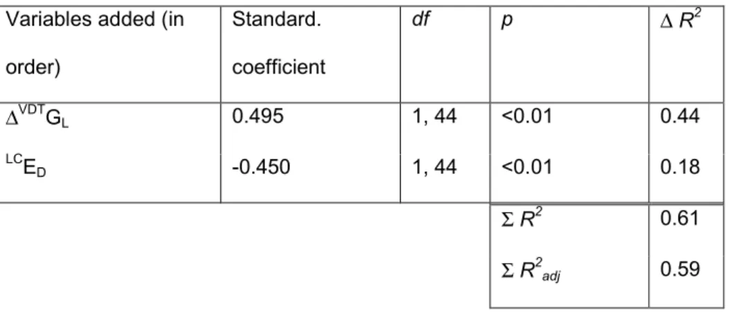
Figure 4(a) shows ∆ED vs. ∆VDTGL. The linear regression is statistically significant (F1,45=34.61, p<0.01, r2=0.44), confirming that, as expected, changing VDT-screen glare conditions has a strong effect on desktop illuminance. The regression line has a positive slope: if glarespot luminance increases so does desktop illuminance. Figure 4(b) shows the residual of ∆ED after the effect of ∆VDTGL is removed vs. LCED. The linear regression is statistically significant (F1,44=19.86, p<0.01, ∆R2=0.18)α, confirming that, even with the effect of glare-driven lighting changes partialled out, end-of-day desktop illuminances still correlate to daytime illuminance experience. Knowing LCED explains 18 % more of the variance in ∆ED than does knowing ∆VDTGL alone, if the relationship is linear. The linear regression line crosses the x-axis at 458 lx and has a negative slope. Therefore, 458 lx could be considered the preferred illuminance for the sample (independent of the effect of glare). It is the illuminance at which, on average, the NC participants would want no change from the conditions they experienced during the day.
α ∆R2
is used here to indicate the additional variance in ∆ED explained by LCED after accounting for the effect of ∆VDTGL. This is calculated using stepwise regression. Step 1: regress ∆ED vs. ∆VDTGL alone (r2=0.44); Step 2: regress ∆ED vs. ∆VDTGL and LC
ED together (R2=0.61), the difference is the variance explained by LCED,=0.18. Similarly, the F-test (F1,44) refers only to that part of the variance in ∆ED due to LCED alone, after the inclusion of ∆VDTGL.
Figure 4(b) also shows the 3rd-order polynomial regression on the same data. The shape of this curve is more appealing theoretically. Rather than specifying a single preferred illuminance, the 3rd-order curve provides a broad plateau close to ∆ED =0. This plateau indicates a range of preferred illuminances. The 3rd-order polynomial regression is statistically significant (F3,42=15.62, p<0.01, ∆R
2
=0.30)β. So, using LCE D plus its square and cube explains 30 % more of the variance in ∆ED than ∆VDTGL alone explains. The range of experienced illuminances over which no change in illuminance was preferred is 200 to 500 lx.
More detail on these predictive models is provided in tabular format in the Appendix.
4.2 Derivation of preferred luminance ratio
The analysis of dependent outcomes was not limited to illuminance. Luminance data were also considered. Mean luminance in the field of view was, however, highly correlated with desktop illuminance (r=0.98) and was not pursued independently. Luminance ratio (LMM) was less strongly related to desktop illuminance (r=-0.76) (12). Figure 5(a) shows ∆LMM vs. LCLMM. The linear regression is statistically significant (F1,45=15.83, p<0.01, r2=0.26), indicating that the luminance ratio experienced during the day had an effect on end-of-day luminance ratio choice. The linear regression line crosses the x-axis at 3.07, translating into a maximum-to-minimum luminance ratio of
β Step 3: regress ∆E
D vs. ∆VDTGL and LCED, LCED2, LCED3 together (R2=0.73), therefore the variance explained by LCED, LCED2, LCED3 together, =0.73-0.44. Similarly, the F-test (F3,42) refers only to that part of the variance in ∆ED due to LCED, LCED2, LCED3 together, after the inclusion of ∆VDTGL
21.5. The regression line has a negative slope: those who experienced high
luminance ratios during the day tended to want lower luminance ratios, and vice versa.
As with desktop illuminance, the effect of glare avoidance strategies on luminance ratio choice must be considered. Figure 5(b) shows ∆LMM vs. ∆VDTGL. The linear regression is statistically significant (F1,45=14.28, p<0.01, r
2
=0.24), indicating that changing VDT-screen glare conditions has an effect on luminance ratios. The regression line has a negative slope: if glarespot luminance increases maximum-to-minimum luminance ratio decreases. Figure 5(c) shows the residual of ∆LMM after the effect of ∆VDTGL is removed vs. LCLMM. The linear regression is statistically significant (F1,44=15.38, p<0.01, ∆R2=0.20)γ, again confirming that, even with the effect of glare-driven lighting changes partialled out, end-of-day luminance ratios still correlate to daytime experience. Knowing LCLMM explains 20 % more of the variance in ∆ED than does knowing ∆VDTGL alone. The linear regression line crosses the x-axis at 2.98, translating into a preferred maximum-to-minimum luminance ratio of 19.6; the regression line has a negative slope. No 3rd-order polynomial solution is shown, because it did not substantially improve predictive power over the simple linear model.
γ ∆R2
is used here to indicate the additional variance in ∆LMM explained by LCLMM after accounting for the effect of ∆VDTGL. This is calculated using stepwise regression. Step 1: regress ∆LMM vs. ∆VDTGL alone (r2=0.24); Step 2: regress ∆LMM vs. ∆VDTGL and LCLMM together (R2=0.44), the difference is the variance explained by LCLMM, =0.20. Similarly, the F-test (F1,44) refers only to that part of the variance in ∆LMM due to LCLMM alone, after the inclusion of ∆VDTGL.
4.3 Occupant satisfaction and performance data
Prior analyses of the occupant satisfaction and performance data have been detailed elsewhere (10-12). The prior analyses looked at the effect of having choice (LC vs. NC), or the effect of the absolute values of various photometric variables (LC and NC grouped on desktop illuminance, mean luminance etc.), as independent variables. These analyses yielded few significant effects. However, the method presented in this paper suggested another approach to analysing the satisfaction and performance data. In this analysis, only data from the 47 NC participants were considered. These data were then grouped according to the magnitude and direction of the change in desktop illuminance, glare and luminance ratio at the end of the day. Thus, this analysis used as independent variables not the absolute values of photometric variables, but rather the desire for change in those variables. For example, consider two participants who both indicated no change in desktop illuminance at the end of the day, one who experienced 200 lx during the day, and the other who experienced 700 lx. If the absolute values were used as independent variables these two participants would populate very different groups, but if the demonstrated desire for change is used as an independent variable then they both populate the same group.
A large set of dependent variables was available for this analysis. Where variables were measured several times during the day afternoon measurements were analysed, because these reflected the longer experience of the environment and tasks.
Remember, these dependent variables were all measured prior to the NC participants making their lighting choices. As in previous analyses (10-12), variables were grouped into conceptually related sets. These sets comprised:
• ratings of mood;
• ratings of lighting quality and environmental satisfaction; • ratings of physical sensations;
• ratings of perceived control;
• typing and proofreading performance scores; • creative writing performance scores;
• objective measures of work rate; and, • visual acuity test scores.
Independent multivariate analysis of variance tests (MANOVAs) were run on each of these sets of variables; only if the multivariate test was statistically significant were the univariate effects examined.
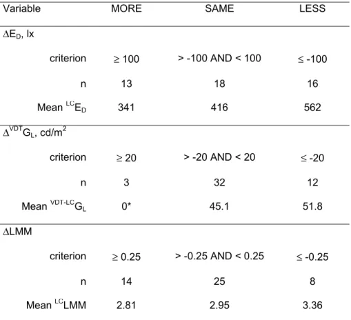
Three different categorical independent variables were chosen, each based on the photometric variables discussed earlier: ∆ED, ∆VDTGL, and ∆LMM. Each variable contained three categories labelled “MORE”, “SAME”, and “LESS”; the assignment to these variables is shown in Table 2. Also shown in Table 2 is the size of each category, and relevant mean luminous conditions prevailing during the day for each category. Note that these categories, inevitably, are not independent of absolute photometric variables; for example, those who chose an illuminance 100 lx or more higher than that which they experienced during the day (“MORE” category) also experienced the lowest illuminance during the day, on average.
The effect of each independent variable on each set of dependent variables was addressed in a separate MANOVA. Within each MANOVA two contrasts were of interest:
1. Comparing those participants who wanted a substantial change (“MORE” and “LESS” together) vs. those who did not (“SAME”). It was expected that this contrast would show strong effects on satisfaction and related outcomes.
2. Comparing those who wanted a substantial reduction (“LESS”) vs. those who did not (“MORE” and “SAME” together). It was expected that this contrast would show the strongest effects on outcomes influenced by glare.
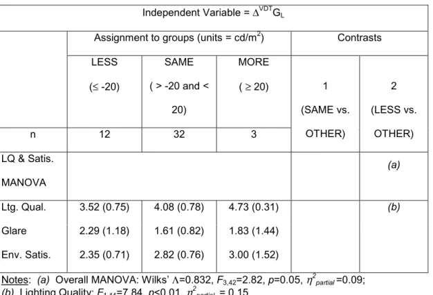
Only those MANOVAs related to mood, ratings of the lit environment and
environmental satisfaction were statistically significant and only in relation to ∆ED and ∆VDTGL. The results of the significant MANOVAs are shown in Tables 3 and 4. Graphs of the mean ratings associated with the univariate effects are shown in Figures 6(a)-(d). Within the MANOVA related to mood there was a significant univariate effect of Pleasure in Contrast 1 on ∆ED (η2partial=0.13); those who experienced lighting
conditions closest to their own choices had a significantly higher Pleasure rating. Within the MANOVA related to the lit environment and environmental satisfaction there were significant univariate effects of Lighting Quality (η2 partial =0.15) and Overall
Environmental Satisfaction (η2 partial =0.13) in Contrast 1 on ∆ED. Those who experienced lighting conditions closest to their own choices had significantly higher ratings of Lighting Quality and general Environmental Satisfaction. There was also a significant univariate effect of Lighting Quality (η2 partial =0.15) in Contrast 2 on ∆
VDT GL.
Those who substantially lowered the VDT screen glare image luminance at the end of the day had a significantly lower rating of Lighting Quality.
5 Discussion
Figures 3, 4 and 5 clearly show that occupants do respond to the lighting conditions they experience, and will express a desire for change if the prevailing conditions are not to their liking. Although we know that people adapt well to the lighting conditions they experience and will report satisfaction over a wide range (4,7), this does not mean that they do not express a preference for something different when offered the chance. If people were perfectly adaptive (or insensitive, or habituated) the regression lines in Figures 3, 4 and 5 would have been horizontal lines at y = 0.
5.1 Regressions for preferred illuminance
As described earlier, the regression-type analysis used here can be used to derive a preferred (or “ideal”) illuminance for the sample population studied. Discussion will first focus on the linear regressions in Figures 3 and 4(b). In Figure 3 the regression line crosses the x-axis at 392 lx. In other words, given a linear relationship, the
average respondent would not want any change in ED if they had experienced an ED of 392 lx during the day. Recall, however, that it was strongly suspected that this
illuminance selection was not the result of illuminance preference alone, but primarily the result of lighting choices to reduce VDT-screen glare. The regression shown in Figure 4(b) is after the effect of glare has been removed. In this case the point at which the linear regression line crosses the x-axis is 458 lx. This analysis provides
values for preferred ED independent of glare preferences. Therefore, it appears that although the preferred ED is around 460 lx (Figure 4(b)) people will lower this to around 400 lx to avoid glare (Figure 3). Interestingly, 460 lux is close to the mean value of LCE
D (actual value = 445 lx (10-12)). There were no systematic differences between the LC and NC groups on important demographic variables (10,12) (age and sex were controlled by matching the pairs) and therefore one would expect the illuminance preferences of the two groups to be the similar. One interpretation of this observation is that the LC participants were also trying to achieve 460 lx on the desktop, but, because they lacked prolonged experience of the space, did it in a way that created some VDT-screen glare.
Despite the appeal of a single preferred illuminance as provided by a linear regression, experience suggests occupant satisfaction is high over a range of illuminances. Further, when designing for illuminance in a large space for a large number of occupants, a single illuminance target would clearly be impractical to achieve. Even for a regular array of luminaires there is considerable variation in illuminance between locations below luminaires and locations between luminaires. In addition, differences in workstation furniture lead to even greater local variations in illuminance. The 3rd -order polynomial regression in Figure 4(b) provides a more practical range of preferred luminances (and also fits the data better than the linear regressions). For the 3rd-order regression, preferred ED is indicated not by the point at which the curve crosses the x-axis, but by the range of illuminances over which the curve is horizontal and close to zero. The range of preferred ED is 200 to 500 lx for the 3rd-order curve in Figure 4(b). This range conforms well with the 200 to 500 lx range recommended for most office work in the IESNA Handbook (15) and the CIBSE Code for Interior Lighting (16), and the
recommendations in IES RP-1 (17) and CIBSE LG7 (18) that desktop illuminance be less than 500 lx in VDT spaces.
5.2 Regressions for preferred luminance ratio
Figure 5(c) suggests a preferred maximum-to-minimium luminance ratio of 19.6. At first sight this number appears very high compared to values in standards and recommended practices (17,18), yet the lighting choices made by the participants were not, in general, anything out of the ordinary (12). Although standards and
recommended practices do not explicitly state how these luminance ratios are to be measured (15-18), the implication is that they are derived from spot luminances at the centre of easily-defined surfaces (e.g., partitions, desktop, computer screen). This method severely restricts the range of measured luminances, leading to relatively low luminance ratios (of the order of 3:1). For the measurements in this experiment a digitial video photometer was used to look at a grid of squares of approximately 1° (15 x 15 pixels) in size. We took the mean luminance of each square in the field of view, and compared the maximum square to the minimum square. This method will clearly yield a much greater range of luminance values and luminance ratios.
Nevertheless, the two methods are not necessarily inconsistent. Standards and recommended practices (17,18) do allow for small areas of higher luminance away from the traditional spot measurement locations. Such small areas can create accents and interest, whereas larger areas of the same luminance may be bothersome. Loe et al.(19) carried out an experiment in which participants assessed a variety of lighting
installations in a mock-up office. The photometric measurements taken in Loe et al.’s experiment with respect to luminance and luminance ratio were very similar to the measurements made in this paper. From their results, Loe et al. suggested that the maximum-to-minimum luminance ratio in the field of view be between 10 and 50. They plotted a composite subjective rating factor related to “Visual Interest” vs. luminance ratio and found a strong relationship. As maximum-to-minimum luminance ratio increased so did visual interest, but with diminishing returns. It is interesting to note that Loe et al.’s curve starts to level off at a ratio of about 20, similar to optimum value suggested in this paper.
5.3 Satisfaction and performance analyses
There were four significant univariate effects associated with significant MANOVAs. They are entirely consistent, and in the expected direction. Pleasure (mood), Lighting Quality rating, and Overall Environmental Satisfaction rating were all higher for those participants whose daytime desktop illuminance was within 100 lux of their own preferred choice at the end of the day, compared to those whose preferred choice differed from what they experienced during the day by more than ±100 lux. In other words, those participants who experienced conditions closest to what they would have chosen for themselves had higher ratings.
Lighting Quality rating was lower for those participants who experienced a glare image with a luminance more than 20 cd/m2 greater than their own preferred choice,
the day by less than 20 cd/m2 or those who expressed a preference for a higher luminance. The inference is that those participants who judged the glare image bothersome (irrespective of its absolute value) – and expressed this by lowering screen glare when they had the opportunity – had lower ratings of lighting quality.
In previously-reported analyses, the opportunity to choose luminous conditions at the start of the day did not lead to improved mood, satisfaction, or task performance in the LC participants, as had been expected (10,11). However, the analyses reported here show that experiencing the luminous conditions that one prefers improves satisfaction and increases pleasure. This finding provides some support to the theory that
preferred luminous conditions can increase positive affect (9). The size of the mood and satisfaction effects reported here is large, according to commonly-accepted standards (20), and is larger than subjective effects of this kind typically reported in the lighting literature.
The categorical analysis of luminous conditions relative to preference that produced these results is potentially confounded by absolute luminous conditions. However, this potential confound is somewhat allayed by the fact that previous analyses of the same dependent variables vs. absolute photometric variables found little(10).
Focussing now on ED, the results of this analysis indicate that there is a satisfaction benefit to be gained by providing occupants with an illuminance within 100 lx of the illuminance they would choose for themselves. Such a satisfaction benefit should be considered important in VDT offices, where employees represent around 90% of the cost of running a building – there are few that would argue that a more satisfied
employee is not an asset to his/her organisation. With this in mind, we returned to our data to derive the fraction of participants at any given ED who would have been within 100 lx of their own chosen illuminance; this is shown in Figure 7. There is a peak around 475 lx and a roughly-defined plateau between 275 lx and 600 lx. This could also be used as a basis for deriving recommended illuminance conditions for VDT offices. It is also interesting to note that no more than 40-50% of occupants can ever be within 100 lx of their preferred condition, with its associated satisfaction benefit, no matter what fixed illuminance is chosen. Here is a reason for providing individual control over lighting conditions.
5.4 Advantages of this Method
One can derive preferred luminous conditions by simply recording the choices people make when they have the choice and taking the mean or median. These data were recorded in this experiment for both LC and NC participants. However, the method described in this paper has three advantages:
1. Using regression one can separate preference effects, e.g., the effect of glare preference from illuminance preference;
2. The desire for change when the luminous conditions are not at preferred levels can be predicted; and,
3. Desire for change in luminous conditions appears to be a better predictor of mood and satisfaction than absolute measures of luminous conditions. Therefore this method may offer a more sensitive approach for investigating subjective effects of lighting quality.
5.5 Future work
This paper introduces a promising new method to objectively determine preferred photometric conditions. Although this paper focuses on desktop illuminance and maximum-to-minimum luminance ratio because of their widespread use, this same technique could be applied to other photometric variables of interest. However, despite the promise of the technique, it needs to be examined further before being considered as the basis for formal recommendations. This experiment was not designed with this analysis method in mind, and it therefore has its limitations.
The lighting conditions created by the LC participants were not evenly distributed across the range of interest. For example, there were few illuminance choices below 300 lux, and therefore few low illuminances experienced by NC participants (see Figure 3). This places some doubt on the reliability of the regression equations at low illuminances. Future work should fill in this gap, exposing a greater number of participants to low illuminance conditions.
Also, it is not clear that in making their choices at the end of the day, the NC participants reacted principally to illuminance or glare preferences. For this paper it was assumed, based on the comments of participants, that glare was the main driving photometric variable, and therefore its effect was partialled out first. Nevertheless, there remains a significant, although smaller, effect independent of screen glare that appears to be illuminance driven. A future experiment should separate the glare and illuminance influences not just statistically, but physically. It should be possible to
create a variety of lit environments in which desktop illuminance, screen glare, and partition luminance are more independent than they were in this experiment.
Further, the data described in this paper were obtained from a single, windowless space with a specific collection of lighting equipment. Similar data need to be collected in different spaces with different lighting designs.
Related to this latter point, all lighting choices were made from a fixed starting point, which featured the dimmers at about half their maximum settings and the task light on, generating about 500 lux on the desktop. Although participants were introduced to a wide variety of possibilities when the lighting control system was being demonstrated to them, it is still possible that the choices made were influenced by this initial setting; in psychology this phenomenon is known as anchoring. This effect can easily be investigated in the future, by exposing independent groups of participants to different starting points. Any effect can then be statistically removed from the data prior to examining illuminance and luminance preferences.
In the analysis of satisfaction data, we created new independent categorical variables based on deviation from preferred luminous conditions. However, this assignment was not independent of the absolute luminous conditions experienced during the day. Independence in this experiment was not possible, given the experimental design and the sample size. A future experiment could achieve such independence by exposing a large sample to the same luminous conditions before allowing them to choose their own lighting.
Finally, the possibility that end of day lighting choices were tempered by habituation cannot be discounted. That is, end of day lighting choices were not entirely driven by lighting preferences, but also by becoming accustomed to conditions experienced during the day. This might also explain why the preferred illuminance for the NC participants derived by linear regression is close to the mean illuminance during the day. Habituation will act to reduce the slope of the linear regressions, perfect habituation would reduce the slope to zero. Shortening exposure to initial lighting conditions prior to making a lighting preference choice should reduce habituation effects (though it would also reduce the experience from which occupants could make an informed choice) – this could be examined in a future experiment.
The experimental methods suggested by this approach can be extended to provide a strong test of the positive affect theory of lighting-behavioural effects. The effect size observed in this study is large enough to warrant such attention. Despite this size, the degree of change in mood and satisfaction achieved by the discrepancy between preferred and experienced lighting conditions was insufficient to cause statistically-significant changes in other dependent variables, such as complex task performance, that other researchers have observed with other ways of changing positive affect (21, 22). A replication with a larger range of luminous conditions (and more discrepancy
between preferred and experienced luminous conditions), more sensitive tasks, and a larger sample size would advance our understanding of this potentially important psychological mechanism.
Conclusions
Bearing in mind the limitations on this work described in the previous section, the following conclusions can be drawn from this experiment:
• Preference for a change in lighting at the end of the day is correlated to the lighting condition experienced during the day.
• Preference for change is driven by VDT screen glare experienced, by desktop illuminance experienced, and by luminance ratio experienced.
• Using a regression method, the preferred desktop illuminance range for a population in a VDT office is around 200 to 500 lux.
• The preferred maximum-to-minimum luminance ratio in the field of view is around 20 to 1.
• Participants experiencing lit environments substantially different from their preferred lit environment have significantly lower ratings of Pleasure (mood), Lighting Quality, and Overall Environmental Satisfaction.
• By maximising the number of occupants receiving within 100 lx of their own preferred illuminance, the recommended range in a VDT office is 275 to 600 lx. Note, however, that no more than 40-50% of occupants will be within 100 lx of their preference no matter what fixed illuminance is chosen.
These points provide the designer with some interesting information. Firstly, the research provides empirical evidence to support the recommendations for illuminance and luminance in guides for office lighting(15-18). The lighting preferences of the
participants in this experiment, as a group, tended to match the current
recommendations quite well. Nevertheless, the behavioural data suggests intriguing supplementary information. A close match between an individual’s own lighting preferences and the lit environment they experience correlates with increased
environmental satisfaction. For the majority who believe that an organisation benefits from employees who are more satisfied with their environment this is an important finding. However, the data also suggests that no fixed lit environment can match the illuminance preferences of more than around 50% of occupants. Only some form of individual control would allow all occupants to match local lighting conditions to their own preferences.
Appendix
This Appendix contains tables detailing the final models for predicting ∆ED. The information given here in tabular format complements that shown in graphical format in Figure 4. Each table gives the additional variance in ∆ED explained (∆R
2
) when a variable (or block of variables) is added to the model. In all cases, the first predictor entered into the model accounts for changes in screen glare conditions at the end of the day (consistent with the “partialling out” process described in the main body of the paper). Models with a both a linear (Table A1) and cubic (Table A2) relationship to LC
ED are shown. In the case of the cubic relationship, LCED, LCED2, LCED3, are added to the model at the same time; i.e., the best linear combination of LCED, LCED2, LCED3 is used as a single predictor.
At the bottom of each Table is the total variance in ∆ED explained by the model (Σ R2). Also shown is Σ R2adj, which compensates for the number of predictors used in the
Table A1. Model predicting ∆ED from ∆VDTGL and linear components of LCED.
Variables added (in order) Standard. coefficient df p ∆ R2 ∆VDTGL 0.495 1, 44 <0.01 0.44 LCE D -0.450 1, 44 <0.01 0.18 Σ R2 0.61 Σ R2adj 0.59
Table A2. Model predicting ∆ED from ∆VDTGL and cubic components of LCED.
Variables added (in order) Standard. coefficient df p ∆ R2 ∆VDTGL 0.445 1, 42 <0.01 0.44 LCE D, LCED2, LCED3, -2.205, 6.167, -4.568 3, 42 <0.01 0.30 Σ R2 0.73 Σ R2adj 0.71
Acknowledgements
The preparation of this paper was supported by the Canadian Electrical Association (Agreement No. 9433 U 1059), Natural Resources Canada, the Panel on Energy Research and Development, and the National Research Council of Canada (NRC), as part of the NRC project “Experimental Investigations of Lighting Quality, Preferences, and Control Effects on Task Performance and Energy Efficiency” (A3546). Lighting equipment used in this experiment was donated by CANLYTE Inc., General Electric Co., Ledalite Architectural Products Inc., Litecontrol Corp., Luxo Lamp Ltd., Osram-Sylvania Inc., Peerless Lighting Ltd, and Philips Lighting. We are especially grateful to our colleagues at IRC and elsewhere, for their contributions: Jana Svec and Steffan Jones for their work as experimenters; Ralston Jaekel, Roger Marchand and Marcel Brouzes for technical assistance; Vilayvanh Sengsouvanh for conducting pilot tests; Jennifer Roberts for additional data management; and, Sherif Barakat, Dale Tiller, Kevin Houser and Terry McGowan for advice.
References
1 Collins B L Discussion (re: Illuminance selection based on visual performance -- and other fairy stories) Journal of the Illuminating Engineering Society 25(2) 48 (1996)
2 Boyce P R Lighting research and lighting design: bridging the gap Lighting Design and Application, 17(5), 10-12, 50-51 (1987, May) and 17(6), 38-44 (1987, June)
3 Mills E and Borg N Trends in recommended illuminance levels: an international comparison [Abstract] Journal of the Illuminating Engineering Society 27(2) 178 (1998)
4 Boyce P R Illuminance selection based on visual performance - and other fairy stories Journal of the Illuminating Engineering Society 25(2) 41-49 (1996) 5 Veitch J A and Newsham G R Determinants of lighting quality I: state of the
science Journal of the Illuminating Engineering Society 27(1) 92-106 (1998) 6 Veitch J A and Newsham G R Determinants of lighting quality II: Research
and recommendations Paper presented at the 104th Annual Convention of the American Psychological Association Toronto Ontario Canada (1996, August) (ERIC Document Reproduction Service No. ED408543)
7 Boyce P R Lighting quality: The unanswered questions In J A Veitch (Ed.) Proceedings of the First CIE Symposium on Lighting Quality (CIE x015-1998) 72-84 (Vienna, Austria: Commission Internationale de l'Eclairage) (1998) 8 Veitch J A Julian W and Slater A I A framework for understanding and
promoting lighting quality In J A Veitch (Ed.) Proceedings of the First CIE Symposium on Lighting Quality (CIE x015-1998) 237-241 (Vienna, Austria: Commission Internationale de l'Eclairage) (1998)
9 Baron R A Rea M S and Daniels S G Effects of indoor lighting (illuminance and spectral distribution) on the performance of cognitive tasks and interpersonal behaviors: the potential mediating role of positive affect Motivation and Emotion 16 1-33 (1992)
10 Veitch J A and Newsham G R Experimental investigations of lighting quality, preferences and control effects on task performance and energy efficiency: experiment 2 primary analyses IRC Internal Report No. 767 (1998)
11 Veitch J A and Newsham G R Exercised control, lighting choices, and energy use: An office simulation experiment Journal of Environmental Psychology 20 219-237 (2000)
12 Veitch J A and Newsham G R Preferred luminous conditions in open-plan offices: research and practice recommendations Lighting Research and Technology (in press) (2000)
13 Newsham G R, Veitch J A and Tiller D K Software tools to evaluate occupant satisfaction and performance Proceedings of Healthy Buildings/IAQ 97 Conference pp 207-212 (Bethesda) (1997)
14 Schiller G, Arens E, Bauman F, Benton C, Fountain M, Doherty T and Craik K A field study of thermal environments and comfort in office buildings ASHRAE Final Report No. 462-RP (1988)
15 Illuminating Engineering Society of North America (IESNA) Lighting Handbook (Ed: Rea M) pp.460, 463 (New York: IESNA) (1993).
16 Chartered Institution of Building Services Engineers Code for interior lighting (London, UK: CIBSE) (1994)
17 Illuminating Engineering Society of North America (IESNA) American national standard practice for office lighting ANSI/IESNA-RP-1-1993 (New York: IESNA) (1993)
18 Chartered Institution of Building Services Engineers Lighting for offices (Lighting Guide LG7: 1993) (London, UK: CIBSE) (1993)
19 Loe D L, Mansfield K P and Rowlands E Appearance of lit environment and its relevance in lighting design: experimental study Lighting Research and Technology 26(3) 119-133 (1994)
20 Cohen J Statistical power analysis for the behavioral sciences (2nd ed.). (Hillsdale, NJ: Erlbaum) (1988)
21 Isen A M Positive affect, cognitive organization, and social behavior In L Berkowitz (Ed.) Advances in experimental social psychology (Vol. 21) pp. 203-253 (New York: Academic Press) (1987)
22 Baron R A and Thomley J A whiff of reality: Positive affect as a potential mediator of the effects of pleasant fragrances on task performance and helping. Environment and Behavior, 26, 766-784 (1994)
23 Houser K W Tiller D K and Pasini I C Toward the accuracy of lighting simulations in physically based computer graphics software Journal of the Illuminating Engineering Society of North America 28(2) 117-129 (1999)
Table 1 Measured room surface reflectances
Room Surface Material Colour Reflectance
ceiling acoustic tile matte white .89
partition fabric matte light grey .46
partition frame enamel paint low gloss light grey .47
VDT screen (off) specular glass black .12
desk top Formica low gloss light grey .50
binder bin Formica low gloss maroon .07
floor carpet tile matte multi-colour (dark grey base) .12
Note. From Houser et al.(23) The space these authors modelled was the same space,
Table 2. Conditions for assigning the individual values of each independent variable to categories, with sample sizes and relevant mean luminous conditions during the day for each category.
Variable MORE SAME LESS
∆ED, lx criterion ≥ 100 > -100 AND < 100 ≤ -100 n 13 18 16 Mean LCED 341 416 562 ∆VDTGL, cd/m2 criterion ≥ 20 > -20 AND < 20 ≤ -20 n 3 32 12 Mean VDT-LCGL 0* 45.1 51.8 ∆LMM criterion ≥ 0.25 > -0.25 AND < 0.25 ≤ -0.25 n 14 25 8 Mean LCLMM 2.81 2.95 3.36
Table 3. Results of significant MANOVAs related to ∆ED. Each significant MANOVA is followed by each of its univariate tests, significant or not. Cells associated with
univariate tests show group means, with standard deviations in parentheses. Notes below the table refer to letters in the Contrasts columns; there is a letter if the test associated with that contrast is significant.
Independent Variable = ∆ED
Assignment to groups (units = lx) Contrasts LESS (≤ -100) SAME ( > -100 and < 100) MORE ( ≥ 100) n 16 18 13 1 (SAME vs. OTHER) 2 (LESS vs. OTHER) Mood MANOVA (a) Pleasure 4.23 (1.53) 5.71 (1.54) 4.55 (2.09) (b) Arousal 3.26 (1.34) 3.36 (1.33) 3.43 (1.43) Dominance 3.74 (1.35) 4.65 (1.24) 4.15 (1.14) LQ & Satis. MANOVA (c) Ltg. Qual. 3.80 (0.77) 4.37 (0.53) 3.65 (0.98) (d) Glare 2.19 (1.09) 1.56 (0.78) 1.65 (1.01)
Env. Satis. 2.44 (0.80) 3.08 (0.60) 2.54 (0.92) (e)
Notes: (a) Overall MANOVA: Wilks’ Λ=0.797, F3,42=3.56, p<0.05, η
2
ave=0.07;
(b) Pleasure: F1,44=6.66, p<0.05, η2partial = 0.13; (c) Overall MANOVA: Wilks’ Λ=0.805,
F3,42=3.36, p<0.05, η2partial =0.11; (d) Lighting Quality: F1,44=7.99, p<0.01, η2partial =
0.15; (e) Environmental Satisfaction: F1,44=6.66, p<0.05, η
2
Table 4. Results of significant MANOVAs related to ∆VDTGL. Each significant
MANOVA is followed by each of its univariate tests, significant or not. Cells associated with univariate tests show group means, with standard deviations in parentheses. Notes below the table refer to letters in the Contrasts columns; there is a letter if the test associated with that contrast is significant.
Independent Variable = ∆VDTGL
Assignment to groups (units = cd/m2) Contrasts LESS (≤ -20) SAME ( > -20 and < 20) MORE ( ≥ 20) n 12 32 3 1 (SAME vs. OTHER) 2 (LESS vs. OTHER) LQ & Satis. MANOVA (a) Ltg. Qual. 3.52 (0.75) 4.08 (0.78) 4.73 (0.31) (b) Glare 2.29 (1.18) 1.61 (0.82) 1.83 (1.44) Env. Satis. 2.35 (0.71) 2.82 (0.76) 3.00 (1.52)
Notes: (a) Overall MANOVA: Wilks’ Λ=0.832, F3,42=2.82, p=0.05, η2partial =0.09;
(b) Lighting Quality: F1,44=7.84, p<0.01, η
2
Figure Captions
Figure 1(a). Layout of furniture and reflected ceiling in mock-up office. Numbers indicate the individual circuits described in text.
Figure 1(b). Relationship between dimmer setting (number of LEDs lit) and relative light output, for the recessed parabolic fixtures .
Figure 2. Key photometric variables referred to in this paper. LMM, VDTG%, VDTGL, were determined using a video photometer. LMM did not include the VDT screen.
Figure 3. Change in desktop illuminance chosen by NC participants (∆ED) vs. desktop illuminance they experienced during the day (LCED).
Figure 4(a). Change in desktop illuminance chosen by NC participants (∆ED) vs. change in glarespot luminance chosen (∆VDTGL). (b) Residual of change in desktop illuminance chosen by NC participants after effect of glarespot luminance change is removed vs desktop illuminance experienced during the day (LCED). Linear and 3rd -order polynomial regressions are shown.
Figure 5(a). Change in log of luminance ratio chosen by NC participants (∆LMM) vs. log of luminance ratio they experienced during the day (LCLMM). (b) Change in log of luminance ratio chosen by NC participants (∆LMM) vs. change in glarespot luminance chosen (∆VDTGL). (c) Residual of change in log of luminance ratio chosen by NC participants after effect of glarespot luminance change is removed vs log of luminance ratio experienced during the day (LC∆LMM). Linear regression is shown.
Figure 6. Graphs of significant univariate effects when mood, satisfaction and performance outcomes were analysed with respect to end-of-day changes in photometric variables.
Figure 7. Fraction of participants who would be within 100 lx of their chosen desktop illuminance (ED), for any given ED.
1 1 1 1 1 1 2 2 2 2 2 2 2 2 2 2 3 3 3 3 3 3 3 3 WS2 WS5 4 4 4 4 4 4 1 1 1 1 Figure 1(a)
0.0
0.2
0.4
0.6
0.8
1.0
0
2
4
6
8
10
12
14
16
Dimmer LED setting
R
e
la
tiv
e
li
ght output
Figure 1(b)VDTG
% is percent of VDT screen area > 40 cd/m2, when screen is off. VDTGL is the mean luminance of these areas.
ED is illuminance measured on the desktop, on the side opposite the task light. LMM is natural log of
the ratio of max. to min. luminance in the shaded area (rectilinear approx. of field of view of occupant seated at computer, ~35-40o tall); values
averaged over target approx. 1° square
y = -0.8497x + 333.42 R2 = 0.3978 -600 -400 -200 0 200 400 600 0 100 200 300 400 500 600 700 800 Day's illuminance, LCEd (lx)
Illuminance change chosen by NC,
∆∆∆∆
Ed
(lx)
y = 4.5677x - 1.0088 R2 = 0.4348 -800 -600 -400 -200 0 200 400 600 -80 -60 -40 -20 0 20 40 60 80
Glarespot luminance change chosen by NC, ∆∆G∆∆ L (cd/m 2 ) Illum ina nc e c h a nge c hos e n by N C , ∆∆∆∆ Ed (l x)
(a)
y = -0.5372x + 245.93 R2 = 0.2811 y = -8E-06x3 + 0.0086x2 - 2.7736x + 327.58 R2 = 0.4732 -600 -400 -200 0 200 400 600 0 100 200 300 400 500 600 700 800 Day's illuminance, LCEd (lx) R e s idua l of ∆∆∆∆ Ed , effect o f ∆∆∆∆ GL remo ved (l x) y = -0.5372x + 245.93 y = -8E-06x3 + 0.0086x2 – 2.7736x + 327.58(b)
Figure 4 (a) Figure 4 (b)y = -0.8006x + 2.4556 R2 = 0.2603 -1.5 -1.0 -0.5 0.0 0.5 1.0 1.5 2.0 2.5 3.0 3.5 4.0
Day's LN(lum. Ratio), LCLMM
C h a nge in LN (l um . ra ti o) c hos e n by N C , ∆∆∆∆ LMM y = -0.0075x + 0.0014 R2 = 0.2409 -1.5 -1.0 -0.5 0.0 0.5 1.0 1.5 -80 -60 -40 -20 0 20 40 60 80
Glarespot luminance change chosen by NC, ∆∆∆∆GL (cd/m 2 ) C h a nge in LN (l um . ra ti o) c hos e n by N C , ∆∆∆∆ LMM
(a)
(b)
Figure 5 (a) Figure 5 (b)y = -0.6883x + 2.0482 R2 = 0.2535 -1.5 -1.0 -0.5 0.0 0.5 1.0 1.5 2.0 2.5 3.0 3.5 4.0
Day's LN(lum. Ratio), LCLMM
Residual of ∆∆∆∆ LMM, effect of ∆∆∆∆ GL r e moved
(c)
Figure 5 (c)DIFF SAME CONTRAST1$ 0 1 2 3 4 5 6 7 8 P L E A S 2 CONTRAST 1 ON ∆ED