HAL Id: hal-00304770
https://hal.archives-ouvertes.fr/hal-00304770
Submitted on 1 Jan 2003HAL is a multi-disciplinary open access archive for the deposit and dissemination of sci-entific research documents, whether they are pub-lished or not. The documents may come from teaching and research institutions in France or abroad, or from public or private research centers.
L’archive ouverte pluridisciplinaire HAL, est destinée au dépôt et à la diffusion de documents scientifiques de niveau recherche, publiés ou non, émanant des établissements d’enseignement et de recherche français ou étrangers, des laboratoires publics ou privés.
J. P. Whiting, M. F. Lambert, A. V. Metcalfe
To cite this version:
J. P. Whiting, M. F. Lambert, A. V. Metcalfe. Modelling persistence in annual Australia point rainfall. Hydrology and Earth System Sciences Discussions, European Geosciences Union, 2003, 7 (2), pp.197-211. �hal-00304770�
197
Modelling persistence in annual Australian point rainfall
Julian P. Whiting
1, Martin F. Lambert
1and Andrew V. Metcalfe
21Centre for Applied Modelling in Water Engineering, School of Civil and Environmental Engineering, University of Adelaide, Adelaide 5005, Australia 2Department of Applied Mathematics, University of Adelaide, Adelaide 5005, Australia
Email for corresponding author: [email protected]
Abstract
Annual rainfall time series for Sydney from 1859 to 1999 is analysed. Clear evidence of non-stationarity is presented, but substantial evidence for persistence or hidden states is more elusive. A test of the hypothesis that a hidden state Markov model reduces to a mixture distribution is presented. There is strong evidence of a correlation between the annual rainfall and climate indices. Strong evidence of persistence of one of these indices, the Pacific Decadal Oscillation (PDO), is presented together with a demonstration that this is better modelled by fractional differencing than by a hidden state Markov model. It is shown that conditioning the logarithm of rainfall on PDO, the Southern Oscillation index (SOI), and their interaction provides realistic simulation of rainfall that matches observed statistics. Similar simulation models are presented for Brisbane, Melbourne and Perth.
Keywords: Hydrological persistence, hidden state Markov models, fractional differencing, PDO, SOI, Australian rainfall
Introduction
Various studies have identified the influence of the El Niño/ Southern Oscillation (ENSO) phenomenon upon the Australian climate and in particular on its rainfall. Although being a process shown to have global effects, the axis of ENSO is the tropical Pacific Ocean, where strong ocean-atmosphere interactions can produce climatic changes that have been linked to rainfall across Australia. Chiew et al. (1998) describe the Southern Oscillation as a ‘see-saw’ of atmospheric pressure differences between the Australian-Indonesian region and the eastern tropical Pacific Ocean. The strength and frequency of the El Niño phenomenon is modulated by anomalies in Pacific sea surface temperatures. McBride and Nicholls (1983) showed that the variability of rainfall across Australia is strongly influenced by ENSO on interannual time scales.
El Niño events bring shifts in the circulation patterns of the Australian climate systems, which can be monitored by differences in both air pressure and temperature. One of the most commonly used indicators of ENSO variability is the Southern Oscillation Index (SOI), which is a measure of the normalised monthly anomalies of the difference between the mean sea level pressures in Darwin, Australia and Tahiti. Alternative indicators of the El Niño phenomenon are direct
measurements of anomalous sea surface temperatures (SSTs), such as the NINO3 index, which the International Research Institute for Climate Research defines as being measured in the region 5oN–5oS, 90oW–180oW of the
Pacific.
The effects of ENSO vary on inter-decadal time-scales (e.g. Allan et al., 1996). Furthermore, various studies (e.g. Zhang et al., 1997) demonstrate an inter-decadal variability in patterns of Pacific sea surface temperatures that is associated with variations in Australian rainfall (e.g. Latif et al., 1997). This anomalous warming and cooling of the Pacific Ocean, termed the Interdecadal Pacific Oscillation (IPO) influences the ENSO phenomenon in Australia (Franks, 2002). Results published by Power et al. (1999) suggest that the influence of ENSO upon the Australian climate fluctuates on inter-decadal time-scales in connection with the IPO. Chiew and McMahon (2003) demonstrate a link between ENSO and Australian rainfall and streamflow for 284 catchments throughout Australia.
Mantua et al. (1997) identified a multi-decadal persistence in North Pacific sea surface temperatures, termed the Pacific Decadal Oscillation (PDO), which has been correlated to weather patterns across North America. This climate index was derived from an approach that was independent of
methods used to obtain the IPO time series, although Franks (2002) indicates that the two indices are highly correlated. This correlation increases confidence that the two approaches are reflecting legitimate variability in the climate. To investigate the influence of climatic variability on annual rainfall in this paper, the PDO index has been used in place of the IPO, as stronger relationships were found when using this index.
When observing Australian rainfall on a regional scale, Simmonds and Hope (1997) identified statistically significant persistence on monthly, seasonal and annual time-scales, together with significant correlation with SOI. This paper will assess whether there are any practically important correlations with climate systems in the point rainfall time series of selected Australian capital cities, and if so, whether these are useful for simulations of rainfall. Simulated rainfall is needed for diverse purposes such as reservoir design, assessment of control systems for the release of water from reservoirs, and flood defences.
Analysis of point rainfall
SEASONAL PATTERN AND TREND
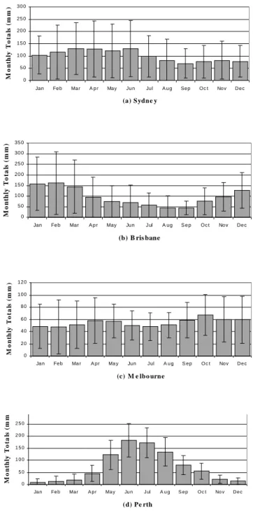
Long-term continuous rainfall data, recorded at monthly intervals were available for four Australian capital cities: Sydney (1859–1999), Melbourne (1856–1999), Brisbane (1860–1996) and Perth (1876–1991). Monthly rainfall totals were added to obtain time series of anual rainfall totals for each of these cities. Some statistics from these annual data are shown in Table 1.The location of these cities indicate the variable climatic conditions that exist along the Australian coast.This variation is demonstrated in Fig. 1 which indicates the different distributions of monthly rainfall totals for each of these cities. The large standard deviations of the monthly totals, indicated by the semi-lengths of the lines in Fig. 1 indicate high variability of rainfall in these Australian cities.
The seasonal shift of a belt of high air pressure that brings easterly-moving air disturbances over the Australian continent is the dominant force in the climate of this country
Table 1. Summary of rainfall data from selected Australian capital cities
Location BOM rain gauge Period Length Annual Statistics (mm)
identification number (Years) (Mean (sd))
Sydney 066062 Jan. 1859 – Dec. 1999 141 1226 (331)
Brisbane 040214 Jan. 1860 – Dec. 1993 134 1154 (358)
Melbourne 086071 Jan. 1856 – Dec. 1999 144 657 (129)
Perth 009034 Jan. 1876 – Dec. 1991 116 868 (162)
0 50 100 150 200 250 300
Jan Feb Ma r A p r May Jun Jul A ug Sep Oc t Nov Dec
(a) Sydne y M o n th ly T o ta ls (m m ) 0 50 10 0 15 0 20 0 25 0 30 0 35 0
Jan Fe b Mar A p r May Jun Jul A ug S e p Oc t No v De c (b) B ris bane M o n th ly T o ta ls (m m ) 0 20 40 60 80 100 120
Jan Feb Ma r A pr Ma y Jun Jul A u g S ep Oc t Nov Dec
(c) M e lbo urne M on th ly T o ta ls ( m m ) 0 5 0 1 0 0 1 5 0 2 0 0 2 5 0 Ja n Fe b Ma r A p r Ma y Ju n Jul A u g S e p Oc t No v De c (d) Pe rth M o nt hl y To ta ls ( m m)
Fig. 1. Monthly averages of rainfall data for selected Australian
capital cities; the heights of the bars are the mean monthly totals and the lines represent two standard deviations of monthly totals
199 (Harrison and Dodson, 1993). When located at 29–32o S in
winter, this system brings rainfall to the south of the continent in the form of Southern Ocean cold fronts. This pattern is contrasted with conditions in summer, during which the high-pressure belt moves further south to 37–38o
S, allowing tropical low-pressure systems to influence the country, bringing hot, dry conditions to the south of the continent and summer rainfall to the north. This northern Australian summer rain is derived from the influence of tropical monsoonal airflows originating in the Pacific.
The predominantly summer distribution of rainfall in Brisbane, shown in Fig. 1b can be contrasted with the strong winter rainfall distribution in Perth, Fig. 1d, both of which indicate the influence of this high pressure belt on the distribution of rainfall. The rainfall records in both Sydney (Fig. 1a) and Melbourne (Fig. 1c) show more uniform distributions across the twelve calendar months than either Brisbane or Perth. The climate of Sydney, situated on the eastern coast of Australia at latitude of approximately 34o,
is influenced by both moist easterly winds from the Pacific and Southern ocean air flows. Melbourne, situated further south than Sydney, at latitude 37o S, is under less influence
from the tropical systems of the Pacific and is thus affected by Southern Ocean cold fronts for much of the year. NON-STATIONARITY IN RAINFALL TIME SERIES Figure 2a– d show the rainfall time series for the four cities. The regression of annual rainfall {xt} on time (t, in years from start of record) is shown in Table 2 for each city. Although there is no evidence of a consistent linear trend over the past century, the time series plot for Sydney, Fig. 2a, shows periods during which rainfall is either consistently above or below the long-term mean value. In particular, the 40-year period between 1905 and 1944 shows a reduction in both the mean annual rainfall and the variation about this mean. The mean annual rainfall in this period is 1096 mm compared to 1298 mm in the period 1945–1999 and 1252 mm prior to 1905. Similarly, the standard deviation of the period 1905–1944 is 235 mm compared to 349 mm for the period prior to this and 353 mm for the period following. This apparent step change in rainfall was discussed by Cornish (1977) and is associated with a dramatic increase in flood risk across New South Wales from 1945 (Franks, 2002).
CUSUM chart analysis is a standard technique used to show changes in the underlying mean of a system. The CUSUM were calculated from
(
)
∑
= − = t 1 k k t x x S (1) 2000 1500 1000 500 1985 1960 1935 1910 1885 1860 A n n u a l R a in fa ll ( mm) 1400 1300 1200 1100 1000 900 800 700 600 500 1980 1960 1940 1920 1900 1880 A n n u a l R a in fa ll ( m m) 1000 900 800 700 600 500 400 300 1985 1960 1935 1910 1885 1860 A n nu a l R a in fa ll ( mm) 2500 1500 500 1985 1960 1935 1910 1885 1860 A nnu a l R a in fa ll ( m m ) (a) (b) (c) (d)Fig. 2. Time series of annual rainfall in Sydney (a), Brisbane (b),
where x x n n 1 t t
∑
== and n is the number of years.
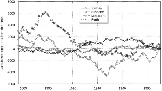
Positive slopes on these charts indicate a period of above average values (hence a ‘wet’ period in this context) with a negative slope indicating a below-average period. The rainfall time series for the four Australian capital cities clearly show periods during which the annual rainfall is either persistently below or above the long-term mean. The CUSUM charts for the four capital cities are shown together in Fig. 3, over the common length of 116 years (1876–1991), which can allow for the comparison of period changes between the various cities.
The number of statistically significant (2% level, Montgomery (1991) for example) changes in the mean for Sydney, Brisbane, Melbourne and Perth were 11, 7, 8 and 7 respectively. Table 3 shows the correlations between the annual rainfall time series in the four selected capital cities. The italicised values indicate correlations that are statistically significant at the 5% level.
Investigation of persistence in Sydney
rainfall
The time series plot of both the Sydney data and the Brisbane data show clear sustained changes in their mean level. The change in the annual Sydney data is now analysed in more detail.
AUTOCORRELATION AND SPECTRAL ANALYSIS An important guide to determining the properties of a time series is the correlation between data points at different intervals. The autocorrelation at lag k in a time series is estimated by
(
)(
)
(
)
∑
∑
= − = + − − − = N 1 t 2 t k N 1 t k t t x x x x x x r(k) (2)Correlations that decay very slowly to zero suggest that separated observations are related and ‘long-memory’ or
-6000 -4000 -2000 0 2000 4000 6000 8000 1880 1900 1920 1940 1960 1980 Sydney Brisbane Melbourne Perth C u mu la ti v e d e pa rt u re s f rom th e m e an
Table 2. Summary of regressions of annual rainfall on time Location Constant Coefficient Standard T-ratio P value
for t error
Sydney 1198 0.391 0.687 0.57 0.570
Brisbane 1218 -0.949 0.798 -1.19 0.237
Melbourne 654 0.035 0.259 0.14 0.892
Perth 887 -0.319 0.451 -0.71 0.481
Table 3. Correlations between annual rainfall time series in selected
capital cities
Location Brisbane Melbourne Perth
Sydney 0.424 0.190 0.038
Brisbane – 0.141 0.162
Melbourne – – 0.152
201 ‘long-range dependence’ is present. Beran (1994) provides
mathematical definitions of persistence in terms of both the correlogram and the spectrum of a time series. Persistence causes correlograms to decay hyperbolically, with r(k) approximating k-α as the lag increases. Time series can show both short term and long term correlations, in which case a fractional autoregressive integrated moving average model (FARIMA (p,d,q)), with the differencing parameter d between 0 and 0.5, is a suitable model. However, many hydrological time series can be modelled reasonably well by autoregressive processes of order 1 (AR(1) processes). These are characterised by a significantly large r1 value followed by an approximate exponential decay.
Figure 4 shows the correlogram with 5% lines of significance included. Since no correlations lie beyond these lines, there is no convincing evidence of persistence when the rainfall is aggregated at an annual level. Nor, with r(1) equal to just 0.10, r(3) equal to 0.14 and r(2) and r(4) being negative (equal to –0.01), is there any suggestion that an AR(1) model is appropriate.
The spectral density of a persistent stochastic process is asymptotic to the vertical, as the frequency tends to zero. The sample power spectrum can be estimated through a variety of methods. Estimated from the sample autocovariance, the smoothed sample spectrum was calculated from
( )
f 2 c( )
0 2 w( ) ( )
kckcos(2 fk) :0 f 0.5 C 1 M 1 k < ≤ + × =∑
− = π (3a) where( )
k(
x x)(
x x)
n c k n 1 t k t t∑
−= − + − = (3b) and( )
< ≤ − × < ≤ × + × − = M k 2 M : m k 1 2 2 M k 0 : m k 6 m k 6 1 k w 3 3 2 (3c)where M is the bandwidth of the window.
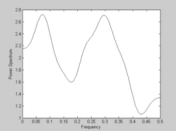
The sample power spectrum for the Sydney annual rainfall
data series, with M equal to2 n, is shown in Fig. 5. There is no suggestion of a peak at a frequency of zero, the two peaks correspond approximately to one cycle per 13 years and one cycle per three years.
Although CUSUM charts showed non-stationarity in the annual rainfall of Sydney, no convincing evidence of the 40-year ‘dry’ period (1905–1944) being indicative of long-term persistence was found in either autocorrelation or spectral analysis. These statistics do provide clear evidence of persistence in well known persistent time series such as the River Nile annual flows, which are well modelled by fractional differenced autoregressive (FAR) models (Beran, 1994). Hidden state Markov (HSM) models have been shown to provide realistic simulations of time series that appear to have jumps in the mean level. Such time series do not necessarily have marked autocorrelations; however they typically have Hurst coefficients that are significantly higher than realisations of independent variates (discrete white noise (DWN)).
HURST COEFFICIENTS
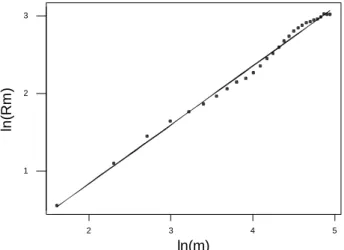
In results published in 1951, Hurst outlined his detection of long-range dependence in sequences of hydrological and geophysical data. In particular, this persistence was detected in the annual minima of the River Nile. By noticing in various series a tendency for deficits and surpluses of inflows to persist (Hurst, 1951), a statistic known as the rescaled adjusted range (Rm) was used to quantify the long-range dependence in the time series.
From the mean (x) of a time series (xt) of length n, the
adjusted partial sums (Sk), which are equivalent to cumulative sums, can be calculated for k=1,…,n as
∑
= − = k 1 t t k x kx S (4) 35 25 15 5 1.0 0.8 0.6 0.4 0.2 0.0 -0.2 -0.4 -0.6 -0.8 -1.0 Au to c o rre la ti o nFig. 4. Correlogram for the time series of annual rainfall in Sydney
(1859 – 1999)
Fig. 5. Power spectrum for the time series of annual rainfall in
The rescaled adjusted range, Rm, is the standardised difference between the maximum and minimum values of Sk over a ‘block’ size of length m < n as shown:
(
)
(
)
{
maxS,...,S minS,...,S}
sRm = 1 m − 1 m (5)
For each block size m, adjusted partial sums are successively generated at S2, S3,…, Sn-m, producing (n–m) values for each Rm. The average Rm is then determined for values of m taken at regular intervals up to a maximum of n. Beran (1994) provides details of estimation.
By plotting ln(Rm) against ln(m), where m is the block size of this statistic, the slope of the line around which data points are scattered is equivalent to H, the Hurst coefficient. This linear logarithmic relationship is equivalent to:
H
m m
R ∝ (6)
Persistence can be characterised by the rescaled adjusted range behaving as a function mH, H > ½ of the sample size
m, rather than as the m1/2 that is characteristic of
short-memory processes (Hosking, 1984). Sequences of independent Gaussian variables (sequences with an absence of long-term memory) will have a value of H of approximately 0.5 and higher values of H directly relate to a higher intensity of persistence.
The rescaled adjusted range for the Sydney annual rainfall time series was calculated at block sizes from 5 up to the record length of 141 years, and shown in Fig. 6. The estimate of the Hurst coefficient from this diagram is H=0.76, which is significantly higher than the 0.5 expected of an independent process (one-sided P≈0.02, from Monte Carlo simulation), providing evidence that the rainfall time series is persistent.
TWO-STATE HIDDEN STATE MARKOV (HSM) MODELS
Thyer and Kuczera (2000) applied the hidden state Markov (HSM) model to the simulation of annual rainfall time series in this country. An HSM model, which simulates data in either one of two climate states, is presented here as a method of data simulation that may reproduce the statistical characteristics of the Sydney annual rainfall. A two-state model in which underlying climate characteristics fluctuate between ‘wet’ (W) and ‘dry’ (D) states is assumed. Simulation between these states is determined by transition probabilities that are dependent only on the previous state yet independent of time. The former feature realises a central property of the Markov chain and the latter produces a homogeneous data set.
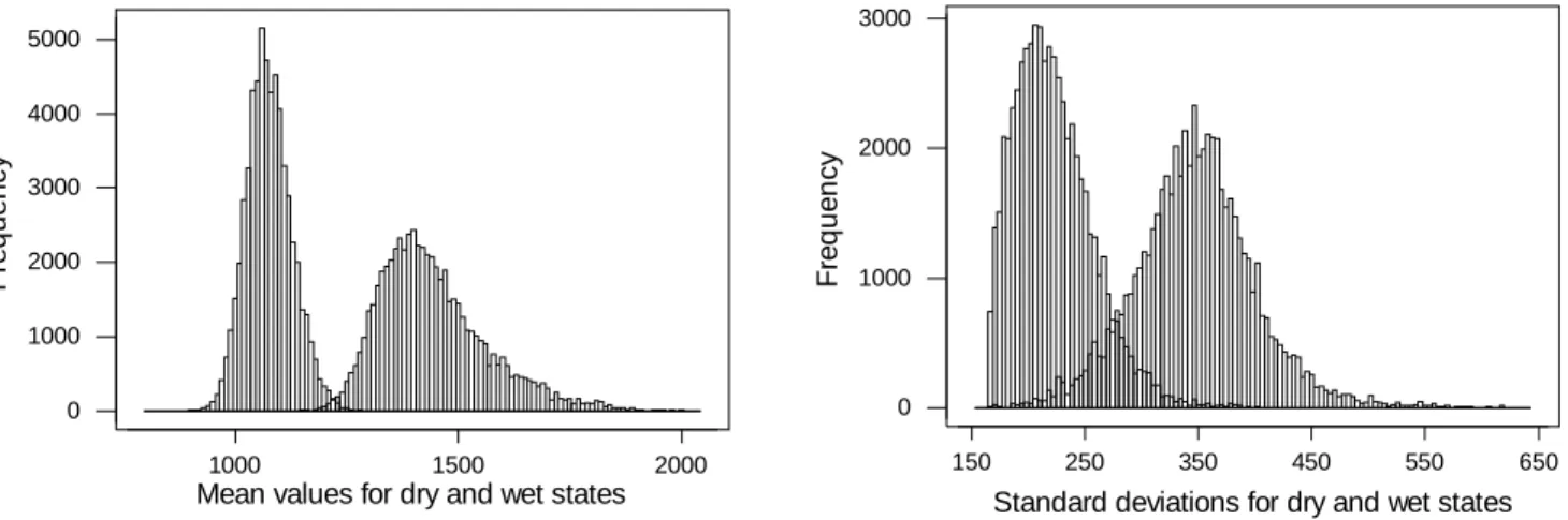
Although Markov processes are used to simulate the data set, the Markov chain is not observed directly, instead being hidden within an observation process that is a noisy function of the chain (Elliot et al., 1995). The two states are assumed to be independent Gaussian distributions, which requires six parameters to be defined – the mean m and variance s2 of each state and two transition probabilities P(W→D) and P(D→W). The probability that the simulated data remains in the same state for consecutive sampling periods is found as the complement of the respective transition probability. The histogram of the annual Sydney rainfall is shown in Fig. 7, and it is assumed that this distribution separates into twostate distributions in the HSM structure. Markov Chain Monte Carlo (MCMC) simulation techniques are used to determine the posterior distributions for the model parameters, the posterior distribution of estimates for the mean and standard deviation of each state being shown in Fig. 8.
Figure 8 suggests that a two-state HSM model could be a suitable representation of the annual rainfall time series of Sydney. The posterior distributions of the mean rainfall in the two states separate well in Fig. 8a, suggesting that annual rainfall has means of 1444 mm and 1076 mm within the two climate states, with the two standard deviations estimated from Fig. 8b as approximately 327 mm and 222 mm for the wet and dry states respectively. The posterior distributions for the estimates of the two transition probabilities in Fig. 9 are more dispersed than either the means or standard deviations, evidence that the HSM model is unable to make a strong estimate of these probabilities. The posterior for P(W→D) has a mean 0.420 and standard deviation 0.198, with P(D→W) having a mean 0.306 and standard deviation 0.148.
From the application of the two-state HSM model to the annual rainfall time series for Sydney, the posterior probability of a year existing in either climate state can be 5 4 3 2 3 2 1 ln(m) ln (R m )
Fig.6. Rescaled adjusted range for the time series of annual rainfall on Sydney (1859 – 1999). Slope of regression line, H = 0.76
203 2500 1500 500 25 20 15 10 5 0 Annual rainfall (mm) F re que nc y
Fig. 7. Histogram of annual rainfall in Sydney (1859–1999)
650 550 450 350 250 150 3000 2000 1000 0
Standard deviations for dry and wet states
F re que nc y 2000 1500 1000 5000 4000 3000 2000 1000 0
Mean values for dry and wet states
Fr
e
q
ue
ncy
Fig. 8. Posterior distributions of the two-state means (a) and two-state standard deviations (b) for annual rainfall
Fig. 9. Posterior distributions of the two HSM transition probabilities, P (W D) (a) and P (D W) (b)
1.0 0.5 0.0 1000 500 0 P(Wet to Dry) F re q ue nc y 1.0 0.5 0.0 2000 1000 0 P(Dry to Wet) F re q ue nc y
calculated by using the Baum–Welch forwards and backwards recursion (see Bengio, 1999). From this algorithm, the probability of the climate in year t existing in a “wet” state, conditional upon the entire rainfall series, P (st=W | Y1T) is calculated for the length of the annual rainfall
time series, with the results shown in Fig. 10.
From Fig. 10, the period 1905–1945, which was identified as being a ‘dry’ epoch in the time series of Fig. 2a, has a mean value of 0.37 for P (st=W | Y1T), which is lower than
the mean of 0.59 from across the entire time series. This suggests that the HSM model is able to model this period as predominantly a ‘dry’ state.
By using the mean values of the posterior distributions of HSM model parameters to simulate 1000 separate HSM chains, the behaviour of the Hurst coefficient can be
obtained. This Monte Carlo process displays a mean Hurst coefficient of 0.596, with 5% and 95% quantiles of 0.44 and 0.77 respectively. This interval just includes the value of the Hurst coefficient for the Sydney rainfall, 0.76. HSM MODELS AS MIXTURE MODELS
A mixture of two normal distributions can often closely approximate a skewed distribution. An HSM model includes a mixture as the special case of state transitions that are independent of the current state. In this special case, there is no persistence in states. Let PD and PW be the proportion of dry and wet states respectively. Then
1
P
P
D+
W=
(7a)Define PWD as P(W→D) , and similarly for the other transition probabilities. If the HSM model is merely a mixture, W DW WW D DD WD P P P P P P = = = = (7b)
and it follows from (7a) that
1
P
P
WD+
DW=
(7c)If there is a tendency to persist in the states, the sum of PWD and PDW will be less than 1, whereas the sum being greater than 1 would correspond to a tendency to fluctuate between states.
Figure 11 shows the posterior distribution of the sum of the two transition probabilities for the two-state HSM model applied to the Sydney annual rainfall time series, which has a skewness of 0.6072. Dashed lines show the 5% and 95% quantiles for this estimate, which are at 0.336 and 1.143
respectively. As this interval includes 1, there is no evidence that the estimates of the HSM parameters are different from a mixture distribution at a 10% significance level.
However, Thyer and Kuczera (2000) found that the estimates of transition probabilities were sensitive to the definition of the water year, which are equated with the calendar year. There is some justification, based on climatic indices (as discussed later), to prefer an April to March water year for New South Wales. In this case, the 95% and 98% confidence intervals for (PWD + PDW) are [0.285, 0.976] and [0.196, 1.116] respectively.
Although a two-state HSM model shows potential as a method of reproducing the apparent persistence in the annual rainfall time series of Sydney, it might be claimed that the fitted model is merely a normal mixture.
1.0 0.9 0.8 0.7 0.6 0.5 0.4 0.3 0.2 0.1 0.0 1985 1960 1935 1910 1885 1860 P (s tat e= W e t | r a in fa ll)
Fig. 10. Posterior wet state series values for the HSM model fitted to
the annual Sydney rainfall
2 1 0 2000 1000 0
Sum of transition probabilities
Fre q u e n c y
Fig. 11. Posterior distribution of the sum of the two transition
probabilities
Fig. 12. Variation in Hurst coefficient with variation in
autocorrelation from Monte Carlo simulations of AR (1) models, showing median and 95% and 5% quantiles
205 The cumulative sums provide evidence of non-stationarity.
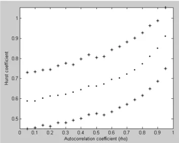
The Hurst coefficient provides some evidence that the rainfall time series is persistent, but this is not supported by the correlogram, or spectrum. It is worth noting that realisations of AR(1) series, which do not satisfy the mathematical definition of persistence, also exhibit Hurst coefficients that exceed 0.5, as shown in Fig. 12. In this figure, estimates for H from 1000 simulations each of length 100 are determined over a range of autocorrelation coefficients. From Fig. 12, the average value of the estimator of H in samples of discrete white noise of length 100 is 0.58. This bias reduces as the length of the time series increases.
Rainfall and climate interactions
RELATIONSHIPS WITH CLIMATE
The climate indices SOI, NINO3, IPO and PDO are related to rainfall across Australia. Their influence upon selected point rainfall can be investigated through observing correlations at annual scales, as shown in Table 4, where 5% significance is shown in italics. Annual values for each climate index are attained from the average of the January
0 500 1000 1500 2000 2500 1900 1910 1920 1930 1940 1950 1960 1970 1980 1990 S y d n ey a n n u al r a in fa ll ( m m ) -2.5 -2 -1.5 -1 -0.5 0 0.5 1 1.5 2 2.5 P D O i n d e x (m ul ti pl ie d by -1 ) 0 500 1000 1500 2000 2500 1900 1910 1920 1930 1940 1950 1960 1970 1980 1990 S y d n ey a n n u al r a in fa ll ( m m ) -25 -20 -15 -10 -5 0 5 10 15 20 25 An n u a l S O I
to December monthly totals for each year. Continuous data sets for SOI are available from 1876-2001, NINO3 from 1856–2000, IPO from 1857–1999 (data set from Folland et al., 1998) and PDO from 1900-2000.
If variables are correlated, averaging tends to give higher correlation. This accounts for the regional rainfall statistics having higher correlations to climate indices than point rainfall. By aggregating rainfall over the 107 Australian rainfall districts and distributing this into four regions across the continent, Simmonds and Hope (1997) showed that annual rainfall across New South Wales and Victoria had a correlation of 0.58 with annual SOI for the period 1913–1991. Regression analyses of point rainfall at Sydney (yt) on
Fig. 12. Time series of annual rainfall Sydney rainfall (solid line), annual PDO index and annual SOI (both dotted lines)
Location SOI NINO3 PDO IPO
Sydney 0.279 -0.211 -0.314 -0.239
Brisbane 0.423 -0.417 -0.281 -0.275
Melbourne 0.201 -0.277 -0.149 -0.156
Perth 0.294 -0.201 -0.087 0.038
Table 4. Correlations between annual totals of rainfall and climate
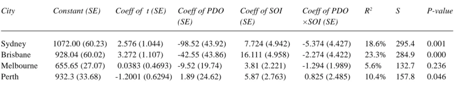
Table 5. Coefficients and standard errors for regression of annual rainfall for four capitals against climate indices, with R2 values,
standard deviation of residuals and overall P-value.
City Constant (SE) Coeff of t (SE) Coeff of PDO Coeff of SOI Coeff of PDO R2 S P-value
(SE) (SE) ×SOI (SE)
Sydney 1072.00 (60.23) 2.576 (1.044) -98.52 (43.92) 7.724 (4.942) -5.374 (4.427) 18.6% 295.4 0.001
Brisbane 928.04 (60.02) 3.272 (1.107) -42.55 (43.86) 16.111 (4.958) -2.274 (4.422) 23.3% 284.9 0.000
Melbourne 655.65 (27.07) 0.0383 (0.4693) -9.52 (19.74) 3.81 (2.221) -1.294 (1.989) 5.6% 132.7 0.236
Perth 932.3 (33.68) -1.2001 (0.6294) 1.89 (24.62) 5.87 (2.763) 0.825 (2.485) 10.4% 157.8 0.046
SOI, PDO and NINO3 and all their possible interactions, together with time, led to the following equation which had the smallest estimated standard deviation of errors:
( 37 . 5 SOI 72 . 7 PDO 98.5 t 2.58 1072 yt = − × − × + × − × (8) where t is the time in years from the beginning of the record. This equation is statistically significant (P≈0.001). Although the PDO is the most statistically significant predictor variable, this regression is better than a regression of only the PDO index against the annual rainfall in Sydney inasmuch as the standard deviation of the residual errors was reduced from 305.9 to 295.4.
Table 5 shows the coefficients (with standard errors) for regression models of each of the four capital cities against the predictor variables used in Eqn. (6).
The influence of these regression variables on rainfall in Australia supports the work of various authors (e.g. Power et al., 1999) who have shown inter-relationships between changes in the SOI, Australian climate variables and the inter-decadal SST modulation in the Pacific, identified by the PDO index. By including PDO in the regression of the annual rainfall of Sydney on SOI, a better fit was achieved, suggesting that similar relationships are still statistically significant when observing only point rainfall.
Figure 12 compares the time series of annual rainfall in Sydney with annual values of the SOI and PDO index, multiplied by minus one, over the period 1900–1999.
The correlations between the time series of Fig. 12 are shown in Table 6, with P-values shown in brackets. The five-year variance of the annual rainfall series was calculated over consecutive five-year periods, centred at 1900, 1905, etc. and this series is also correlated to the climate indices and shown in Table 6.
Table 6 indicates that not only is the annual rainfall of Sydney significantly correlated with the PDO index, but so is the variability in the annual rainfall. Although the SOI is also significantly correlated with the annual rainfall, it does
not show evidence of being significantly related to the variance in the annual rainfall time series. Regression analysis of the log transform of the five-year variance in the mean annual rainfall on PDO and time (t) yields the following equation:
1n (Five year variance of yt) = 10.7 + 0.0299 × t – 0.420 × PDO (9) which is statistically significant (P≈0.038). The inclusion of SOI and the interaction between PDO and SOI did not improve the regression model of variances in yt.
The significant correlations between the mean annual rainfall in Sydney and climate indices suggests that long-term simulation of rainfall would be improved when including the role of the climate indices. A regression model of the mean annual rainfall of Sydney on time, the SOI, PDO index and their interaction is a possible method of long-term simulation. Such simulation requires the development of forecast models for the two climate indices, together with a suitable model for residuals.
FITTING MODELS TO SOI AND PDO INDICES Forecast models for the annual SOI and PDO indices over the period 1900–1999 require the investigation of both the short and long-term persistence behaviour of these time series. The correlograms for these indices are displayed in Figs. 13 and 14. There is no suggestion of autocorrelation Table 6. Performance of the regression model in equation 10 for
the simulation of annual Sydney rainfall (1900-1999) over 10000 simulations, with mean and 5% and 95% quantiles provided
Variable Annual PDO Annual SOI
index
Sydney annual rainfall -0.314 (0.001) 0.253 (0.011)
Five year variances of rainfall -0.322 (0.001) -0.005 (0.961)
SOI) (PDO×
207 in the SOI, but the PDO index has substantial
autocorrelations up to lag 7.
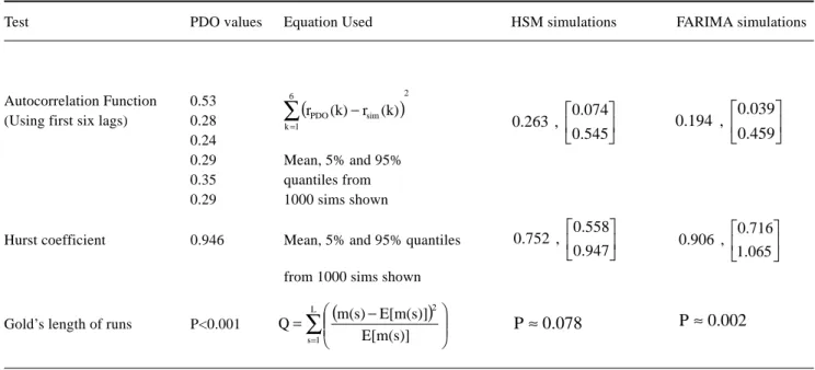
The Hurst coefficients are 0.668 for the SOI and 0.946 for the PDO respectively. There is evidence to reject the null hypothesis that the PDO index is a realisation of independent variables. The fractional ARIMA (0, d, 0) model had a lower AIC value than either the AR(1) model, or a MA(7) model, which is suggested by Fig. 14. Furthermore, the FARIMA(0, d, 0) model is capable of simulating the high Hurst coefficient of the annual PDO index.
A two-state HSM model is an alternative to a FARIMA(0, d, 0) model for simulating annual totals of the PDO index. After applying a two-state HSM model to annual values of the PDO index for the period 1900–1999, Figs. 15 and 16 show the posterior distributions for the two state means and the sum of the two transition probabilities. Figure 16 suggests that the HSM model can successfully identify two states in the annual data, with means for the two state posteriors of 0.4082 and –0.6157. The posterior distribution of the sum of the two transition probabilities has a mean of 0.200 and a standard deviation of 0.092, providing strong evidence for persistence rather than a mixture.
Table 7 shows a comparison between the performance of a two-state HSM model and a FARIMA(0,d,0) to simulate annual totals of the PDO index. Three diagnostic tests have been used to compare the performance of these two processes. The autocorrelation function and the Hurst
Table 7. Comparison of the performance of HSM and FARIMA(0,d,0) models for the simulation of the annual
PDO index (1900–1999)
Test PDO values Equation Used HSM simulations FARIMA simulations
Autocorrelation Function 0.53
(Using first six lags) 0.28
0.24
0.29 Mean, 5% and 95%
0.35 quantiles from
0.29 1000 sims shown
Hurst coefficient 0.946 Mean, 5% and 95% quantiles
0.947 0.558 , 0.752 1.065 0.716 , 0.906
from 1000 sims shown
Gold’s length of runs P<0.001 P≈0.078 P≈0.002
coefficient for 1000 simulations of length 100 years, for each of these two models have been compared with the annual PDO index over the period 1900–1999. Thirdly, the length-of-runs test (see Srikanthan et al., 1983) has been used to compare the ability of both processes to simulate any “runs” (consecutive values either side of the mean) in the PDO time series. If m(s) denotes the total number of runs of length s above and below the median, then for a random process, the expected value of m(s) is:
1 s 2 / s] 3 [n E[m(s)]= + − + (10)
The sum Q shown in Table 7 is distributed as chi-square with (L-1) degrees of freedom, where L is the maximum run length. High values for Q are evidence that the sequence is a non-independent random variation. The results of diagnostic testing in Table 7 indicate that a FARIMA (0, 0.446, 0) model is superior to a two-state HSM model for the simulation of annual values for the PDO index over the period 1900–1999.
The SOI shows a statistically significant correlation of –0.492 with the annual PDO index over the period 1900-1999. A linear regression model is used to simulate the SOI, conditioned upon the PDO. The fitted model is
PDO 4.40 0.204
SOI= − × (11)
The standard error of the coefficient of PDO is 0.786. There is no evidence that the residuals are autocorrelated and they
(
)
2 6 1 k sim PDO(k) r (k) r∑
= − 0.459 0.039 , 0.194 0.545 0.074 , 0.263(
)
∑
= − = L 1 s 2 E[m(s)] E[m(s)] m(s) QFig. 13. Correlogram for annual SOI (1900 – 1999)
Fig. 14. Correlogram for annual PDO index (1900 – 1999)
24 14 4 1.0 0.8 0.6 0.4 0.2 0.0 -0.2 -0.4 -0.6 -0.8 -1.0 A u to c o rr el at io n 24 14 4 1.0 0.8 0.6 0.4 0.2 0.0 -0.2 -0.4 -0.6 -0.8 -1.0 A u to c o rr el at io n 1 0 -1 5000 4000 3000 2000 1000 0
mean values for dry and wet states
F
re
que
nc
y
Fig. 15. Posterior distribution of the two state means for annual
PDO index (1900 – 1999) 0.7 0.6 0.5 0.4 0.3 0.2 0.1 0.0 1500 1000 500 0
Sum of transition probabilities
F
re
que
nc
y
Fig. 16. Posterior distribution of the sum of the two transition
probabilities for annual PDO index (1900 – 1999)
are realistically modelled as Gaussian, with mean = 0 and standard deviation = 6.097.
SIMULATIONS FROM A REGRESSION MODEL In a regression model for the long-term simulation of annual Sydney rainfall, a log transform of the annual rainfall data was used to obtain residuals that were approximately Gaussian (Anderson-Darling statistic = 0.246 compared with 1.001 for untransformed data). Furthermore, regression of the logarithm of the 5-year variances of the log-transform of the rainfall was not statistically significant. The correlogram of these residuals is shown in Fig. 17, and is consistent with independence. Residuals have a Hurst coefficient of 0.53, which suggests that there is no long-term dependence in the time series of residuals. Any persistence in the annual Sydney rainfall (yt) is expected to arise from conditioning on the PDO index.
It should be noted that cross-correlation between a stochastic process (Yt) and a persistent stochastic process (Xt) does not imply Yt must itself be persistent. This follows from the fact that a persistent stochastic process can be constructed from a sum of AR(1) processes if the parameters
α have an approximate beta distribution (Beran, 1994).
A set of 10000 simulations of yt were calculated using the regression model:
t) 6.96 0.002 t -0.077 PDO 0.00638 S
ln(y = + × × + ×
(12) where εt are Gaussian residuals, mean = 0 and standard deviation = 0.2433.
The performance of this model over 10 000 simulations of length 100 is outlined in Table 8, in which the mean, 5% and 95% quantiles are provided for the three time series characteristics: mean, standard deviation and Hurst coefficient. The results shown in Table 8 indicate that the simulation model is capable of reproducing important characteristics of the annual rainfall time series from Sydney, including its persistence. Figure 18, which is a probability plot of yt with 5% and 95% bounds determined from the
25 15 5 1.0 0.8 0.6 0.4 0.2 0.0 -0.2 -0.4 -0.6 -0.8 -1.0 A u to c o rr el at io n
Autocorrelation Function for regression residuals
Fig. 17. Correlogram for residuals from simulation model
t SOI) (PDO 0.0032 -SOI × × +ε
209 Table 8. Performance of the regression model in Eqn.(10) for the
simulation of annual Sydney rainfall over 10 000 simulations, with mean and 5% and 95% quantiles provided.
Characteristic Annual Sydney Regression model rainfall simulations (1900-1999)
Mean 1211.6 1250.9 [1152.6, 1434.2]
Standard Deviation 320.6 324.8 [267.9, 407.9]
Hurst Coefficient 0.781 0.683 [0.527, 0.837]
10000 simulations shown either side of the yt, gives a further indication of the ability of the simulation model to reproduce the structure of the rainfall time series.
Table 9a gives the regression of the log-transform of the rainfall against PDO, SOI and their interaction for all four state capitals. The standard errors of the coefficients are
500 1000 1500 2000 2500 3000 .01 .1 1 5 10 20 30 50 70 80 90 95 99 99.9 99.99 A n nual r a in fa ll ( m m ) Percent
Fig. 18. Probability plot for annual Sydney rainfall (1900-1999),
with 5% and 95% confidence bounds estimated from Monte Carlo simulation
Table 9(a) Coefficients and standard errors for regressions of log transform of annual rainfall (January–December) in
four capitals against climate indices, with R2 values, standard deviation of residuals and overall P-value
City Constant (SE) Coeff of t Coeff of PDO Coeff of SOI Coeff of PDO R2 S P-value
(SE) (SE) (SE) ×SOI (SE)
Sydney 6.960 0.0020 -0.077 0.0064 -0.0032 16.9% 0.2433 0.001 (0.050) (0.0009) (0.036) (0.0041) (0.0036) Brisbane 6.798 0.0030 -0.049 0.015 -0.0026 22.7% 0.2752 0.000 (0.058) (0.0011) (0.042) (0.005) (0.0043) Melbourne 6.467 0.0000 -0.015 0.0061 -0.0018 5.6% 0.2111 0.241 (0.043) (0.0007) (0.031) (0.0035) (0.0032) Perth 6.820 -0.0013 0.0033 0.0075 0.0014 10.9% 0.1865 0.038 (0.040) (0.0007) (0.0291) (0.0033) (0.0029)
Table 9(b) Coefficients and standard errors for regressions of log transform of annual rainfall (April–March) in four capitals against
climate indices, with R2 values, standard deviation of residuals and overall P-value
City Constant (SE) Coeff of t Coeff of PDO Coeff of SOI Coeff of PDO R2 S P-value
(SE) (SE) (SE) ×SOI (SE)
Sydney 6.947 0.0022 -0.0555 0.0061 -0.0065 16.3% 0.2389 0.002 (0.049) (0.0009) (0.0357) (0.0040) (0.0036) Brisbane 6.822 0.0025 -0.0751 0.0053 -0.0033 12.5% 0.300 0.018 (0.064) (0.0012) (0.0467) (0.0053) (0.0047) Melbourne 6.4525 0.0002 -0.0036 0.0071 -0.0040 8.2% 0.1934 0.088 (0.040) (0.0007) (0.0289) (0.0032) (0.0029) Perth 6.823 -0.0015 0.0208 0.0100 -0.0003 16.6% 0.1733 0.003 (0.037) (0.0007) (0.0272) (0.0031) (0.0027)
given in brackets. Allan et al. (1996) indicated that significant changes in climatic indices tend to occur in the Austral autumn. This suggests that using water years of April to March may be more informative as there will be less averaging out of any change in such indices over a year. Table 9b gives the corresponding regressions.
Conclusions
A 40-year ‘dry’ period in the time series of annual Sydney rainfall is apparent in the time series plot and the ending of this period has been shown to correspond to an increase in flood risk in New South Wales. This non-stationarity was formally demonstrated to be statistically significant by CUSUM analysis. Although this phenomenon might reasonably be described as persistence, the correlogram and spectrum provide no evidence for the mathematical persistence that is so noticeable in the time series of Nile River flows. The Hurst coefficient however is higher than expected for a realisation of independent variables, suggesting that a two-state HSM model might be appropriate.
HSM models provide a good fit to the annual Sydney rainfall data but the evidence that this is anything more than a mixture of normals well approximating a skewed distribution is not overwhelming and depends on the definition of water year.
Various climate indices, including the SOI, NINO3 and the PDO index are related to rainfall across Australia. Regressions of the annual point rainfall in Sydney, Brisbane and Perth on the time since the start of their records, found that the SOI, the PDO index and their interaction were all statistically significant. The influence of both the SOI and the PDO index on the annual point rainfall records supports the views of other authors (eg Power et al., 1999) who have identified inter-relationships between changes in the SOI, rainfall in Australia and changes in Pacific SSTs.
A regression of the log-transform of the rainfall series on the same predictor variables was used for the long-term simulation of annual Sydney rainfall. By simulating annual values of the PDO index with a FARIMA(0,d,0) model and the SOI from a linear relationship with the PDO, a suitable simulation model was established. Statistical characteristics such as the mean and standard deviation of simulated time series were significantly close to those of the Sydney rainfall, together with persistence identified by the Hurst coefficient. Similar models were formulated for the other capital cities. The standard deviation of rainfall was also related to the PDO index.
Power et al. (1999) distinguished thresholds of –0.5 and 0.5 in the monthly IPO time series as marking significant
changes in the relationships between the IPO index and Australian rainfall. Correlations between all-Australian averaged rainfall and the IPO were identified by Power et al. (1999) as being significantly higher for months in which the IPO were less than –0.5. Although monthly rainfall regressions for Sydney were more significant for certain months (i.e. January, February, June, July, November), no evidence of a similar threshold was observed in the annual point rainfall series.
Acknowledgements
The authors wish to thank Assoc. Prof. George Kuczera and Dr. Stewart Franks from the University of Newcastle for valuable discussions and their thoughts concerning the direction of this work.
References
Allan, R.J., Lindesay, J.A. and Parker, D., 1996. El Nino Southern
Oscillation and Climatic Variability. Collingwood, Australia,
CSIRO Publishing.
Bengio, Y., 1999. Markovian Models for Sequential Data. Neural
Computing Surveys 2, 129–162.
Beran, J., 1994. Statistics for Long-Memory Processes. Chapman and Hall, New York.
Chiew, F.H.S. and McMahon, T.A., 2003. El Nino/ Southern Oscillation and Australian rainfall and streamflow. Austral. J.
Water Resour., 6, 115–129.
Chiew, F. H. S., Piechota, T.C., Dracup, J.A. and McMahon, T.A., 1998. El Nino/Southern Oscillation and Australian rainfall, streamflow and drought: Links and potential for forecasting. J.
Hydrol., 204, 138–149.
Cornish, P.M., 1977. Changes in Seasonal and Annual Rainfall in New South Wales. Search 8, 38–40.
Elliott, R.J., Aggoun, L. and Moore, J.B., 1995. Hidden Markov
models: estimation and control. Springer, New York.
Folland, C.K., Parker, D.E., Colman, A.W. and Washington, R., 1998. Large-scale modes of ocean surface temperature since the late nineteenth century. Rept. No. CRTN81, UK Meteorolgical Office.
Franks, S.W., 2002. Assessing hydrological change: deterministic general circulation models or spurious solar correlation? Hydrol.
Process., 16, 559–564.
Harrsion, S.P. and Dodson, J.,1993. Climates of Australia and New Guinea since 18,000 yr B.P. In: Global Climates since the Last
Glacial Maximum, H.E. Wright Jr., J.E. Kutzbacj, T. Webb III,
W.F. Ruddimann, F.A. Street-Perrott and P.J. Bartlein (Eds.) University of Minnesota Press, Minneapolis, USA. 265–293. Hosking, J.R.M., 1984. Modelling Persistence in Hydrological
Time Series Using Fractional Differencing. Water Resour. Res., 20, 1898–1908.
Hurst, H.E., 1951. Long-term storage capacity of reservoirs. Trans.
Amer. Soc. Civ. Engrs, 116, 770–799.
Latif, M., Kleeman, R. and Eckert, C., 1997. Greenhouse Warming, Decadal Variability, or El Nino? An Attempt to Understand the Anomalous 1990s. J. Climate, 10, 2221–2239.
Mantua, N., Hare, S.R., Zhang, Y., Wallace, J.M. and Francis, R.C., 1997. A Pacific interdecadal climate oscillation with impacts on salmon production. Bull. Amer. Meteorol. Soc., 78, 1069–1079.
211 McBride, J.L. and Nicholls, N., 1983. Seasonal Relationships
between Australian Rainfall and the Southern Oscillation. Mon.
Weather Rev., 111, 1998–2004.
Montgomery, D.C., 1991. Introduction to statistical quality
control. Wiley, New York.
Power, S., Casey, T., Folland, C., Colman, A. and Mehta, V., 1999. Inter-decadal modulation of the impact of ENSO on Australia.
Climate Dynamics 15, 319–324.
Simmonds, I. and Hope, P., 1997. Persistence Characteristics of Australian Rainfall Anomalies. Int. J. Climatol., 17, 597–613. Srikanthan, R., McMahon, T.A. and Irish, J.L., 1983. Time Series Analysis of Annual Flows of Australian Streams. J. Hydrol., 66, 213–226.
Thyer, M.A. and Kuczera, G.A., 2000. Modelling long-term persistence in hydroclimatic time series using a hidden state Markov model. Water Resour. Res., 36, 3301–3310.
Zhang, Y., Wallace, J.M. and Battisti, D.S., 1997. ENSO-like Interdecadal Variability: 1900-93. J. Climate, 10, 1004–1020.