HAL Id: hal-00317999
https://hal.archives-ouvertes.fr/hal-00317999
Submitted on 19 May 2006
HAL is a multi-disciplinary open access
archive for the deposit and dissemination of
sci-entific research documents, whether they are
pub-lished or not. The documents may come from
teaching and research institutions in France or
abroad, or from public or private research centers.
L’archive ouverte pluridisciplinaire HAL, est
destinée au dépôt et à la diffusion de documents
scientifiques de niveau recherche, publiés ou non,
émanant des établissements d’enseignement et de
recherche français ou étrangers, des laboratoires
publics ou privés.
ion acoustic speed?
M. V. Uspensky, A. V. Koustov, S. Nozawa
To cite this version:
M. V. Uspensky, A. V. Koustov, S. Nozawa. STARE velocity at large flow angles: is it related to the
ion acoustic speed?. Annales Geophysicae, European Geosciences Union, 2006, 24 (3), pp.873-885.
�hal-00317999�
www.ann-geophys.net/24/873/2006/ © European Geosciences Union 2006
Annales
Geophysicae
STARE velocity at large flow angles: is it related to the ion acoustic
speed?
M. V. Uspensky1, A. V. Koustov2, and S. Nozawa3
1Finnish Meteorological Institute, Erik Palminin Aukio 1, P.O. Box 503, Helsinki FIN-00101, Finland
2Institute of Space and Atmospheric Studies, University of Saskatchewan, 116 Science Place, Saskatoon, S7N 5E2, Canada 3Solar-Terrestrial Environment Laboratory, Nagoya University, Chikusa-ku, Nagoya 464-01, Japan
Received: 3 December 2005 – Revised: 15 February 2006 – Accepted: 8 March 2006 – Published: 19 May 2006
Abstract. The electron drift and ion-acoustic speed in the
E region inferred from EISCAT measurements are compared with concurrent STARE radar velocity data to investigate a recent hypothesis by Bahcivan et al. (2005), that the elec-trojet irregularity velocity at large flow angles is simply the product of the ion-acoustic speed and the cosine of an an-gle between the electron flow and the irregularity propaga-tion direcpropaga-tion. About 3 000 measurements for flow angles of 50◦–70◦and electron drifts of 400–1500 m/s are considered. It is shown that the correlation coefficient and the slope of the best linear fit line between the predicted STARE velocity (based solely on EISCAT data and the hypothesis of Bahci-van et al. (2005)) and the measured one are both of the order of ∼0.4. Velocity predictions are somewhat better if one as-sumes that the irregularity phase velocity is the line-of-sight component of the E×B drift scaled down by a factor ∼0.6 due to off-orthogonality of irregularity propagation (nonzero effective aspect angles of STARE observations).
Keywords. Ionosphere (Auroral ionosphere; Ionospheric
ir-regularities; Plasma waves and instabilities)
1 Introduction
Excitation of meter-scale electrojet irregularities is a well-known high-latitude phenomenon (e.g. Fejer and Kelley, 1980). The irregularity properties and mechanisms of their generation have been extensively studied with coher-ent radars and direct rocket measuremcoher-ents. It is now ac-cepted that the auroral electrojet irregularities are produced through the combined effect of the Farley-Buneman (FB) and gradient-drift (GD) plasma instabilities. Both theory and ex-periment convincingly show that many clues to the nature of electrojet irregularities can be obtained by studying the Correspondence to: A. V. Koustov
irregularity phase velocity variation with the flow angle, the angle of irregularity propagation with respect to the E×B electron flow at the E region heights.
For relatively fast flows, two ranges of flow angles, θ , are traditionally distinguished, inside and outside of the FB in-stability cone, corresponding to the regions of linearly un-stable and decaying waves, respectively. The numeric value for the FB cone angle, θ∗, is estimated from the condition cos θ∗=CS/VE×B, where CS the ion-acoustic speed of the
media and VE×B is the magnitude of the E×B electron flow
velocity. For typical conditions in the auroral ionosphere at 100–120 km, θ∗ is of the order of 40◦ and increases up to
∼70◦with the electron flow velocity. Outside the FB insta-bility cone, θ >θ∗, it is thought (e.g. Nielsen and Schlegel,
1985; Nielsen et al., 2002) that the irregularity phase veloc-ity can be described by equation
Vph=VE×B·cos θ , (1)
which is consistent with the linear theory of the FB and GD instabilities in its simplest form (Fejer and Kelley, 1980). Equation (1) implies that the irregularity velocity in a cer-tain direction is a cosine component of the E×B drift. This contrasts strongly with the situation within the FB instabil-ity cone, θ <θ∗, where the irregularity phase velocity is be-lieved to be independent of θ and close to CS (e.g. Nielsen
and Schlegel, 1985). A number of nonlinear theories support this notion (e.g. Fejer and Kelley, 1980; Schlegel, 1996; Sahr and Fejer, 1996).
The above understanding is supported by a number of coherent radar experiments (such as STARE and others) in which the echo velocity was compared with independent data on the plasma flow and ion-acoustic speed provided by con-currently operating incoherent scatter radars (e.g. Nielsen and Schlegel, 1985; Farley and Providakes, 1989; Kofman and Nielsen, 1990; Haldoupis and Schlegel, 1990; Chen et al., 1995; Foster and Erickson, 2000). The coherent radar line-of-sight (l-o-s) velocity is the irregularity velocity in
a single flow direction, and the irregularity velocity varia-tion with the flow angle can be studied by combining l-o-s measurements for various electrojet directions. Such joint STARE and EISCAT observations, performed more recently, showed significant departures from the above “expected” picture, both at small and large flow angles. At large θ , Kustov and Haldoupis (1992), Kohl et al. (1992), Koustov et al. (2002) and Uspensky et al. (2004) presented data in-dicating that the STARE radar velocity is typically smaller than the E×B electron flow component along the radar beam (velocity is “depressed”). For the STARE radars, the ratio of the observed velocity Vr to the electron flow component D=Vr/(VE×B·cos θ ) was found to be in the range of 0.3–
0.7. The most extended data set considered by Uspensky et al. (2004) indicates that D ∼0.55.
The effect of the velocity “depression” was attributed to nonzero effective aspect angles of observations, due to echo reception from a range of electrojet heights (Uspensky, 1985; Kustov and Haldoupis, 1992; Koustov et al., 2002; Uspensky et al., 2004). Kustov and Haldoupis (1992) assumed that the irregularity phase velocity follows the linear fluid theory of the FB and GD instabilities that allows irregularity propaga-tion not exactly perpendicular to the magnetic field:
Vph= 1
1 + RVE×Bcos θ = βVE×Bcos θ ;
R = νeνi ei(1 + 2e ν2 e sin2ψ ), (2)
where νe,i and e,i are the electron and ion collision
fre-quencies with neutrals and the gyrofrefre-quencies and ψ is the off-orthogonality angle (aspect angle in coherent radar obser-vations). Coefficient proportionality β depends strongly on
R. For very small off-orthogonality angles R is small (R 1) and β is close to 1. However, in the case of echo reception from a range of electrojet heights (a range of nonzero aspect angles), R can be comparable or even larger than 1.
Later HF radar observations by Uspensky et al. (2001) along the flow and by Makarevitch et al. (2002) and Uspen-sky et al. (2003) at θ ∼90◦ (at HF and VHF, respectively) suggested that the ion contribution to the irregularity phase velocity can be important. According to the linear theory of the electrojet instabilities with the ion motion taken into ac-count
Vph=βVE×Bcos θ + R
1 + RV0icos 8, (3)
where V0iis the velocity of the ion drift and 8 is the angle be-tween the irregularity propagation direction and the ion drift vector. Unless the angle θ is close to 90◦and R>1, the sec-ond term in Eq. (3) is negligible. The important role of the ion motion term was elucidated by Uspensky et al. (2003) who presented a short example of measurements for which the STARE Finland velocity was almost two times larger than the one expected from Eq. (1) and certainly from Eq. (2). The authors termed the effect “the velocity overspeed”, which
seemed to be strange and inconsistent with the velocity de-pression phenomenon, but the authors discovered that the ef-fect was observed for the periods of very low density in the E region, so that echoes were very likely received from only large heights where the ion motion contribution to the irreg-ularity phase velocity could indeed be expected. Another ex-pectation from Eq. (3) is that at θ ∼90◦the phase velocity can be close to the l-o-s component of the ion drift. Recently, Makarevich et al. (2005)1 investigated this expectation by comparing the STARE Finland velocity and the E-region ion drift measured directly by EISCAT. A reasonable agreement between the two was found.
For observations within the FB instability cone, the un-derstanding has been evolving as well. First, it was discov-ered that the STARE Doppler velocity can be above CS
(Kof-man and Nielsen, 1990; Haldoupis and Schlegel, 1990) and it changes with the flow angle (Chen et al., 1995). A more systematic study of both effects has been recently performed by Nielsen et al. (2002). These authors reported that, along the electron flow direction, the ratio of the l-o-s velocity Vr
and CS can be as large as 1.2, and the velocity variation with
the flow angle can be described by
Vr =mαCScosαθ, (4)
where the coefficient of proportionality m is of the order of 1.3 and the value of α changes from 0.8 to 0.2 as the electron drift increases from 600 to 1600 m/s. Nielsen et al. (2002) concluded that only at flow angles of ∼40◦(typical angles
θ∗)the irregularity phase velocity is close to CSand Eqs. (1)
and (4) produce the same result. According to Nielsen et al. (2002), well outside the FB cone, the irregularity phase velocity follows Eq. (1), though it should be commented that the data statistics at these flow angles was insignificant in this study.
Recently, Bahcivan et al. (2005) proposed a new scenario on the irregularity velocity change with the flow angle. They suggested that the FB irregularities move with the velocity close to CSonly at very small flow angles, mostly along the
electron flow direction. For all other directions, including
θ >θ∗, the velocity variation follows
Vph=CScos θ. (5)
Equation (5) is similar to Eq. (1), except that the coefficient proportionality in front of the cosine function is CS and not VE×B. In this ideology, the cone angle θ∗ does not have any special meaning. To support this hypothesis, Bahcivan et al. (2005) first presented 30-MHz radar velocities (5-m elec-trojet irregularities) and concurrent electron drifts measured (for θ =50◦–60◦)on board of two rocket flights in Alaska.
The CS values were estimated by using results of previous
1Makarevich, R. A., Honary, F., Howells, V. S. C., Koustov, A.
V., Milan, S. E. Davies, J. A., Senior, A., McCrea, I. W., and Dyson, P. L.: A first comparison of irregularity and ion drift velocity mea-surements in the E region, Ann. Geophys., submitted, 2005.
publications. The authors then investigated the STARE data published by Uspensky et al. (2004). In both cases, it was found that Eq. (5) works reasonable well.
Hypothesis (5) gives theorists a hint on a new physics of irregularity formation, especially outside the FB instability cone, as it relates the irregularity velocity not so much with the electron drift as with the ion-acoustic speed. It is thus fundamentally important to know whether this idea, so far based on a very limited data set, is generally correct. For brevity, we shall call predictions based on Eq. (5) “the CS
model”.
The purpose of this study is to make a more comprehen-sive assessment of the suggestion of Bahcivan et al. (2005) by, first, thoroughly reprocessing the data studied by Uspen-sky et al. (2004) and second, by involving a much more sig-nificant data set.
2 Quantitative analysis of the 12 February 1999 event
In their study, Bahcivan et al. (2005) scaled data from the diagrams published by Uspensky et al. (2004) for the Nor-way radar and analyzed them. It is important to know that the data of Uspensky et al.’s (2004) were smoothed for the purpose of presentation, and this can introduce some error in their assessment. Here we perform more rigorous analysis by working with the original data for both the Norway and Finland radars.
For the reader’s convenience, one is reminded that be-tween 11:00 UT and 16:00 UT on 12 February 1999, both STARE radars were operated simultaneously with the EIS-CAT UHF radar working in the CP 1 (field-aligned) mode. The 1-min EISCAT data on the electric field, and electron and ion temperatures were extracted. The values of the ion-acoustic speed CS were computed from the electron and
ion temperatures at 111 km, assuming the ion mass to be 30 a.m.u., and both electrons and ions are isothermal. The electron E×B velocity magnitude varied between 200 and 1500 m/s while the azimuth was close to the westward orien-tation.
The STARE radars were working in the usual mode, switching between the double-pulse (DP) and multi-pulse (MP) measurements of the velocity. One cycle of measure-ments lasted 20 s. In this section we consider DP velocity measurements for the Norway radar and MP data for the Fin-land radar to be consistent with Uspensky et al. (2004), who adopted the DP velocities for the Norway radar because the MP data were not as frequent as the DP data (due to several poor lags of the autocorrelation function). Later analysis by Uspensky et al. (2005) showed that the DP Norway veloci-ties are typically ∼1.1 times smaller than the MP velociveloci-ties, which is not a significant difference for the purposes of the present paper. For the Finland radar, the DP/MP velocity differences are significant, by a factor of 1.7, and we
con-sider only MP data for the Finland radar, similar to Uspensky et al. (2004).
In this study we had available 1-min EISCAT data and 20-s STARE data. To compare observations with such a different resolution, we decided to interpolate the EISCAT data to in-crease the statistics so that the joint data would be available every 20 s. In addition, for every STARE MP measurement we used data collected in 5 consecutive 20-s intervals, cen-tered around each 20-s interval, to operate with better STARE autocorrelation functions and decrease the clutter contamina-tion effects discussed by Uspensky et al. (2005).
2.1 CSmodel predictions for the height of 111 km
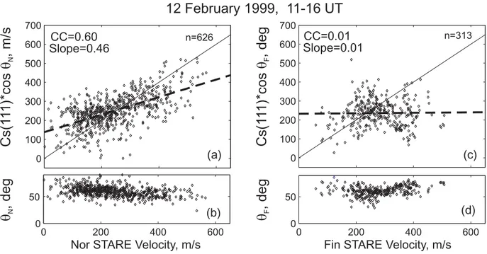
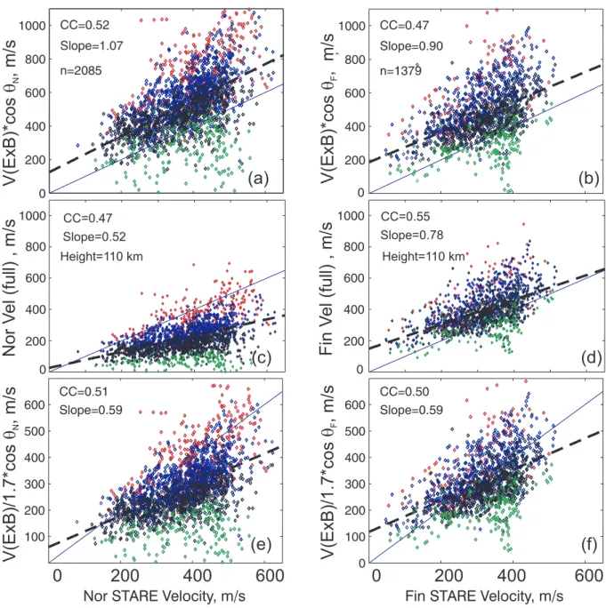
Figure 1 is a 4-panel diagram presenting data relevant to the Norway (left column) and Finland (right column) radars. Figures 1a, c are scatter plots of the irregularity phase veloc-ity predicted by the CSmodel (solely from the EISCAT data)
versus the measured velocity, for the Norway and Finland radars, respectively. Total number of points is given in the top right corner of each panel. Figures 1b, d show the flow angles of observations for each radar. In the left top corners of Figs. 1a, c we indicate the correlation coefficient (CC) be-tween the predicted irregularity velocity, and the measured velocity and the slope of the best linear fit line. The best fit lines are drawn by the dashed line across the cloud of points. The solid bisectors in Figs. 1a, c correspond to the case of ideal agreement between predictions and measurements.
We would like to point out that for both radars the flow angles were comparable, in the range of 50◦–70◦(c.f. data in Figs. 1b and d), with somewhat larger Finland flow angles. Comparing the spread of points in all the diagrams, one can conclude that the Norway data are better clustered than the Finland data. This fact is reflected in the better correlation coefficient for the Norway radar. In terms of velocity magni-tude, for the Norway radar (Fig. 1a), one can notice that the cloud of points is centered slightly above the bisector of ideal agreement at low measured velocities and below the bisector at large measured velocities, consistent with the fact that the slope of the best linear fit line is ∼0.5. For the Finland radar, Fig. 1c, the point clustering is poor, and the best fit line is al-most horizontal. There are points with reasonable agreement between predictions and measurements.
In summarizing the analysis of the 12 February 1999 event, one can conclude that the Finland radar data do not support the CS model of Bahcivan et al. (2005). The claim
of these authors on the agreement between the CSmodel
pre-dictions and the observations for the Norway radar data can only be accepted marginally.
2.2 CS model comparison for other possible heights of
backscatter
One can argue that the above analysis was performed by as-suming one echo height of 111 km. This choice might be not
0 100 200 300 400 500 600 700
CC=0.01
Slope=0.01
(d)
n=313 0 200 400 600 0 50 50Fin STARE Velocity, m/s
0 100 200 300 400 500 600 700
CC=0.60
Slope=0.46
(a)
(c)
12 February 1999, 11-16 UT
n=626 0 200 400 600 0Nor STARE Velocity, m/s
(d)
(b)
,
deg
q
NCs(1
1
1)*cos
,
m/s
q
N,
deg
q
FCs(1
1
1)*cos
,
deg
q
FFig. 1. (a) and (c): A comparison of the predicted and measured velocity for the Norway and Finland STARE observations over the EISCAT
spot for 12 February 1999. For predictions, the irregularity phase velocity was assumed to be the line-of-sight component of the ion-acoustic
speed CS at 111 km. Panels (b) and (d) present the flow angles of observations for the Norway and Finland radars, respectively. The
correlation coefficients and the slopes of the best linear fit line are given in the top left part of plots (a) and (c). The number n is the total number of points involved in respective comparison.
the best one as the zero rectilinear aspect angles of observa-tions are achieved at lower heights for both STARE radars (Koustov et al., 2002). Moreover, the height of STARE echoes was not measured in this experiment and generally it is not well known. For this reason, we assessed the CS
model predictions for the Norway radar and for CS values
at three potentially possible heights of 99 km, 105 km and 111 km (there is no point in assessing the Finland data as they simply do not support the model, Fig. 1c). We selected only those moments for which simultaneous data were avail-able at all three heights. Such a selection decreased the total amount of points available for each plot (e.g. compare with the number of points at 111 km in Fig. 1), but the selection of simultaneous data at all three heights eliminates many ambi-guities.
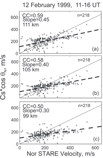
Figure 2 shows scatter plots of CS model predictions
ver-sus measured velocity for three heights. The format of the diagram is the same as in Fig. 1. The data show clear trends: with the height decrease, both the correlation coefficient and the slope of the best fit line deteriorate.
We should note that Uspensky et al. (2003) expected the scatter heights to be around 110 km for this event; at smaller heights the electron density was often too low to receive STARE echoes of significant power. One can conclude that the selection of the height of temperature measurements at 111 km in the CSmodel is the best choice for this event. This
selection might not be the correct one for all other events, though we believe that for the evening sector observations, which are considered in this paper, it is a reasonable one.
3 Analysis of the entire data set
To make a more reliable assessment of the CS model, we
identified a number of joint STARE/EISCAT events for which good quality data were obtained by both systems. Ta-ble 1 gives a summary of the events selected. Both EISCAT and STARE data sampling and averaging were the same as for the 12 February 1999 event.
3.1 Typical observational conditions
For all the above events, only measurements in the eastward electrojet were considered with positive (negative) Norway (Finland) velocities. The data statistics are smaller for the Finland radar as it detected very few echoes in the three events. In this section we consider MP data for both radars since we believe that they reflect the velocity of the electrojet irregularities better (Uspensky et al., 2005).
Figure 3 is a histogram presentation for the E×B velocity magnitude, ion-acoustic speed and flow angle, according to the EISCAT measurements for all events that were selected for a comparison with STARE velocity data, separately for
Fig. 2. A comparison of the predicted and measured velocity for
the Norway radar according to the model of Bahcivan et al. (2005). Three possible heights of backscatter are considered: (a) 111 km,
(b) 105 km and (c) 99 km.
the Norway and Finland radars. A total of 2085 (1379) joint points is available for the Norway (Finland) radar. The com-bined data statistics for both radars is almost 3 times larger than the one by Nielsen et al. (2002) and it is much more sig-nificant for the specific flow angles of 50◦–70◦. Bahcivan et al. (2005) had just several tens of points.
Figure 3 shows that the typical electron E×B velocity was ∼800–1200 m/s and the flow angle was ∼50◦–65◦(at
the level of 0.7 from the occurrence maxima). Since plasma drifts were enhanced, the observed values of CSwere larger
than the nominal speed of 400 m/s, as expected (e.g. Nielsen and Schlegel, 1985). The histograms of Fig. 3 mean that the selected data set corresponds to the same conditions as the one of Bahcivan et al. (2005). Nielsen et al. (2002) had gen-erally smaller E×B velocity magnitudes.
Table 1. Joint STARE/EISCAT events selected for the comparison.
Date Start-End Time Radar
(UT) 12 Feb 1999 11:00–16:00 N, F 11 Feb 1999 13:00–18:00 N 16 Sep 1999 10:00–18:00 N, F 17 Sep 1999 13:00–16:00 N, F 12 Oct 1999 09:00–17:00 N, F 13 Oct 1999 11:00–16:00 N 14 Oct 1999 13:00–16:00 N 15 Oct 1999 00:00–16:00 N, F
Fig. 3. Histogram distributions (a) for the E×B velocity
magni-tude, (b) the ion-acoustic speed at 111 km and (c) the flow angles of observations for the Norway and Finland radars in all events se-lected for the analysis. The total number of points is 2085 for the Norway and 1379 for the Finland radars. Data for the Norway (Fin-land) radar are shown by blue (green) color.
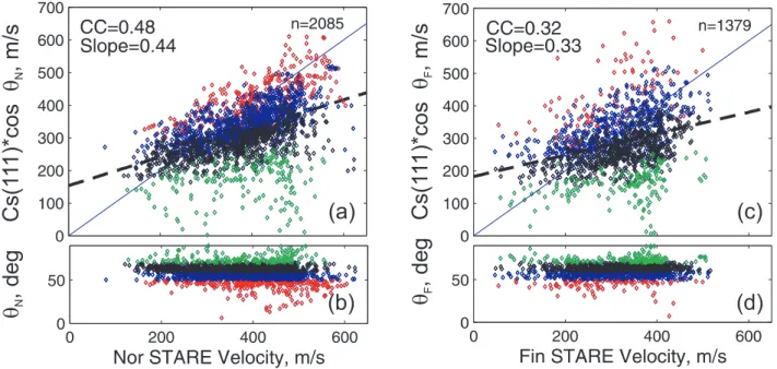
Fig. 4. The same as in Fig. 1 but for the entire data set of 8 (5) events for the Norway (Finland) radar. Coloring is made according to
10-degree bin of the flow angle of observations.
3.2 CSmodel expectations and measured velocities
Figure 4 presents CS-model predictions for both radars and
for all events considered. The format of the diagram is sim-ilar to the one of Fig. 1 , except here we coloured the points according to their flow angle: red, blue, black and green colours correspond to measurements in four different ranges of the flow angle, θ <50◦, 50◦<θ <60◦, 60◦<θ <70◦ and θ >70◦. Overall, the scatter plots are largely similar to the
ones presented in Fig. 1 just for one event. Comparing the Norway (left) column data and the Finland (right) column data, one notices that the point clustering and the correlation coefficients are somewhat better for the Norway radar but not significantly; the contrast is not as strong as the one for the 12 February 1999 event, implying that performance of the
CS model is very comparable for individual radars. Clearly,
for both radars, the predicted velocity is overestimated for low measured velocities (points are centered slightly above the bisector) and underestimated for large measured veloci-ties (points are below the bisector). Significant departures of the predictions and measurements occur for measured veloc-ities of >300 m/s, corresponding to ion-acoustic speeds of
>600 m/s. One can notice that the points corresponding to observations at 50◦<θ <60◦(blue colour) align better with
the line of ideal agreement. Most of the red points are lo-cated above the line of ideal agreement while most of the black and, especially the green points are located below this line.
4 Discussion
By considering joint STARE/EISCAT data we addressed the question of whether the ∼1-m irregularity phase velocity varies with the flow angle, as predicted by the CS model of
Bahcivan et al. (2005), Eq. (5). We involved a significant amount of measurements at flow angles of θ =50◦–70◦. The
correlation coefficient between the expected velocity and the measured one was found to be of the order of 0.4 and the slope of the best linear fit line to be of the order of 0.4. Both parameters are not very high and, technically, cannot be con-sidered as supporting the CS model. Perhaps, the exception
is for observations at flow angles of θ <60◦and measured ve-locities of 250–350 m/s (red and blue points in Fig. 4); these data can be rated as supporting the model. One should keep in mind, however, that the data are quite noisy and, in view of this, one cannot reject the CS model entirely, especially
because the other models do not perform overly strong. For both radars, the CSmodel underestimates (overestimates) the
measured l-o-s velocity for larger (smaller) velocities, as the points are located below (above) the line of ideal agreement. The trend at large measured velocities (large electron drifts) is especially obvious. The effect of the velocity underestima-tion at large flow angles would be even more pronounced if the height of scatter was in fact less than the assumed height of 111 km (the CS values drop down at these lower heights,
see data in Fig. 2 for 12 February 1999 event). If one assumes that the height of the scatter was above 111 km, the predic-tions can improve, but still the effect of underestimation is evident. For example, for the Norway radar, for the 12 Febru-ary 1999 event, if one suggests that the height of scatter was
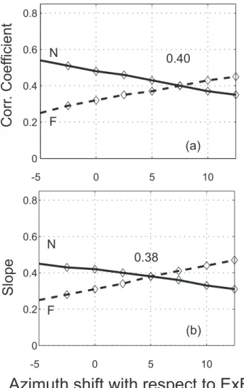
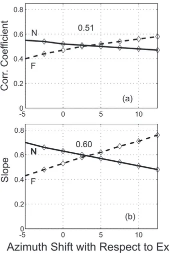
Fig. 5. The correlation coefficient and the slope of the best linear
fit line to observations for various shifts in the direction of the max-imum irregularity velocity. An irregularity velocity variation with the flow angle according to Bahcivan et al. (2005) was assumed. The positive shift corresponds to the CW direction from E×B.
114 km, the correlation coefficient and the slope of the best linear fit line are 0.55 and 0.39, respectively. These values are slightly worse as compared to the ones for the 111-km height of backscatter. For large flow angles (black and green points in Figs. 4a, d), the CS model clearly underestimates
the velocity almost in the entire range of observed velocities 200–500 m/s, even for the 111-km height of backscatter. The situation worsens if the scatter height is below 111 km.
The reason for some velocity underestimation within the
CS model, especially for larger flow angles, is not clear.
One might think that perhaps the maximum velocity CS is
achieved not at the E×B direction, as some theories ex-pect (e.g. Janhunen, 1994; St-Maurice and Hamza, 2001). To evaluate such a possibility, we computed the correla-tion coefficient and slope of the best fit line to the data by assuming shifts in the flow angle of the irregularity phase
Fig. 6. The same as in Fig. 4 but for predictions based on the
em-pirical equation of Nielsen et al. (2002).
velocity maximum and the E×B direction, θ0(positive an-gle θ0was assigned to the direction rotated clockwise (CW) from E×B). The results are presented in Fig. 5. One can see that the CS model predictions improve for the Finland
(Norway) radar with an increase (decrease) of θ0. A com-promise between the two radar sets seems to be achieved at
θ0∼5◦in the clockwise direction. This shift is in the opposite direction with respect to the predictions by Janhunen (1994). To conclude, one can say that the potential effect of the shift between E×B and the direction of maximum irregularity ve-locity does not improve the quality of the predictions with the
CSmodel.
In a just published theoretical paper, Bahcivan and Hy-sell (2006) considered a modified CSmodel. They suggested
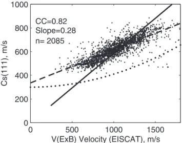
Fig. 7. A comparison of the measured ion-acoustic speed at 111 km
and the predicted one from the empirical equation by Nielsen and
Schlegel (1985). The dependence V =βVE (β=0.588) used in the
model by Uspensky et al. (2004) is shown by the solid line.
(whose velocity is Voi). This assumption implies that a term
of the order of ≈|Voi|cos φ should be added to Eqs. (5). We
performed estimates of the effect by considering the exact orientation of the ion velocity vector at 110 km with respect to the STARE radar beams. We found that for the Norway radar, the slope of the best linear fit decreases significantly to 0.16. For the Finland radar, the slope improves to 0.8, but the entire cloud of points shifts well above the expected bi-sector of perfect agreement between predictions and STARE observations. Our conclusion is that the modified model of Bahcivan and Hysell (2006) does not perform better than the simple CSmodel (5).
Another obvious concern is whether the irregularity phase velocity indeed changes with the flow angle according to the cosine function, Eq. (5). Nielsen et al. (2002) reported quite a different variation, Eq. (4). We performed velocity pre-dictions according to Eq. (4), Fig. 6. In Fig. 6a we present the variation of the coefficient proportionality in front of the cosine function in Eq. (4) versus flow angle, according to Nielsen et al. (2002). In Figs. 6b, c we compare predictions and measurements. The scatter plots in Figs. 6b, c have the same format as in Figs. 4a, c. In this case, overall, the ve-locity is slightly overestimated, as the majority of points are located well above the line of ideal agreement. The slope of the best fit line is better than in the case of the CSmodel. The
black points, corresponding to 60◦<θ <70◦, demonstrate the
best agreement.
Overall, one can say that the empirical Eq.(4) given by Nielsen et al. (2002) describes reasonably well the measured l-o-s velocity of ∼1-m irregularities at large flow angles, with about the same degree of success as the CSmodel of
Bahci-van et al. (2005). We should warn that Nielsen et al. (2002)
used DP velocities for both STARE radars (the pulse sep-aration was 300 µs). They merged them into one data set which might affect the conclusions in view that Uspensky et al. (2005) reported different ratios of the DP velocity to the MP velocity for the Finland and Norway radars, implying that the radars are not equivalent. Clearly, more deliberate investigation is required to decide whether the velocity de-pendence on θ is indeed a simple cosine function.
There are other areas of concern with the CS model.
Ac-cording to Chen et al. (1995) and Nielsen et al. (2002), the measured velocity of ∼1-m irregularities is above CS in a
broad range of flow angles, a fact that is completely ignored once Eq. (5) is adopted. In this respect, though, it is not clear what determines the flow angles for which type 1 irregulari-ties are excited within the scenario of Bahcivan et al. (2005). Also, the CS model predictions are only applicable to
rela-tively fast flows; what the expectations are for the irregular-ity velocirregular-ity below that FB instabilirregular-ity threshold (∼ 400 m/s) is unclear. Finally, there is difficulty in explanation of the velocity over-speed effect (Uspensky et al., 2003).
We would like to discuss one issue that is important to other studies in which the CS model is used. For the correct
model application it is essential that the ion-acoustic speed is estimated properly. Despite the fact that several papers have been devoted to the statistical study of the electron tempera-tures in the E-region (e.g. Jones et al., 1991), none of them presents a simple recipe as to how to estimate CS at
vari-ous heights for given electron velocity magnitude. Nielsen and Schlegel (1985) derived an empirical quadratic equation relating the STARE radar velocity at θ <θ∗ and the electron flow velocity magnitude
Vr =300 + 0.00011 · VE×B2 . (6)
They implied that Eq. (6) also gives an estimate of CS. One
has to always remember, however, that this formula is de-rived for the height of temperature observations of 105 km. It should also be modified if one uses it for morning sector measurements (Nielsen and Schlegel, 1985).
To assess how accurately Eq. (6) describes our observa-tions, we plotted in Fig. 7 the experimental points (EISCAT) and overlaid the dependence CS(VE×B)given by Eq. (6), as
heavy dots. One can recognize in a cloud of points a clear increase in CS with VE×B, as expected from pervious
stud-ies, e.g. Jones et al. (1991). The empirical Eq. (6), the dotted line in Fig. 7, also shows this trend, but it gives consistently smaller CS for all electron drift magnitudes. A similar
com-parison is somewhat better for experimental points at 105 km and even better for points at 99 km.
We would like to point out that according to Fig. 7, one would not expect STARE radar velocities to be larger than 800 m/s, the maximum observed CS values. We note that
the CS value of 600 m/s, the critical value starting from
which the CS model predictions start to significantly
of 1000 m/s. Schlegel and Thomas (1988) reported ∼1-m ir-regularity phase velocities larger than 1000 m/s which is in-consistent with the CSmodel unless the nonisothermality of
electron and ion motions in FB waves is considered (Farley and Providakes, 1989). Even larger velocities of ∼3-m irreg-ularities, as large as ∼2000 m/s, were reported by Unwin and Cummack (1980) in their 14 months of observations in the Southern Hemisphere over Campbell Island, geomagnetic latitudes of 59◦–63◦. They observed high-velocity “spikes” in a band of echoes extending 1◦–1.5◦in magnetic latitude, at the equatorward edge of low density E-layer structures (∼1010m−3), primarily in the pre-midnight sector. A quick scan through the accessible STARE DP data bank also re-vealed that the Norway and Finland l-o-s velocities can be as large as ∼1400 m/s and ∼1000 m/s, respectively, for exam-ple, on 18 April 2001 at 04:01–04:03 UT (morning sector).
Since the data presented do not support the CS model
un-doubtedly, we decided to look at other possibilities discussed in the Introduction. One of the widely circulated opinions is that the ∼1-m irregularity phase velocity is simply the cosine component of the E×B electron flow at θ >θ∗ (e.g. Nielsen et al., 2002). We consider predictions based on this assumption in Figs. 8a, b (Norway and Finland radars, re-spectively) which are scatter plots similar to Fig. 4. In this case, the correlation coefficients and the slopes of the best fit line are better as compared to the CS model ones, but the
clouds of points are sitting well above the bisectors, indicat-ing that Eq. (1) severely overestimates the measured veloc-ity of irregularities. This result means that the irregularveloc-ity phase velocity is smaller than the radar l-o-s component of the E×B velocity, which is in line with earlier findings (e.g. Koustov et al., 2002; Uspensky et al., 2004).
Another possibility in explaining the data is to use the full expression for the irregularity phase velocity at a cer-tain height, with the ion motion term and the aspect angle effect taken into account according to Eq. (3) (e.g. Kohl et al., 1992). Results of predictions based on this assumption and the scatter height of 110 km are presented in Figs. 8c, d. One can see that the agreement between predictions and observations is now much better, especially for the Finland radar. The predicted velocity for the Norway radar is strongly underestimated in this case contrary to the velocity overesti-mation for the Finland radar.
Finally, to explain the relationship between the STARE velocity and electric field at large flow angles, Uspensky et al. (2003, 2004) assumed that the irregularity phase veloc-ity follows the full linear dispersion equation for the unsta-ble FB waves (Eq. 3) and the irregularity layer is relatively thick, so that the resultant auroral echo is a combination of scatter from various heights. In a first approximation, such a model, termed the off-orthogonal fluid approach (OOFA) model by Uspensky et al. (2003), assumes Eq. (2) with val-ues of β of the order of 0.55 (Uspensky et al., 2004). We ap-plied the OOFA model to the data set available in this study, Figs. 8e, f. We used here Eq. (2) with β=0.588. This choice
of β is slightly different from the earlier recommendation by Uspensky et al. (2004) of β=0.55. The reason for our se-lection is that we used MP data for the Norway radar. The DP Norway velocities, used by Uspensky et al. (2004), are
∼1.1 times smaller than the MP velocities as was shown re-cently by Uspensky et al. (2005). Figures 8e, f show that the OOFA predictions (based solely on EISCAT data) agree rea-sonably well with the STARE velocity measurements. Ob-servations at θ < 60◦ (red and blue points) exhibit better agreement. Comparing the OOFA predictions (Eqs. 2, 3), Figs. 8e, f, with the simple E×B component assumption (Eq. 1), Figs. 8a, b, one can see that the cloud of points is rea-sonably well positioned with respect to the bisector, so that there is no systematic velocity overestimation effect. Com-paring the correlation coefficients and slopes in Figs. 8e, f with the ones given in Figs. 4a, c for the CS model, one can
notice an overall better performance of OOFA and especially for the Finland radar. This is evident in both parameters. The OOFA predictions look better than the ones based on the full linear theory applied to a specific scatter height of 110 km (Figs. 8c, d), in the sense that the predictions for both radars are reasonable. We can conclude that the OOFA model pre-dictions describe the experimental velocity data (considered in this study) better than the simple l-o-s component assump-tion and somewhat better than the other theories, namely the
CS model of Bahcivan et al. (2005), the model based on the
equation by Nielsen et al. (2002) and the model assuming a scatter from one single height of 110 km.
On the technical side, comparable performance of the CS
and OOFA models can be understood as follows. The dif-ference between these models – see Eqs. (2) and (5) – lies in the coefficients in front of the cosine function. Both co-efficients increase with the electron drift, and one generally would not expect any agreement between predictions be-cause the dependence CS(VE×B)is quadratic (Nielsen and
Schlegel, 1985, with a mean slope of ∼0.27, while the de-pendence β(VE×B)is linear with a slope of ∼0.6. To
illus-trate the differences between the models, we plot the function
V =βVE×B (β=0.588) in Fig. 7 by a solid line and also
indi-cate the best linear fit line to the CS measurements, a dashed
line. The dashed and solid lines in Fig. 7 do not coincide, but the significant differences between the two are evident only for the electron drifts of <600 m/s and >1200 m/s, cor-responding to a fraction of the all the data considered.
In passing, we can conclude from Fig. 7 that the OOFA model should predict larger velocities than the CS model at
strong electron drifts of >1300 m/s and smaller velocities for weak flows < 500 m/s. Examination of the Norway data in Fig. 4a supports this expectation. For the Finland data, the effect is less evident perhaps because of the generally smaller range of the measured velocities.
Better performance of the OOFA model does not mean that Eq. (2), or better yet Eq. (3), should be accepted as the one adequately describing the phase velocity of the ∼1-m electrojet irregularities at large flow angles, because both the
Fig. 8. The same as in Fig. 4 but for predictions based on the assumption that the irregularity phase velocity is the line-of-sight component
of the E×B electron drift, panels (a) and (b), on the assumption that the observed velocity is described by the linear fluid theory applied to the height of 110 km, panels (c) and (d), and on the assumption that the observed velocity is the l-o-s E×B component scaled down because of the aspect angle effect and echo reception from various heights (Uspensky et al., 2004), panels (e) and (f).
correlation coefficients and slopes are not close to 1. More-over, for large measured velocities of >500 m/s, the velocity predictions based on EISCAT data are above what is mea-sured, for both STARE radars. We think that perhaps the kinetic effects for the irregularity phase velocity need to be considered (Schlegel, 1983). If these effects are taken into account, the predicted irregularity phase velocity would be slightly smaller (than the velocity according to the fluid the-ory) and the match with STARE measurements would be
better at large measured velocities (electron drifts). Alter-natively, perhaps indeed at large drifts the velocity depen-dence on the drift magnitude is nonlinear, because the plasma turbulence becomes stronger and stronger. One effect that we have in mind is a change in the electron collision fre-quencies with an increase in the electron temperature (in-crease in the electric field magnitude). Our preliminary es-timates show that by allowing the coefficient β to vary with the electric field, agreement between the OOFA predictions
and observations can be improved significantly. In this case, simple OOFA estimates based on a fixed β are a useful ref-erence frame to reveal nonlinear dependence at fast electron flows. Careful investigation of the effect is the subject of a forthcoming paper.
In criticism of the OOFA model, one can point out that it consistently shows the slopes smaller than 1 at all flow an-gles, and this effect must be explained. In an attempt to un-derstand it, we investigated the potential role of the ion mo-tion contribumo-tion term in Eq. (3). This effect is expected to be important at large flow angles. First, we found that if points with very large flow angles of >70◦are removed from the statistics, the OOFA predictions improve, correlation coeffi-cient becomes CC=0.58 (0.56) and the slope becomes 0.64 (0.63) for the Norway (Finland) radar. As a second step, we investigated the possibility of a shift in the direction of the ir-regularity phase velocity maximum with respect to the E×B direction. We remind the reader that this is the major ex-pected effect of the ion motion (Uspensky et al., 2003). Fig-ures 9a, b shows the variation of the correlation coefficient and slope of the best linear fit line for OOFA predictions ver-sus the shift angle θ0. A positive angle θ0 corresponds to the CW rotation from the E×B direction. One can see that a compromise in predictions for both radars is achieved for a minor positive CW shift of ∼3◦. This result implies an in-significant role of ion motions for the flow angles of 50◦–70◦, so that other factors should be considered in explaining the OOFA velocity underestimation.
We think that an effect important for understanding the OOFA velocity underestimation has been considered by Us-pensky et al. (1989). These authors investigated the conse-quences of different STARE and EISCAT radar scattering volumes; a coherent radar averages over a significant volume while incoherent radar measures are a tiny area of the iono-sphere. If the electron density and electric field anticorrelate, which is reasonable to assume for the evening sector obser-vations, then according to Uspensky et al. (1989), the coher-ent radar would measure 10–20% smaller velocity, since, in the total received signal, the weight of the sub-areas with a smaller electric field would dominate.
We are not aware of theoretical work supporting the as-sumption that the ∼1-m irregularity phase velocity is close to the one predicted by the linear theory (with perhaps ion kinetic effects taken into account) at large flow angles. The theory of weak turbulence based on a three-wave interaction assumes this and can be used for justification of the OOFA assumption, though it is not clear to what extent one can use it for strongly driven electrojet conditions. Volosevich and Galperin (1997) proposed a new theory of soliton-like struc-ture formation. The velocity of such strucstruc-tures is propor-tional to the electron drift and the plasma turbulence level (or irregularity intensity). For large electron drifts/electric fields, the amplitude of electrojet irregularities is saturated (e.g. Nielsen et al., 1988), implying that the velocity should be proportional to the electron drift velocity. Thus this theory
Fig. 9. The same as in Fig. 5, except for the model based on the
assumption that the observed STARE velocity is the l-o-s compo-nent of the E×B drift scaled down due to the aspect angle effect and echo reception from various electrojet heights (Uspensky et al., 2004).
gives some support to the linear theory formula. Obviously, more theoretical work is needed.
Finally, we would like to mention that in order to decide more definitively whether the OOFA or the CS model better
describes the velocity of electrojet irregularities at large flow angles, further tests are needed. One should focus on mea-surements at very large electron drifts >1500 m/s for which the models’ predictions are quite different. It is also impor-tant to study more thoroughly observations at very large flow angles for which all considered models give an underestima-tion of the velocity (green points in Figs. 4, 6 and 8). Also, al-though EISCAT and STARE are very good instruments at the present time, we believe that future coherent radars with bet-ter spatial resolution and new phased-array incoherent scatbet-ter radars with multi-beam observations can provide data col-lected with comparable spatial resolution. This would, at least partly, decrease the data spread on diagrams similar to Figs. 4, 6 and 8.
5 Conclusions
We considered in this study STARE radar velocities and EIS-CAT data on the electron E×B velocity and ion-acoustic speed in the scattering volume of STARE observations. For a number of events in the afternoon and evening sectors (east-ward electrojet) with electron drifts of 400–1500 m/s and flow angles of 50◦–70◦we showed that:
1. The hypothesis of Bahcivan et al. (2005), that the elec-trojet irregularity phase velocity is the product of the ion-acoustic speed and the cosine of the flow angle of observations gives the correlation coefficient between measurements and predictions of ∼0.4, and the slope of the linear fit line of ∼0.4. The overall dominating tendency for the underestimation of the irregularity ve-locity is especially pronounced at large E×B drifts of
>1000 m/s.
2. The velocity estimates based on the Bahcivan et al. (2005) hypothesis are of better quality if the con-sidered flow angles are less than 60◦. The estimates de-teriorate if the actual height of the echoes is assumed to be less than 111 km.
3. The irregularity phase velocity estimates, based on the assumption that it is the line-of-sight component of the
E×B electron drift, disagree severely with the actual
STARE data.
4. For the empirical equation of Nielsen et al. (2002) de-scribing the irregularity velocity variation with the flow angle, agreement between the predictions based solely on EISCAT data and STARE measurements is compara-ble in quality with the predictions based on the hypoth-esis of Bahcivan et al. (2005).
5. The observed STARE velocity is best predicted by as-suming that the irregularity phase velocity is the line-of-sight component of the E×B electron drift scaled down, due to the off-orthogonality of irregularity prop-agation (nonzero effective aspect angle of observations) and echo collection from various heights, by a factor of
∼0.5–0.6, as suggested by Uspensky et al. (2004). 6. Further experimental tests of theoretical predictions
with respect to the electrojet irregularity velocity vari-ation with the flow angle have to concentrate on obser-vations at E×B drifts of >1000 m/s and flow angles of more that 60◦. For these conditions, predictions of var-ious theories divert the most.
Acknowledgements. The STARE system was operated jointly by
the Max Plank Institute for Aeronomy, Germany, and the Finnish Meteorological Institute, Finland, in cooperation with SINTEF, University of Trondheim, Norway. EISCAT is an international facil-ity supported by Finland, France, Germany, Japan, Norway, Sweden and the UK. We thank J.-P. St-Maurice conversations with whom
gave us an initial impetus for this study. We also thank A. Ko-zlovsky for his help in handling the EISCAT data. This work was supported by the NSERC (Canada) grant to AVK and FMI funding to MVU.
Topical Editor M. Pinnock thanks two referees for their help in evaluating this paper.
References
Bahcivan, H., Hysell, D. L., Larsen, M. F., and Pfaff, R. F.: The 30-MHz imaging radar observations of auroral irregularities during the JOULE campaign, J. Geophys. Res., 110, A05307, doi:10.1029/2004/JA010975, 2005.
Bahcivan, H. and Hysell, D. L.: A model of secondary Farley-Buneman waves in the auroral electrojet, J. Geophys. Res., A01304, doi:10.1029/2005JA011408, 2006.
Chen, P-R., Yi, L., and Nielsen, E.: Variations of the mean phase velocity of 1-m ionospheric plasma waves with the plasma elec-tron temperature, J. Geophys. Res., 100, 1647–1652, 1995. Farley, D. T. and Providakes, J.: The variation with Te and Ti of the
velocity of unstable ionospheric two-stream waves, J. Geophys. Res., 94, 15 415–15 420, 1989.
Fejer, B. G. and Kelley, M. C.: Ionospheric irregularities, Rev. Geo-phys., 18, 401–454, 1980.
Foster, J. C. and Erickson, P. J.: Simultaneous observations of E-region coherent backscatter and electric field magnitude at F-region heights with the Millstone Hill UHF radar, Geophys. Res. Lett., 27, 3177–3180, 2000.
Haldoupis, C. and Schlegel, K.: Direct comparison of 1-m irregular-ity phase velocirregular-ity and ion-acoustic speeds in the auroral E-region ionosphere, J. Geophys. Res., 95, 18 989–19 000, 1990.
Janhunen, P.: Perpendicular particle simulation of the E
re-gion Farley-Buneman instability, J. Geophys. Res., 99, 11 461– 11 473, 1994.
Jones, B., Williams, P. J. S., Schlegel, K., Robinson, T., and Hag-gstrom, I.: Interpretation of enhanced electron temperatures mea-sured in the auroral E region during the ERRIS campaign, Ann. Geophys., 9, 55–59, 1991.
Kofman W. and Nielsen, E.: STARE and EISCAT measurements: Evidence for the limitation of STARE Doppler velocity observa-tions by the ion acoustic velocity, J. Geophys. Res., 95, 19 131– 19 136, 1990.
Kohl, H., Nielsen, E., Rinnert, K., and Schlegel, K.: EISCAT re-sults during the ROSE campaign and comparison with STARE measurements, J. Atmos. Terr. Phys., 54, 733–739, 1992. Kustov, A. V. and Haldoupis, C.: Irregularity drift velocity
esti-mates in radar auroral backscatter, J. Atmos. Terr. Phys., 54, 415– 423, 1992.
Koustov, A. V., Danskin, D. W., Uspensky, M. V., Ogawa, T., Jan-hunen, P., Nishitani, N., Nozawa, S., Lester, M., and Milan, S.: Velocities of auroral coherent echoes at 12 and 144 MHz, Ann. Geophys., 20, 1647–1661, 2002.
Makarevitch, R. A., Koustov, A. V., Sofko, G. J., Andre, D., and Ogawa, T.: Multifrequency measurements of HF Doppler velocity in the auroral E region, J. Geophys. Res., 107, doi:10.1029/2001JA000268, 2002.
Nielsen, E. and Schlegel, K.: Coherent radar Doppler measure-ments and their relationship to the ionospheric electron drift ve-locity, J. Geophys. Res, 90, 3498–3504, 1985.
Nielsen, E., Uspensky, M., Kustov, A., Huuskonen, A., and Kangas, J.: On the dependence of the Farley-Buneman turbulence level on ionospheric electric field, J. Atmos. Terr. Phys., 50, 601–605, 1988.
Nielsen, E., del Pozo, C. F., and Williams, P. J. S.: VHF coherent radar signals from the E region ionosphere and the relationship to electron drift velocity and ion-acoustic velocity, J. Geophys. Res., 107, doi:10.1029/2001JA900111, 2002.
Sahr, J. D. and Fejer, B. G.: Auroral electrojet plasma irregularity theory and experiment: A critical review of present understand-ing and future directions, J. Geohys. Res., 101, 26 893–26 909, 1996.
Schlegel, K.: Interpretation of auroral radar experiments using a kinetic theory of the two-stream instability, Radio Sci., 18, 108– 118, 1983.
Schlegel, K.: Coherent backscatter from ionospheric E-region plasma irregularities, J. Atmos. Terr. Phys., 58, 933–941, 1996. Schlegel K. and Thomas, E. C.: Reply, J. Geophys. Res., 93,
5987-5988, 1988.
St-Maurice, J.-P. and Hamza, A. M.: A new nonlinear approach to the theory of E-region irregularities, J. Geophys. Res., 106, 1751–1760, 2001.
Unwin, R. S. and Cummack, C. H.: Drift spikes: The ionospheric signature of large poleward directed electric fields at subauroral latitudes, IMS in Antarctica, Memoirs of National Institute of Polar Research, No.16, 72–83, 1980.
Uspensky, M. V.: On the altitudinal profile of auroral radar
backscatter, Radio Sci., 20, 735–739, 1985.
Uspensky, M. V., Koustov, A. V., Eglitis, P., Huuskonen, A., Milan, S. E., Pulkkinen, T., and Pirjola, R.: CUTLASS HF radar ob-servations of high-velocity E-region echoes, Ann. Geophys., 19, 411–424, 2001.
Uspensky, M., Koustov, A., Janhunen, P., Pellinen, R., Danskin, D., and Nozawa, S.: STARE velocities: Importance of off-orthogonality and ion motion, Ann. Geophys., 21, 729–743, 2003.
Uspensky, M., Koustov, A., Janhunen, P., Nielsen, E., Kauristie, K., Amm, O., Pellinen, R., Opgenoorth, H., and Pirjola, R.: STARE velocities: 2. Evening westward electron flow, Ann. Geophys., 22, 1077–1091, 2004.
Uspensky, M. V., Koustov, A., Sofieva, V., Amm, O., Kau-ristie, K., Schmidt, W., Nielsen, E., Pulkkinen, T., Pelli-nen, R., Milan, S., and Pirjola, R.: Multi-pulse and double-pulse velocities of STARE echoes, Radio Sci., 40, RS3008, doi:10.1029/2004RS003151, 2005.
Uspensky, M., Kustov, A., Williams, P. J. S., Huuskonen, A., and Kangas, J.: Effect of unresolved electrojet microstructure on measurements of irregularity drift velocity in auroral radar backscatter, Adv. Space Sci., 9, 119–122, 1989.
Volosevich, A. V. and Galperin, Y. I.: Nonlinear wave structures in collisionless plasma of auroral E region ionosphere, Ann. Geo-phys., 15, 890–989, 1997.