The Retrieval of Ice-Cloud Properties from Cloud Radar and Lidar Synergy

HAL Id: hal-00068951

https://hal.archives-ouvertes.fr/hal-00068951

Submitted on 12 Dec 2020

HAL is a multi-disciplinary open access

archive for the deposit and dissemination of

sci-entific research documents, whether they are

pub-lished or not. The documents may come from

teaching and research institutions in France or

abroad, or from public or private research centers.

L’archive ouverte pluridisciplinaire HAL, est

destinée au dépôt et à la diffusion de documents

scientifiques de niveau recherche, publiés ou non,

émanant des établissements d’enseignement et de

recherche français ou étrangers, des laboratoires

publics ou privés.

and Lidar Synergy

Claire Tinel, Jacques Testud, Jacques Pelon, Robin J. Hogan, Alain Protat,

Julien Delanoë, Dominique Bouniol

To cite this version:

Claire Tinel, Jacques Testud, Jacques Pelon, Robin J. Hogan, Alain Protat, et al.. The Retrieval of

Ice-Cloud Properties from Cloud Radar and Lidar Synergy. Journal of Applied Meteorology, American

Meteorological Society, 2005, 44, pp.860-875. �10.1175/JAM2229.1�. �hal-00068951�

The Retrieval of Ice-Cloud Properties from Cloud Radar and Lidar Synergy

CLAIRETINEL* ANDJACQUESTESTUD

Centre d’études Terrestre et Planétaires, Institut Pierre Simon Laplace, Paris, France

JACQUESPELON

Service d’Aéronomie, Institut Pierre Simon Laplace, Paris, France

ROBINJ. HOGAN

Department of Meteorology, University of Reading, Reading, United Kingdom

ALAINPROTAT, JULIENDELANOË,ANDDOMINIQUEBOUNIOL

Centre d’études Terrestre et Planétaires, Institut Pierre Simon Laplace, Paris, France

(Manuscript received 19 December 2003, in final form 20 October 2004) ABSTRACT

Clouds are an important component of the earth’s climate system. A better description of their micro-physical properties is needed to improve radiative transfer calculations. In the framework of the Earth, Clouds, Aerosols, and Radiation Explorer (EarthCARE) mission preparation, the radar–lidar (RALI) airborne system, developed at L’Institut Pierre Simon Laplace (France), can be used as an airborne dem-onstrator. This paper presents an original method that combines cloud radar (94–95 GHz) and lidar data to derive the radiative and microphysical properties of clouds. It combines the apparent backscatter reflectivity from the radar and the apparent backscatter coefficient from the lidar. The principle of this algorithm relies on the use of a relationship between the extinction coefficient and the radar specific attenuation, derived from airborne microphysical data and Mie scattering calculations. To solve radar and lidar equations in the cloud region where signals can be obtained from both instruments, the extinction coefficients at some reference range z0must be known. Because the algorithms are stable for inversion performed from range

z0toward the emitter, z0is chosen at the farther cloud boundary as observed by the lidar. Then, making an

assumption of a relationship between extinction coefficient and backscattering coefficient, the whole ex-tinction coefficient, the apparent reflectivity, cloud physical parameters, the effective radius, and ice water content profiles are derived. This algorithm is applied to a blind test for downward-looking instruments where the original profiles are derived from in situ measurements. It is also applied to real lidar and radar data, obtained during the 1998 Cloud Lidar and Radar Experiment (CLARE’98) field project when a prototype airborne RALI system was flown pointing at nadir. The results from the synergetic algorithm agree reasonably well with the in situ measurements.

1. Introduction

Covering permanently almost two-thirds of the earth (Paltridge 1974), clouds reflect solar radiation and

ab-sorb a significant part of the infrared radiation emitted by the earth. Thus they exert a large influence on our weather and climate. Ice clouds represent 30% of the global cloud distribution (Riedi et al. 2000), but they currently are not represented correctly in the numerical global and forecast models, mainly because of the in-complete knowledge about their dynamical and physi-cal properties (Cess et al. 1990, 1996). For these reasons one of the goals of the international scientific commu-nity is to achieve better information on the microphysi-cal, dynamimicrophysi-cal, and radiative properties of clouds.

A way to obtain this information is to use combined

* Current affiliation: Centre National d’études Spatiales, Tou-louse, France.

Corresponding author address: Claire Tinel, CNES, DCT/SI/

MO–BPI 811, 18 av. Edouard Belin, 31401 Toulouse Cedex 9, France.

E-mail: [email protected]

© 2005 American Meteorological Society

ground, space, or airborne remote sensing instruments. First, combinations of active and passive instruments have been deployed from the ground in the 1990s. Ma-trosov et al. (1992) used radar and infrared radiometer to retrieve ice-cloud particle sizes and water contents. Mace et al. (1998a) proposed a method combining a radar and an infrared interferometer; Kumagai et al. (2000) combined a cloud radar and a microwave radi-ometer.

Uttal et al. (1990) and Intrieri et al. (1990) have con-ducted preliminary comparisons of lidar and backscat-tering in cirrus clouds. Intrieri et al. (1993) have devel-oped one of the first studies combining radar and lidar backscatter to retrieve cloud properties. Their method employs the wavelength-dependent difference in back-scatter between a carbon dioxide lidar (10.6 ␮m), an X-band radar (3.2 cm), and a Ka-band radar (8.6 mm) (among others) to determine the effective radius of ice-crystal sizes. Thus they compare the theoretical and observed backscatter coefficients, but they assume that all cloud particles were solid ice spheres and limit the lidar retrievals to an optical depth of 1. Mace et al. (1998b) used radar and lidar data to describe the cloud structure. These methods use a gate-by-gate correction for the lidar backscatter that becomes unstable once the optical depth becomes larger than 0.2 or 0.3. Flamant et al. (2000) studied some cirrus cases using a similar method and concluded that the radar–lidar combina-tion had difficulty in retrieving small particles (with an effective radius of less than 20␮m) because of the lim-ited radar sensitivity. Wang and Sassen (2002) recently used a parameterization of ice water content and par-ticle size in a function of integrated instrumental pa-rameters. Other approaches that constrain lidar extinc-tion retrieval from radar informaextinc-tion (Donovan and van Lammeren 2001; Donovan et al. 2001; Okamoto et al. 2003), have been developed recently. Those meth-ods overcome the instability of a gate-by-gate correc-tion and use total lidar attenuacorrec-tion as well as the at-tenuation at each gate.

In this paper, we explore in detail the concept of an original retrieval algorithm combining lidar and radar data [improved from Tinel et al. (2000)] and use it on simulated data and on 1998 Cloud Lidar and Radar Experiment (CLARE’98) measurements. This algo-rithm is based on the use of a set of power laws, called an inverse model, between integrated microphysical and instrumental parameters. The method presented in this paper is similar to the one presented by Donovan et al. (2001) because they try to find the solution that minimizes variations in the ratio of some power of the radar reflectivity to some power of the lidar attenua-tion. The difference occurs in the choice of the least

fluctuation of one parameter—the retrieved particle size at the far end of the cloud for Donovan et al. (2001) and the particle number concentration for this new method. This method involves the N*0 parameter. For a

better understanding, a summary of the concept of the “normalized” distribution to describe particle spectra developed by Testud et al. (2001) is explained in section 2. In section 3 the method combining radar reflectivity and lidar backscattering coefficient to retrieve cloud microphysical parameters, such as liquid water and ice water contents, and radiative parameters, such as the effective radius, is described. In section 4 the accuracy of algorithm retrievals is tested in a “blind” test. In section 5 the algorithm is applied to CLARE’98 data, when the first prototype airborne radar–lidar system was flown, and results are discussed.

As shown by Donovan et al. (2001), cloud radar–lidar synergy cannot retrieve an effective radius lower than 10 ␮m. This algorithm can be applied to high clouds where the lidar signal is strong enough to penetrate deep into the clouds and midlevel clouds with optical depth smaller than 4.5 (Tinel 2002).

2. Inverse model for radar and lidar retrieval

This section describes the concept of “normalized” particle size distribution developed by Testud et al. (2001), which aims to describe as accurately as possible the mean particle spectra. Parameters defining the re-sponse of active remote sensing instruments are the radar reflectivity Ze, the radar specific attenuation K,

the lidar backscattering coefficient␤a, and the lidar

ex-tinction coefficient ␣. They are by definition propor-tional to the moments of particle size distribution (PSD). Relationships between those parameters and microphysical parameters relevant to the evaluation of the cloud radiative properties [ice water content (IWC) and effective radius reof particles] can thus be

estab-lished.

The physical characterization of an observed cloud PSD raises the following question: What are the best parameters to use to characterize the mean particle size and the shape of the PSD?

The ice water content can be related to the cloud particle size distribution N(D), where D is defined as the particle diameter. Its expression is complex because it depends on particle density and shape. We will use hereinafter the formulation of Francis et al. (1998), who calculate the IWC from the microphysical obser-vations as IWC⫽␲␳w 6

冕

₀ ⬁ N共Deq兲Deq 3 dDeq, 共1兲

where Deq is the “equivalent melted diameter” (the

diameter that the ice particle would have if it were completely spherical and with a constant mass density), ␳wis the density of water, and N(Deq)dDeqis the

num-ber concentration of particles with diameters between

Deqand Deq⫹ dDeq. The Deqis empirically related to

the cross-sectional area A of the ice particle observed by the 2D probe through (Francis et al. 1998)

Deq⫽ 1.097A 0.50

for Aⱕ 0.0052 mm2 and

Deq⫽ 0.615A

0.39 _{for A⬎ 0.0052 mm}2_{. 共2兲}

Those relations were obtained from the 1993 European Cloud Radiation Experiment (EUCREX’93) in situ data when midlatitude cirrus clouds were sampled by 2D probes.

The characterization of the mean particle size is more difficult. McFarquhar and Heymsfield (1998) reviewed the different expressions of effective radii of particles according to their shape and phase. In our paper, the general form defined by Francis et al. (1994) is used:

re⫽共3⫻ IWC兲Ⲑ共2␳i␣兲, 共3兲

where␣ is the optical extinction and ␳iis the density of

ice, equal to 0.917 g cm⫺3. In what follows, the mean particle size is characterized by the “mean volume-weighted diameter” (usually referred to as the “mean volume diameter” in the literature), defined as

Dm⫽ M4ⲐM3, 共4兲

where M4and M3denote the fourth and third moment

of the PSD in Deqfor ice particles. Using the previous

definitions, the general expression of the PSD (Testud et al. 2001) is defined as

N共Deq兲⫽ N*0F共DeqⲐDm兲, 共5兲

where N*0is the normalization parameter of the particle

concentration, Dm is the normalization parameter of

the particle diameter, and F(X ) is the “normalized PSD” describing the “intrinsic” shape of the PSD (not-ing X⫽ Deq/Dm). Here N*0 is calculated using IWC and

Dm, which are calculated from the moments of the

PSD: N*0⫽ 44 ␲␳w IWC Dm 4 共6兲

(see Testud et al. 2001), where␳wis water density (⫽10

6

g m⫺3). Here, N*0 is physically interpreted as being

equal to the value of the N0parameter from an

expo-nential distribution with the same IWC and Dm.

In situ data have been collected by aircraft during CLARE’98, which took place in England in the au-tumn of 1998 (Illingworth et al. 1999) and the 1999

Cloud Airborne Investigation by Radar and Lidar (CARL’99), which took place in France in the spring of 1999 (Pelon et al. 2001).

CLARE’98 was devoted to the characterization of the microphysical, radiative, and dynamic properties of nonprecipitating clouds. For this purpose a ground-based combination of cloud radar, lidar, and radiom-eters has been deployed, as well as airborne instrumen-tation, including in situ microphysics and active remote sensing sampling. The C130 aircraft from the Met Of-fice was equipped with forward-scattering spectrometer probes (FSSP) and 2D cloud (2D-C) and 2D precipita-tion (2D-P) probes. The aircraft was flying in liquid-, ice-, and mixed-phase clouds. In this dataset, nine legs over 3 days have been considered: eight flights on 14 and 20 October (mixed-phase clouds) and one leg (cir-rus clouds) on 21 October 1998. In situ measurements have been made at different temperatures (⫺7°, ⫺10°, ⫺14°, and ⫺31°C); approximately 84 min of ice-cloud data with an integration time of 5 s have been extracted for our analysis.

The CARL’99 campaign was devoted to the investi-gation of ice-cloud properties and involved ground-based lidar, radar, and radiometric measurements, as well as in situ measurements from airborne probes. The Merlin IV aircraft from Météo France was equipped with FSSP, 2D-C, and 2D-P probes from the GKSS (Institute for Atmospherics Physics, in Germany). On 29 April and 4 May 1999, the aircraft was flying in cirrus clouds with respective temperatures of ⫺36° and ⫺21°C. Sampled data were mainly constituted of small aggregates. This dataset corresponds to 130 min of data (integration time 10 s) in our analysis.

This study concerns midlatitude ice clouds. Studies using in situ microphysical data from other field cam-paigns (midlatitude and tropical experiments) are also being performed at the Centre d’études Terrestres et Planétaires (CETP) and involve a global dataset of more than 150 h.

If Miis defined as the ith moment of the PSD [Mi⫽

兰 N(Deq)D

i

eq dDeq] and ␰i as the ith moment of the

normalized distribution [␰i⫽ 兰 F(X)X i

dX ], Mican be

rewritten, using Eq. (5), as

Mi⫽

冕

N*0F共DeqⲐDm兲Deq

n

dDeq⫽ N*0Dm i⫹1_␰

i. 共7兲

Thus the various Mimoments can be related to each

other with relations that are independent from the PSD shape: Mi N*0 ⫽␰i␰j⫺共i⫹1Ⲑj⫹1兲 Mj 共i⫹1Ⲑj⫹1兲 N*0 . 共8兲

The data described above have been used to calcu-late the various PSD moments and thus microphysical parameters (IWC, Dm, N*0) and parameters related to

radar and lidar (equivalent reflectivity Ze, radar

attenu-ation K, and optical extinction␣). At 94 GHz the effect of Mie scattering is to reduce the reflectivity of the larger particles below that predicted by Rayleigh theory, with the result that the mode in the reflectivity-weighted size distribution typically lies between 0.4 and 2 mm in diameter. This ensures that statistical sampling issues are not a concern when calculating 94-GHz re-flectivity from aircraft size spectra. The 2D-P probe measures particles of diameter up to 6.4 mm, and, from the sample volumes given by Heymsfield and Parrish (1978), a volume of 0.65 m3_{would be sampled in the 5-s}

integration interval used in CLARE’98. On average, over 800 particles between 0.4 and 2 mm were sampled every 5 s, providing a more-than-adequate sample from which to calculate reflectivity. Both Zeand K are

cal-culated in the Mie scattering:

Ze⫽ ␭4 1018 ␲5_|K w| 2

冕

N共D兲␴r共␭, D兲dD, 共9兲 where|Kw|

2_{is the dielectric factor of water (⫽0.17 for}

ice; Lhermitte 1987), ␴r is the particle backscattering

cross section, and D is the particle diameter measured by the probes, and

K⫽ 10

4

ln10

冕

N共D兲␴a共␭, D兲dD, 共10兲

where␴ris the particle attenuation cross section.

Op-tical extinction is proportional to the second moment of the PSD:

␣ ⫽␲₂

冕

N共D兲D2dD, 共11兲

where it is assumed that the lidar wavelength is small in comparison with the particle size and the geometric optics approximation can be applied.

Figure 1a shows the equivalent reflectivity Ze

(calcu-lated for a 95-GHz radar) versus the IWC. If Ze and

IWC are normalized by N*0, a much more stable

rela-tionship that can be reasonably parameterized as in Eq. (8) is obtained (see Fig. 1b):

IWC⫽ p共N*0兲1⫺qZe q

. 共12兲

As can be seen in Fig. 1a, a curvature in the power-law graphic representation appears when (Z/N*0)⬎ 10

8_.

This increase in slope observed in this domain is due to Mie effects (Van de Hulst 1957) that appear when par-ticles size D increases, especially when D/␭ ⬎ 0.08 (Bat-tan 1973). This corresponds to D ⬎ 250␮m for a

95-GHz radar. This makes it necessary to make a segmen-tation depending on Dmvalues in the establishment of

the power-law relationships.

The determination of similar relationships between the other integrated and microphysical parameters has then been established from in situ microphysical pa-rameters that were recorded during CLARE’98 and CARL’99 (Tinel 2002). They can be expressed as

IWC⫽ c共N*0兲 1⫺d_Kd and 共13兲 IWC⫽ e共N*0兲 1⫺e_␣f , 共14兲

which allows one to derive relationships between the integrated parameter themselves as

K⫽ a共N*0兲1⫺bZe b_{, 共15兲} ␣ ⫽ m共N*0兲 1⫺n_Kn , and 共16兲 ␣ ⫽ s共N*0兲1⫺tZe t_{. 共17兲}

Table 1 represents the values obtained for the differ-ent relationships applied to three Dmdomains defined

to be in the Rayleigh scattering regime (Dmⱕ 175␮m)

and in the non-Rayleigh regime—values for Dm⬎ 175

␮m and corresponding to Dm⬎ 400␮m were

differen-tiated to separate the scattering regimes. The three do-mains are specified on Fig. 1b.

3. Description of the radar–lidar synergetic algorithm

In this section the mathematical formulation of a syn-ergetic algorithm for radar and lidar is developed. In a dataset, common areas, where measurements from both a radar and a lidar are available, have to be se-lected for the analysis. This method is applicable to ice clouds, because the inverse model described in the pre-vious section has been derived for ice clouds. However, this algorithm could, in principle, be used for other cloud types, provided that a specific inverse model is developed and introduced in the algorithm. In addition, this formulation is valid for ground-based, airborne, or spaceborne applications.

a. Radar measurements

The radar does not measure the true reflectivity Ze,

but an attenuated reflectivity Zasubject to the two-way

path attenuation because of the attenuation at 95 GHz. Reflectivities Zaand Zeare related through

Za⫽ Ze⫻ 10⫺0.2兰0

r

K共s兲 ds_{, 共18兲}

where K (dB km⫺1) is the specific attenuation and r is the distance from the radar to the measurement

alti-tude. Variables Z and K are usually related in the lit-erature through a power-law relationship:

K⫽ a⬘Zb⬘. 共19兲

This power law is valid along the path; it assumes that the radar beam goes all of the way through the same

type of particles. Under this assumption, Hitschfeld and Bordan (1954) were the first to derive the exact solu-tion of the inversion of the solusolu-tion, expressed as

Ze共r兲⫽

Za共r兲

关1⫺ a⬘I共0, r兲兴1Ⲑb⬘, 共20兲

TABLE1. Coefficients of the power-law relationships corresponding to the three Dm(␮m) domains derived from in situ microphysical measurements collected by aircraft during CLARE’98 and CARL’99.

Dm(␮m)

domain a b c d e f m n p q s t

Dm⬎ 400 2.620⫻ 10⫺3 1.028 0.029 0.742 0.351 1.104 0.102 0.671 3.598⫻ 10⫺4 0.764 1.980⫻ 10⫺3 0.690 175⬍ Dm⬍ 400 8.890 ⫻ 10⫺7 0.594 0.102 0.793 0.613 1.135 0.180 0.693 1.620⫻ 10⫺6 0.471 1.222⫻ 10⫺5 0.415

Dm⬍ 175 2.010⫻ 10⫺7 0.547 0.407 0.407 1.019 1.164 0.314 0.710 9.304⫻ 10⫺7 0.459 6.634⫻ 10⫺6 0.395 FIG. 1. Illustration of (a) IWC (g m⫺3) vs Ze(mm6m⫺3) and (b) IWC (g m⫺3)/N*0 (m⫺4) vs

Ze(mm6 m⫺3)/N*0 (m⫺4) (for a 95-GHz radar) in a logarithmic scale for the CLARE’98/

CARL’99 microphysical dataset for temperatures varying from ⫺36° to ⫺7°C. In (b), the three Dmdomains (defined in section 2) are specified as follows: the lowest panel is 175␮m ⬎ Dm, the middle panel is 175␮m⬍ Dm⬍ 400␮m, and the top panel is Dm⬎ 400␮m.

where I共0, r兲⫽ 0.46b⬘

冕

0 r Za b⬘_共s兲ds.

This solution is numerically unstable, as recognized by the authors themselves. It allows the correction from the attenuation as long as the value of the attenuation is weak. When this value increases, however, the algo-rithm tends to diverge as the value of the denominator tends to 0. The solution of the equation is also subject to the values of a⬘ and b⬘, which increases its instability. Equation (20) may be reformulated with respect to the attenuation in the following manner (Testud et al. 1996): K共r兲⫽ K共r0兲N*0共r兲 1⫺b_Z a b 共r兲 N*0共r0兲 1⫺b_Z a b_共 r0兲⫹ 0.46bK共r0兲

冕

r r0 N*0共s兲 1⫺b_Z a b_共 s兲ds , 共21兲 where r0 is the far-end reference bound (r ⬍ r0) and

rewriting Eq. (20) in this manner allows us to obtain a stable scheme. We will see later how this boundary is determined in the proposed algorithm. The interest of this formulation is that it provides an expression for a K profile not subject to the radar calibration.

b. Lidar measurements

In a similar way, the lidar does not measure the true backscattering coefficient, but an apparent backscatter-ing coefficient ␤athat is related to␤ethrough

␤a⫽␤eexp

冋

⫺2

冕

0

r

␣共s兲ds

册

共km⫺1sr⫺1兲, 共22兲 where ␣ (km⫺1) is the extinction coefficient. The as-sumption of a linear law between␣ and ␤eis generally

made:

␤e⫽ k␣. 共23兲

The problem posed by the inversion of Eq. (22) is the same as that posed by the inversion of Eq. (20). Klett (1981) gave the exact solution of this inversion:

␤e共r兲⫽ ␤a共r兲 1⫺ 2

冕

r r0 关␤a共s兲Ⲑk共s兲兴ds . 共24兲

As in Eq. (20), this expression of the true backscatter-ing coefficient is numerically unstable because of the divergence when the denominator tends to zero. This solution does not impose to meet the same type of

par-ticles along the lidar beam, and k can vary with dis-tance.

The Klett solution may be also reformulated as a stable expression in terms of the extinction coefficient at the far side of the cloud␣(r0):

␣共r兲⫽ ␣共r0兲␤a共r兲 ␤a共r0兲⫹ 2␣共r0兲

冕

r r0 ␤a共s兲ds , 共25兲

where r0is the far-end reference bound (r⬍ r0). As for

the radar, it does not depend on the instrument cali-bration. Following the Klett assumption, k is assumed to be constant along the lidar beam. Because k depends on particle size, shape, and orientation, we assume that we have the same type of particles along the beam. This assumption has no effect on the parameter retrieval, as will be shown in section 4b. Its drawback is that it is subject to the determination of ␣ at the reference boundary, which may not be accurately known. To overcome this problem, an iterative procedure is devel-oped to combine radar and lidar data to derive the reference extinction coefficient, which is described hereinafter.

c. Determination of boundary values

Although we have seen that both (radar and lidar) inversions need to be performed from the far end of the measurement area, it is possible to constrain radar and lidar measurements in relation to each other to derive the boundary values.

Equations (21) and (25) respectively depend on K(r0)

and␣(r0). The following integral constraint along the

path of both instrument beams is used to determine those two entities:

冕

r1 r0 ␣共s兲ds⫽ m

冕

r1 r0 N*0 共1⫺n兲_共s兲Kn 共s兲ds. 共26兲

This constraint expresses the consistency of K(r) and ␣(r) profiles with the power-law relationship obtained by the inverse model described in section 2. Here, r0

and r1are the extreme heights at which lidar and radar

signals are both available; r0 is the farthest

measure-ment point from the instrumeasure-ments, whereas r1is the

near-est one. A function is introduced to stabilize the itera-tive process of the algorithm that is defined with

f共r兲⫽N*0共r兲 N*0

, 共27兲

where N*0 is the mean N*0 along the profile.

Replacing K(r) from Eq. (21) and␣(r) from Eq. (25) and Eq. (16), an implicit equation in␣(r0) is obtained

␣共r0兲⫽ ␤a共r0兲 2

冕

r0 r1 ␤a共s兲ds

冤

exp

冢

2 ␣共r0兲 f共r0兲 1⫺n

冕

r0 r1 f共s兲1⫺n

冬

f共s兲1⫺bZa b 共s兲 f共s兲1⫺bZa b_共r 0兲⫹

再

␣共r0兲 m关f共r0兲N*0兴1⫺n

冎

1Ⲑn I共s, r0兲

冭

n ds

冣

⫺ 1

冥

, 共28兲 where I共s, r0兲⫽ 0.46b

冕

s r0 f共r兲1⫺bZa b_共r兲dr.

The algorithm is initialized with a constant value of

N*0 (⫽10

10_{) and f(r)⫽ 1 that allows a computation of}

the first value of␣(r0). Then, a new one is determined

by solving Eq. (28) that allows the retrieval of a new extinction profile. Because this algorithm is suitable for ice clouds and because the radar attenuation is negli-gible in ice (mean value of 10⫺2dB km⫺1), the retrieval of the K(r) profile may be unstable because of the low values of the radar attenuation. Thus, a new N*0(r)

pro-file is calculated from optical extinction and Za(r)

[in-stead of Ze(r) because we assume that Za(r)⬇ Ze(r)],

and then a new profile of f(r). The process is finally iterated until the following convergence criterion based on the␣(r0) value is satisfied:|␣i⫹1(r0)⫺␣i(r0)| ⱕ 10⫺3

km⫺1. The algorithm usually converges in less than 10 iterations.

Once the final N*0 vertical profile is obtained, it is

possible to retrieve the ice water content profile using Eq. (12). Then, Eq. (3) is used to retrieve the particle effective radius by combining IWC and␣. The coeffi-cients of the power-law relationships used in the first step of the retrieval process are those corresponding to middle-sized particles (175␮m ⬍ Dm⬍ 400␮m). The

retrieval of IWC and N*0 in the convergence process

allows us to calculate a new mean Dmalong the profile,

and the coefficients corresponding to this mean value (from Table 1) are used in the next step. The criteria convergence used for the retrieval of␣ implies a rela-tive error in the retrieval of IWC that is lower than 12% for␣ ⱖ 0.01 km⫺1.

This retrieval algorithm aims to find the␣(r0) value

(or, equivalent, the optical depth or the K profile) that, when radar and lidar are combined, produces the N*0

profile that changes least with height. Because it is physically reasonable to assume that the concentration is fairly consistent as particles fall, the linking constraint between extinction profile and attenuation profile is a powerful constraint.

4. Application of the algorithm to a blind test

As mentioned in the introduction, one of the major unknowns in forecasting climate change concerns the

radiative impact of clouds. To reduce this uncertainty, the international scientific community is presently de-signing two space missions: Earth, Clouds, Aerosols, and Radiation Explorer [EarthCARE; the European Space Agency (ESA)–National Space Development Agency (under consideration)] and “CloudSat” [the National Aeronautics and Space Agency (NASA)– Canadian Space Agency]–Cloud-Aerosol Lidar and In-frared Pathfinder Satellite Observations [(CALIPSO); NASA–Centre National d’études Spatiales (CNES)]; CloudSat–CALIPSO is slated to be launched in the spring of 2005. The development and validation of the radar–lidar algorithm is naturally done in the frame-work of the preparation for these two missions. The validation of the algorithm has been conducted with a “blind test” exercise funded by ESA within the frame-work of EarthCARE mission performance studies. The goal of this test was to apply the synergetic algorithm on a set of data processed by satellite instruments. Sev-eral algorithms were involved in this test for intercom-parison purposes.

a. Blind-test scenario

A complete description of the blind-test conditions, results, and comparisons is given in Hogan et al. (2004, manuscript submitted to J. Atmos. Oceanic Technol.). We will concentrate here on the results obtained with our algorithm. A short presentation on the blind-test conditions is provided. The dataset (including five ver-tical profiles of various parameters of interested as de-scribed below) was initially built by R. J. Hogan of the University of Reading from in situ data collected by the Met Office C-130 aircraft during five Lagrangian de-scents in frontal clouds around the British Isles. The aircraft was equipped with Particle Measuring Systems, Inc., (PMS) 2D cloud and precipitation probes (diam-eter range 25–6400␮m), and the ice particle size distri-butions binned by cross-sectional area were used to cal-culate the five vertical profiles (for five Lagrangian de-scents; thus, 25 profiles in total): visible extinction coefficient␣, IWC, effective radius re, radar reflectivity

factor at 94 GHz (as seen from space), and lidar-attenuated backscatter (as seen from space). For each of the lidar-attenuated backscatter profiles, two profiles of extinction-to-backscatter ratio k were used (using hypothetic but consistent values)—one constant with

height and the other varying with height over approxi-mately a factor of 2, similar to the range found by Ans-mann et al. (1992). Multiple scattering has not been taken into account in this simulation.

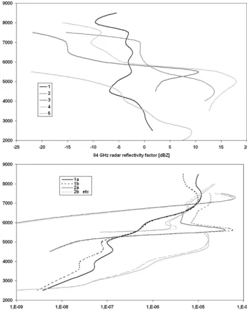
Figure 2 shows the 5 synthetic reflectivity (top panel) and 10 synthetic backscatter profiles (bottom panel; profiles labeled “a” have constant k, and profiles la-beled “b” have varying k with height), respectively, that were applied in the retrieval algorithm. No information on the k values had been provided before applying the synergetic algorithm to the synthetic profiles.

b. Results

Without having any information on the microphysi-cal profiles built from in situ microphysimicrophysi-cal data, the

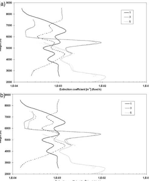
synergetic algorithm has been applied to the simulated apparent reflectivity and lidar backscatter profiles to retrieve IWC and reprofiles. Figures 3–5 show the

vis-ible extinction coefficient, ice water content, and effec-tive radius profiles (only for three of the five profiles to provide easier viewing; retrieval accuracies for profiles 2 and 4 are similar to the accuracies for profiles 3 and 5) initially built from the direct profile simulation and the corresponding values blindly retrieved by the algo-rithm. For each profile, there are two retrievals corre-sponding to the different k profiles used in the direct profile simulation (constant or varying with height). It is interesting to see that the retrievals in the case of k constant with height (Figs. 3a, 4a, and 5a) are fairly close to the true profiles in most cases, when the

re-FIG. 2. (top) Apparent cloud radar reflectivity and (bottom) backscattering lidar coefficient profiles as seen from space and derived from in situ measurements; “a” profiles have fixed k, and “b” profiles have variable k. In the bottom panel, 1,E⫺09 translates to 1.0 ⫻ 10⫺9, etc.

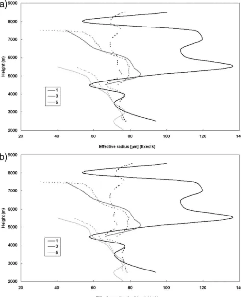
trieved profiles in the case of k varying with height are slightly different from the true profiles (Figs. 3b, 4b, and 5b). Mean biases are less than 10% in most of the cases, which reflects the independence of the algorithm from the value of the mean k profile and its small sen-sitivity to a variation in k. IWC and reare retrieved well

in all cases except for profile 1, for which retrieved parameters are clearly underestimated. This underesti-mation is due to the Mie effects that occur at 94 GHz (Van de Hulst 1957). Better accounting for these effects in the inverse model will reduce their impact even if presence of bias is unavoidable: Mie effects mean that reflectivity becomes a similar moment of the size dis-tribution as extinction and so ability to retrieve particle size is lost. Also, there is density dependence at Mie scatter. Because of the power-law relationships, a bias in the retrieved extinction parameter unavoidably

brings corresponding bias in the retrieved ice water content. This bias is compensated in the retrieved ef-fective radius due to Eq. (3), as shown in Fig. 4.

Figures 3–5 show that the retrieved reference values at the bottom of each profile (in the lowest few hundred meters) are different from the true values. This differ-ence is due to the hypotheses made in the use of the mathematical integral formulation [Eq. (26)]. Even if there is some uncertainty in the retrieval of␣(r0)

(im-plying disagreement of the retrieved profiles at the low-est boundary for an airborne or spaceborne platform as seen on Fig. 4), the integral formulation allows us to retrieve profiles that are reasonably close to the true ones above it. This situation is due to the increasing contribution of the optical depth, which reduces the error due to the reference.

Figure 6 shows the N*0 profiles retrieved by the

algo-FIG. 3. Realistic (solid lines) and retrieved (dotted lines) visible extinction coefficient derived from the blind test, with (a) fixed k and (b) variable k.

rithm from the simulated radar and lidar measurements (dotted lines) for k constant together with the “realis-tic” N*0 profiles calculated directly from the aircraft size

distributions (solid lines). The implication is that this representation mainly depends on coefficients used in the power-law relationships. It appears that N*0 may

vary by two orders of magnitude, which is equivalent to the recent results from in situ measurements reported by Heymsfield et al. (2002).

5. Application of the synergetic algorithm to CLARE’98 data

During CLARE’98 various observing systems were deployed for clouds and radiation at Chilbolton (En-gland) in the autumn of 1998. This ground-based

ex-periment (including various meteorological radars and passive microwave observations) was coordinated with flights of three aircraft: the C130 of the Met Office, the Deutschen Zentrum für Luft- und Raumfahrt Falcon, and the Fokker 27 Avion de Recherches Atmo-sphériques et de Télédétection (ARAT) of the French Institut National des Sciences de l’Univers (INSU). For the purpose of this paper, the joint C130 and ARAT flights are particularly interesting. The instruments used to obtain microphysical data in ice clouds were the PMS 2D-C and 2D-P probes (Francis 1999) mounted aboard the C130, and the ARAT was equipped with the 95-GHz Microwave Radar for Cloud Layer Explora-tion (MIRACLE) of the University of Wyoming (Pazmany et al. 1994), connected to the dual-beam an-tenna of CETP (looking alternately at nadir and at

FIG. 4. Realistic (solid lines) and retrieved (dotted lines) ice water content derived from the blind test, with (a) fixed k and (b) variable k.

about 45° forward), and with the nadir-looking Lidar Embarqué pour l’étude de l’Atmosphère: Nuages, Dy-namique, Rayonnement et cycle de l’Eau (LEANDRE) lidar operating at 0.5␮m (Sauvage et al. 1999).

The synergy between radar and lidar is particularly efficient when probing an ice cloud because the pen-etrations of the radar and the lidar in this type of cloud are generally comparable. The subsequent data analysis is focused on a particular leg (1441–1448 UTC 20 Oc-tober 1998) for which the ARAT was flying at 4.8-km altitude and the C130 was flying in cloud at 4.6-km altitude along the same leg.

Figure 7 shows measurements provided both by the radar (top panel) and the lidar (bottom panel). An iced cloud is observed between longitudes 1.95° and 1.65°W above approximately 3.2 km. Because of good

coordi-nation between the two aircraft, a very satisfactory co-incidence in space and time of the ground tracks of the two aircrafts was achieved on this leg. Between longi-tudes 2° and 1.7°W and above 3-km altitude, both in-struments (nadir looking) see the same cloud bound-aries, and the synergetic algorithm can be efficiently applied. To ensure that the lidar signal is not too noisy, the algorithm is applied by taking into account a mini-mal value of ␤a (equal to 2 ⫻ 10⫺3 km⫺1 sr⫺1) for

determining r0. Parameter r0is represented with a white

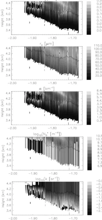
full line on Fig. 7 and with black full lines on Fig. 8. Figure 8 shows the parameters retrieved by the syn-ergetic algorithm. Values of IWC and re parameters

respectively range from 0.01 to 0.28 g m⫺3and from 30 to 110␮m. It appears that the algorithm diverges on the left part of the cloud (between 1.93° and 1.83°W

longi-FIG. 5. Realistic (solid lines) and retrieved (dotted lines) visible effective radius derived from the blind test, with (a) fixed k and (b) variable k.

tude), where the cloud thickness is less than 300 m [which is in agreement with the simulation results (Ti-nel 2002)]. Values obtained in the other part of the cloud are consistent with what is usually observed in ice cloud. Values of N*0 (m⫺4) and k (sr⫺1) range from 10

8

to 1010 and from 10⫺3 to 10⫺1, respectively. Even if there are some errors in the radar measurements, re-trieved parameter values are continuous in the part of the cloud where the algorithm converges. A constant value of N*0 is assumed below the black line [equal to

N*0(r0)], which allows retrieval of the other parameters

by using the inverse model. This assumption is realistic because of the small thickness of the cloud layer.

Figure 9 shows time series of the parameters re-trieved by the synergetic algorithm (Z, IWC, re,␣, and

N*0) along the ARAT track at the height of 4.48 km. As

in Fig. 7, values of IWC and reare consistent with what

is usually observed in ice clouds (mean value of 0.2 g m⫺3for IWC, and values ranging from 65 to 100␮m for re). Parameters are compared with in situ

micro-physical parameters calculated by P. Francis (1999, personal communication; represented by dotted lines). The agreement between radar/lidar retrievals and in

FIG. 6. Realistic (solid lines) and retrieved (dotted lines) N*0

derived from the blind test (k is constant).

FIG. 7. (top) MIRACLE radar apparent reflectivity and (bot-tom) LEANDRE lidar apparent backscattering coefficient during CLARE’98 for 1441–1448 UTC 20 Oct 1998.

FIG. 8. Vertical cross section of various parameters retrieved with the synergetic algorithm (CLARE’98, at 1441–1448 UTC 20 Oct 1998). From top to bottom: IWC, effective radius re, lidar extinction␣, normalization parameter N*0, and lidar ratio k.

situ measurements is good between 1.84° and 1.65°W. Beyond 1.84°W, the divergence of the algorithm, as mentioned before, is observed because of the strong lidar attenuation into the dense cloud part. To get rid of this divergence, another version of the algorithm that assumes a constant N*0 value within the cloud, which

substantially simplifies Eq. (19), has been applied. This assumption is realistic in this case because the cloud layer thickness is small, but it could not generally be used with a deeper cloud layer. Figure 10 represents the parameters obtained using this assumption. Retrieved values are similar to those retrieved by the profiling algorithm when it does not diverge and are close to the in situ measurements between 1.93° and 1.83°W longi-tude. This result validates, in particular, the assumption of a constant N*0 profile for small cloud-layer thickness

(less than 500 m; Tinel 2002).

6. Conclusions

The potential of cloud radar and lidar combination on the same platform is very promising. We have pre-sented in this paper a new synergetic algorithm, the formulation of which relies on a normalization

param-FIG. 9. Along-track evolution at 4.48 km during CLARE’98 experiment (1441–1448 UTC 20 Oct 1998). From top to bottom: radar reflectivity Ze, IWC, re, extinction coefficient␣, and PSD parameter N*0. Solid lines: synergetic algorithm; dotted lines: in

situ measurements.

FIG. 10. Vertical cross section of various parameters retrieved

with the synergetic algorithm for N*0 constant (CLARE’98, at

1441–1448 UTC 20 Oct 1998). From top to bottom: IWC, re, lidar extinction␣, normalization parameter N*0, and lidar ratio k.

eter N*0. The use of this parameter allows us to take into

account the natural variability of particle concentration in clouds. Simulation tests (Tinel 2002) and blind tests have shown the capacity of the algorithm to retrieve cloud parameters (with relative errors of less than 10% for optical extinction and ice water content). This algo-rithm has then been applied to real data from CLARE’98, and good agreement between the retrieved and in situ parameters has been obtained.

The aim of this paper was to describe a first version of a new and original radar–lidar algorithm. Because we assume that concentrations in large and small crys-tals are related, the application of the algorithm is lim-ited to the retrieval of effective radius larger than 20 ␮m and smaller than 200 ␮m. Because this algorithm requires a substantial lidar return, this technique is ap-plied to high clouds where the lidar signal is strong enough to penetrate deep into the clouds. This condi-tion means that radar reflectivities should not excess 20 dBZ (for a W-band radar). Effects of precipitation would not affect the radar signal too much but would often totally extinguish lidar signal, which is why this algorithm applies to nonprecipitating clouds. Equiva-lent radar/lidar methods exist for drizzle and liquid clouds (Baedi et al. 2000; O’Connor et al. 2004), and a companion version of this algorithm can be imagined for lightly precipitating clouds (such as the drizzling part of stratocumulus), where a lidar return is available. However, such an algorithm requires a specific inverse model. At this point, further developments of this al-gorithm should be directed toward the following:

• The segmentation of the analysis in the conditions in which different types of cloud are met along the beam should be investigated. For example, the leg just before the studied case in this paper was in a cloud with a thin supercooled layer embedded within the deeper ice stratus, and preliminary work has al-ready been done by Tinel (2002). We also often meet cases with multilayered clouds that have to be pro-cessed separately. Both configurations could be ac-counted for in the algorithm. For mixed-phase clouds, the radar will be essentially sensitive to the ice while the lidar will be essentially sensitive to the liq-uid water. This phenomenon is another complemen-tary aspect of the radar–lidar combination that needs to be explored (Hogan et al. 2003).

• The analysis should be extended to other microphysi-cal datasets to evaluate our inverse model and to document possible systematic variations of the N*0

parameter with altitude or normalized cloud height.

• The interest of using the terminal fall velocities re-trieved from the radar Doppler measurements (e.g.,

Protat et al. 2002) as an additional constraint to the algorithm should be investigated.

• The lidar measurements should be corrected for mul-tiple scattering, which is likely to contribute in a sig-nificant manner in some ice clouds. An analytical procedure proposed by Eloranta (1998) is now being tested in the algorithm.

• The Mie effects in the inverse model should be ac-counted for more precisely. Such an accounting may be done with a parameterization by Dmof the

coef-ficients of the power-law relationships.

• The information from microphysical probes on diam-eter and area, and not only on area, should be taken into account. The use of various density laws for the establishment of the inverse model may affect the IWC retrievals by a factor of almost 2. This effect is being taken into account through an extensive analy-sis of microphysical in situ measurements in both tropical and midlatitude regions (Delanoë et al. 2005).

The ground-based version of this algorithm has al-ready been implemented. It is being systematically ap-plied to the large ground-based database collected from three European cloud remote sensing stations [Cabauw, Netherlands, Site Instrumental de Recherche par Télédétection (SIRTA) in Palaiseau, France, and Chilbolton] that are equipped with cloud radar and li-dar in the framework of the European “CloudNET” project.

The spaceborne application of this algorithm obvi-ously needs to be explored soon. The adaptation of this version of the algorithm would require that simulations of the radar and lidar measurements from space be performed, with evaluation of the skills of the algo-rithms in this spaceborne configuration.

Acknowledgments. The authors are grateful to Peter

Francis at the Met Office and Dagmar Nagel at GKSS for providing in situ microphysical data. This research was funded by CloudNET project (EVK2-CT2000-00065) and ESA (15741/01/NL/SF). ESA, INSU, and CNES are acknowledged for their financial support of our participation in the CLARE’98 and CARL’99 field experiments.

REFERENCES

Ansmann, A., U. Wandinger, M. Riebesell, C. Weitkamp, and W. Michaelis, 1992: Independent measurements of extinction and backscatter profiles in cirrus clouds by using a combined Raman elastic-backscatter lidar. Appl. Opt., 3, 7113–7131. Baedi, R. J. P., J. J. M. de Wit, H. W. J. Russchenberg, J. S.

Erkelens, and J. P. V. Poiares Baptista, 2000: Estimating ef-fective radius and liquid water content from radar and lidar

based on the CLARE’98 data-set. Phys. Chem. Earth, 25, 1057–1062.

Battan, L. J., 1973: Radar Observations of the Atmosphere. Uni-versity of Chicago Press, 324 pp.

Cess, R. D., and Coauthors, 1990: Intercomparison and interpre-tation of climate feedback processes in 19 atmospheric gen-eral circulation models. J. Geophys. Res., 95, 16 601–16 615. ——, and Coauthors, 1996: Cloud feedback in atmospheric gen-eral circulation models: An update. J. Geophys. Res., 101, 12 791–12 794.

Delanoë, J., A. Protat, J. Testud, D. Bouniol, A. J. Heymsfield, A. Bansemer, P. R. A. Brown, and R. M. Forbes, 2005: Statis-tical properties of the normalized ice particle size distribu-tion. J. Geophys. Res., 110, D10201, doi:10.1029/ 2004JD005405.

Donovan, D. P., and A. C. A. P. van Lammeren, 2001: Cloud effective particle size and water content profile retrievals us-ing combined lidar and radar observations. Part 1: Theory and simulations. J. Geophys. Res., 106, 27 425–27 448. ——, and Coauthors, 2001: Cloud effective particle size and water

content profile retrievals using combined lidar and radar ob-servations. Part 2: Comparison with IR radiometer and in-situ measurements of ice clouds. J. Geophys. Res., 106, 27 449–27 464.

Eloranta, E. W., 1998: A practical model for the calculation of multiply scattered lidar returns. Appl. Opt., 37, 2464–2472. Flamant, P. H., V. Noël, H. Chepfer, M. Quante, O. Danne, V.

Giraud, and J. Pelon, 2000: Particle sizes in cirrus cloud dur-ing the Carl’99 campaign: 29 April and 14 May case studies.

Extended Abstracts, Int. Radiation Symp., St. Petersburg,

Russia, Research Institute of Physics.

Francis, P. N., 1999: A summary of the clouds microphysics data collected during CLARE’98 by the UKMO C-130 aircraft.

Proc. ESTEC Int. Workshop WPP-170, Noordwijk,

Nether-lands, ESTEC, 13–14.

——, A. Jones, R. W. Saunders, K. P. Shine, A. Slingo, and Z. Sun, 1994: An observational and theoretical study of the ra-diative properties of cirrus: Some results from ICE’89. Quart.

J. Roy. Meteor. Soc., 120, 809–848.

——, P. Hignett, and A. Macke, 1998: The retrieval of cirrus cloud properties from aircraft multi-spectral reflectance measure-ments during EUCREX’93. Quart. J. Roy. Meteor. Soc., 124, 1273–1291.

Heymsfield, A. J., and J. L. Parrish, 1978: A computational tech-nique for increasing the effective sample volume of the PMS two-dimensional particle size spectrometer. J. Appl. Meteor.,

17, 1566–1571.

——, A. Bansemer, P. R. Field, S. L. Durden, J. L. Stith, J. E. Dye, W. Hall, and C. A. Grainger, 2002: Observations and param-eterizations of particle size distributions in deep tropical cir-rus and stratiform precipitating clouds: Results from in situ observations in TRMM field campaigns. J. Atmos. Sci., 59, 3457–3491.

Hitschfeld, W., and J. Bordan, 1954: Errors inherent in the radar measurements of rainfall at attenuating wavelengths. J.

Me-teor., 11, 58–67.

Hogan, R. J., P. N. Francis, H. Flentje, A. Illingworth, M. Quante, and J. Pelon, 2003: Characteristics of mixed-phase clouds. Part 1: Lidar, radar and aircraft observations from CLARE’98. Quart. J. Roy. Meteor. Soc., 129, 2089–2116. Illingworth, A. J., and all CLARE Participants, 1999: Overview of

the flights and datasets. CLARE’98 Cloud Lidar and Radar

Experiment, Proc. ESTEC Int. Workshop WPP-170, Noord-wijk, Netherlands, ESTEC, 17–24.

Intrieri, J. M., W. L. Eberhard, and G. L. Stephens, 1990: Prelimi-nary comparison of lidar and radar backscatter as a means of assessing cirrus radiative properties. Preprints, Seventh Conf.

on Atmospheric Radiation, San Francisco, CA, Amer.

Me-teor. Soc., 354–356.

——, G. L. Stephens, W. L. Eberhard, and T. Uttal, 1993: A method for determining cirrus cloud particles sizes using lidar and radar backscatter technique. J. Appl. Meteor., 32, 1074– 1082.

Klett, J. D., 1981: Stable analytical inversion solution for process-ing lidar returns. Appl. Opt., 20, 211–220.

Kumagai, H., H. Horie, H. Kuroiwa, H. Okamoto, and S. Iwasaki, 2000: Retrieval of cloud microphysics using 95-GHz cloud radar and microwave radiometer. Proc. SPIE, 4152, 364–371. Lhermitte, R., 1987: A 94-GHz doppler radar for cloud

observa-tions. J. Atmos. Oceanic Technol., 4, 36–48.

Mace, G. G., T. P. Ackerman, P. Minnis, and D. F. Young, 1998a: Cirrus layer microphysical properties derived from surface-based millimeter radar and infrared interferometer. J.

Geo-phys. Res., 103, 23 207–23 216.

——, K. Sassen, S. Kinne, and T. P. Ackermann, 1998b: An ex-amination of cirrus cloud characteristics using data from mil-limetre wave radar and lidar: The 24 April SUCCESS case study. Geophys. Res. Lett., 25, 1133–1136.

Matrosov, S. Y., T. Uttal, J. B. Snider, and R. A. Kropfli, 1992: Estimation of ice clouds parameters from ground-based in-frared radiometer and radar measurements. J. Geophys. Res.,

97, 11 567–11 574.

McFarquhar, G. M., and A. J. Heymsfield, 1998: The definition and significance of an effective radius for ice clouds. J. Atmos.

Sci., 55, 2039–2052.

O’Connor, E. J., R. J. Hogan, and A. J. Illingworth, 2005: Re-trieving stratocumulus drizzle parameters using Doppler ra-dar and lira-dar. J. Appl. Meteor., 44, 14–27.

Okamoto, H., S. Iwasaki, M. Yasui, H. Horie, H. Kuroiva, and H. Kumagai, 2003: An algorithm, for retrieval of cloud micro-physics using 95-GHz cloud radar and lidar. J. Geophys. Res.,

108, 4226, doi:10.1029/2001JD001225.

Paltridge, G. W., 1974: Global cloud cover and earth surface tem-perature. J. Atmos. Sci., 31, 1571–1576.

Pazmany, A. L., R. E. McIntosh, R. D. Kelly, and G. Vali, 1994: An airborne 95 GHz dual polarization radar for cloud stud-ies. IEEE Trans. Geosci. Remote Sens., 1, 731–739. Pelon, J., and Coauthors, 2001: Final report of investigation of

cloud by ground-based and airborne radar and lidar (CARL). European Commission DGXII Contract PL970567, 39 pp. Protat, A., C. Tinel, and J. Testud, 2002: Dynamic properties of

water and ice clouds from dual-beam airborne cloud radar data: The Carl’2000 and Carl’2001 validation campaigns.

Proc. of the 11th Cloud Physics Conf., Ogden, UT, Amer.

Meteor. Soc., CD-ROM, P5.18.

Riedi, J., M. Doutriaux-Boucher, P. Goloub, and P. Couvert, 2000: Global distribution of cloud top phase from POLDER/ ADEOS I. Geophys. Res. Lett., 27, 1707–1710.

Sauvage, L., H. Chepfer, V. Trouillet, P. H. Flamant, G. Brogniez, J. Pelon, and F. Albers, 1999: Remote sensing of cirrus ra-diative properties during EUCREX’94. Case study of 17 April 1994. Part 1: Observations. Mon. Wea. Rev., 127, 504– 519.

Testud, J., P. Amayenc, X. Dou, and T. Tani, 1996: Tests of rain profiling algorithms for a spaceborne radar using raincell

models and real data precipitation fields. J. Atmos. Oceanic

Technol., 13, 426–453.

——, S. Oury, R. A. Black, P. Amayenc, and X. Dou, 2001: The concept of “normalized” distribution to describe raindrop spectra: A tool for cloud physics and cloud remote sensing. J.

Appl. Meteor., 40, 1118–1140.

Tinel, C., 2002: Restitution des propriétés microphysiques et ra-diatives des nuages froids et mixtes à partir des données du système RALI (Radar-Lidar) (Retrieval of microphysical and radiative parameters of ice and mixed-phased clouds from the RALI system). Ph.D. thesis, University Paris 7, 237 pp.

——, J. Testud, A. Guyot, and K. Caillault, 2000: Cloud

param-eter retrieval for combined remote sensing observations.

Phys. Chem. Earth, 25, 1063–1067.

Uttal, T., R. A. Kropfli, W. L. Ebenhard, and J. M. Intrieri, 1990: Observations of mid-latitude, continental cirrus clouds using a 3.2 cm radar: Comparisons with 10.6␮m lidar observations. Preprints, Seventh Conf. on Atmospheric Radiation, San Francisco, CA, Amer. Meteor. Soc., 349–353.

Van de Hulst, H. C., 1957: Light Scattering by Small Particles. John Wiley and Sons, 470 pp.

Wang, Z., and K. Sassen, 2002: Cirrus cloud microphysical prop-erty retrieval using lidar and radar measurements. Part 1: Algorithm description and comparison with in situ data. J.