HAL Id: hal-01094414
https://hal.archives-ouvertes.fr/hal-01094414
Submitted on 12 Dec 2014
HAL is a multi-disciplinary open access archive for the deposit and dissemination of sci-entific research documents, whether they are pub-lished or not. The documents may come from teaching and research institutions in France or abroad, or from public or private research centers.
L’archive ouverte pluridisciplinaire HAL, est destinée au dépôt et à la diffusion de documents scientifiques de niveau recherche, publiés ou non, émanant des établissements d’enseignement et de recherche français ou étrangers, des laboratoires publics ou privés.
Tree species diversity and abundance as indicators of
understory diversity in French mountain forests:
Variations of the relationship in geographical and
ecological space
C. Zilliox, Frédéric Gosselin
To cite this version:
C. Zilliox, Frédéric Gosselin. Tree species diversity and abundance as indicators of understory diver-sity in French mountain forests: Variations of the relationship in geographical and ecological space. Forest Ecology and Management, Elsevier, 2014, 321, pp.105-116. �10.1016/j.foreco.2013.07.049�. �hal-01094414�
1
Tree species diversity and abundance as indicators of understory
1
diversity in French mountain forests: variations of the relationship
2
in geographical and ecological space
3 4
Christophe Zilliox 1,2 & Frédéric Gosselin 1,* 5
1 : IRSTEA, UR EFNO, Domaine des Barres, F-45290 Nogent-sur-Vernisson, France 6
2 : AgroParisTech, GEEFT, BP 7355, 34086 Montpellier Cedex 4, France 7
8
* : corresponding author ; e-mail: frederic.gosselin@irstea.fr; phone: +33 2 38 95 03 58 9
10 11 12 13
Published in Forest Ecology and Management (vol. 321,
14
pages 105-116, doi: 10.1016/j.foreco.2013.07.049)
15 16
Available at:
17http://www.sciencedirect.com/science/article/pii/S03781
1812713005070
19 202
Abstract. Trees are one of the main components of forest ecosystems; they modify resource
21
levels (light, nutrients, water) that affect understory vegetation composition and diversity. 22
Tree species diversity is used as a biodiversity indicator in various European and French 23
monitoring schemes for sustainable forest management. Moreover, tree species basal area has 24
been found to better indicate floristic biodiversity than tree species richness or diversity. 25
Herein we empirically check this finding by analyzing data from mountain spruce-fir forests 26
in France with Bayesian statistical models. We insist on the magnitude of the relationship and 27
its variation in geographical and ecological space.Our results indicate that both tree species 28
abundance (based on cover or basal area) and tree species richness and dominance are good 29
indicators of some parts of understory vascular plant species richness. The effect of 30
dendrometric indicators on floristic biodiversity varied among ecological groups and along 31
ecological gradients such as aspect, soil acidity, region and altitude. As a result, plots with 32
north-facing and south-facing slopes exhibited opposite relationships of species richness with 33
tree species abundance, and so did plots located on acidic and basic sites. We discuss these 34
results in light of other empirical results relating positive interactions between species and 35
abiotic stress. Our study supports evaluating biodiversity indicators to determine when they 36
actually have non-negligible relationships with biodiversity, i.e. for which ecological groups 37
and in which ecological contexts. 38
Keywords. Biodiversity; indicator; monitoring; ecological gradient; vegetation; vascular 39
plants 40
3 1. Introduction
41 42
Biodiversity conservation is one of the main objectives stated in the international 43
Convention on Biological Diversity and in associated national strategies. Some of these 44
strategies are sectorial, i.e. they aim to improve biodiversity assessment in specific fields of 45
human activity. Forestry is no exception and biodiversity has been included as one of the six 46
criteria for sustainable forest management in Europe (Ministerial Conference on the 47
Protection of Forests in Europe, 2011). A dozen or so biodiversity indicators have been 48
defined, which vary somewhat among countries. By indicator, we mean any measurable 49
correlate to the particular components of biodiversity being studied (Duelli and Obrist, 2003). 50
Though the creation of such indicators can be a significant step towards better monitoring and 51
conservation of our forest resources, their present form is incomplete. They do not explicitly 52
target specific components of forest biodiversity in specific ecological conditions where the 53
indicator/target component relationship has been established as valid. Furthermore, they do 54
not give information about the magnitude and direction of their relationship with biodiversity 55
(Lindenmayer et al., 2000, Duelli and Obrist, 2003, Lindenmayer and Likens, 2011). In other 56
words, we lack information regarding which specific component of forest biodiversity these 57
indicators can effectively help monitor and in which ecological conditions. 58
Among the many management choices foresters have to make, the nature of the tree 59
species is a most important one. Tree species identity, abundance and diversity can determine 60
levels of resources available to understory vegetation and influence their spatial variation 61
(Barbier et al., 2008), and can thus shape understory diversity and abundance (Barbier et al., 62
2009a). This may explain why tree species richness and dominance are used as biodiversity 63
indicators in Europe and France (Ministerial Conference on the Protection of Forests in 64
Europe, 2011, Ministère de l'Agriculture et de la Pêche, 2011). Herein, we define 65
“dominance” as the relative abundance – in terms of cover or basal area – of the most 66
abundant species. Yet, as with many indicators, tree species richness and dominance are not 67
necessarily indicative of all components of biodiversity. Furthermore, these indicators might 68
show influences on biodiversity that work in unexpected directions. Also, other stand-level 69
indicators related to tree species might be better indicators than richness or dominance for 70
some components of floristic biodiversity (Barbier et al., 2009a). Finally, as mentioned by 71
Glenn-Lewin (1977), these indicators might correlate with some components of biodiversity 72
that is in fact due to responses to site type variations – and not to forest management choices. 73
Indeed, when controlling for site type in some lowland French forests, Barbier et al. (2009a) 74
4
found that indicators related to tree species richness and dominance had either negligible 75
effects on floristic biodiversity or effects that were too noisy to conclude; in some cases, the 76
direction of the effect was reversed compared to what was expected based on intuition. In 77
contrast, indicators related to tree species abundance modeled variations in biodiversity more 78
accurately and showed stronger, non-negligible effects. 79
Our present study can be seen as a follow-up to the study by Barbier et al. (2009a) on the 80
empirical comparison through statistical models of various stand-level indicators of 81
understory biodiversity related to tree species abundance, composition and diversity. Our 82
work is therefore included in the field of empirical studies, which are a vital part to ecology as 83
well as to any other science (e.g. Rigler 1982, Weiner 1995). We chose to work with vascular 84
plants for several reasons: first, because extensive data were available; second, because 85
vascular plants are a relatively diversified group and one that has an important functional role 86
in forest ecosystems; third, because vascular plants are a well-known taxonomic group, that 87
allow to define a priori ecologically more homogenous groups of species. Indeed, our 88
response variable was the species richness of certain ecological groups of vascular plants. 89
Our first objective was to verify in mountain spruce-fir forests the results Barbier et al. 90
(2009a) found for deciduous lowland forests: i.e. that indicators based on tree species 91
abundance (quantified by crown cover or basal area) would be better indicators of understory 92
biodiversity than richness or dominance. 93
Our second objective was to study the variation of the relationship between dendrometric 94
indicators and biodiversity along various ecological gradients.Our approach is based on a 95
comparison of the results of Barbier et al. (2009a) with those of Barbier (2007): although the 96
qualitative results in Barbier (2007) were similar to those of Barbier et al. (2009a), the 97
magnitude of the relationships was lower. This discrepancy could have resulted from the 98
inherent instability of the relationship according to the ecological context. Indeed, the 2009 99
study was carried out in a constant site type in one region with a rather limited variation in 100
soil pH, whereas in 2007, there were no such controls. If relationships vary with ecological 101
context or region, this could explain the lower magnitude of the effects Barbier found in 2007. 102
We therefore had a second prediction in this study that the relationship between dendrometric 103
indicators and biodiversity would depend on the position along various ecological gradients. 104
This prediction was inspired firstly by general principles (e.g. Biggs et al., 2009) that point in 105
this direction: most ecological relationships are not likely to be general across all ecological 106
conditions but instead should depend on the ecological context. Secondly, it has been shown 107
that relations among vegetation strata or plant species vary along different ecological 108
5
gradients (Callaway et al., 2002, Michalet et al., 2002). Thirdly, the indicators that we study 109
herein are what Austin and Smith (1989) called "indirect gradients", where the variable (such 110
as basal area, for example) affects the plants through other variables which have a direct 111
physiological effect on them. In the case of basal area (and other measures of tree abundance) 112
there is some prior knowledge that it influences both the level of transmitted light (Brown and 113
Parker, 1994, Sonohat et al. 2004) and the proportion of precipitation that reaches the ground 114
(Figure 1 in Barbier et al. 2009b). Barbier et al. (2008) also reviewed knowledge on the 115
impact of dominant tree species on different ecological mechanisms important for plants. 116
These results show that dendrometric indicators are at most indirect gradients for floristic 117
diversity. It is logical expect that the effect of dendrometric indicators on biodiversity should 118
vary with the position along various ecological gradients, since (i) the relationship between 119
direct gradients and floristic diversity can vary in shape – linear, Gaussian, asymmetric, 120
sigmoidal…; (ii) floristic diversity is likely to have limiting factors that depend on the 121
ecological context and (iii) dendrometric indicators influence several of these mechanisms 122
simultaneously. However, the relationship between tree species abundance and floristic 123
biodiversity along ecological gradients is very much related to the stress-gradient hypothesis 124
(e.g. Bertness and Callaway, 1994, Callaway et al., 2002; but see Maestre et al., 2009) which 125
states that positive interactions between species (or between the abundance of one species and 126
the biodiversity of one ecological group) should increase with ecological stress. It should be 127
recognized that ecological stress is not a precise concept (Maestre et al., 2009), but is 128
generally interpreted to refer to ecological conditions in which the productivity of a species is 129
limited by the abiotic environment. The stress-gradient hypothesis not only predicts that 130
relationships between indicators and biodiversity will vary along ecological gradients, but 131
might determine in which direction the relationships occur. 132
As in Barbier et al. (2009a), we also placed special emphasis on the magnitude of the 133
relationship between floristic biodiversity and biodiversity indicators. However, we changed 134
several parameters: we studied mountain forests rather than lowland forests; we included 135
much more ecological variation in the data and modeled it explicitly in the statistical models; 136
and we increased the number of plots. 137
138
To sum up, our objectives were to document how the current list of biodiversity 139
indicators related to forest management can be improved by specifying for which ecological 140
groups and in which ecological contexts these indicators have a non-negligible positive or 141
6
negative statistical relationship with biodiversity – one that cannot be directly attributed to site 142
type variation 143
144
2. Material and methods 145
2.1 Study sites 146
The study sites were located in the Alps and Jura great ecological regions (GRECOs; 147
cf. Figure 1), as defined by the NFI. We used the compiled data from the NFI plots, from 2006 148
to 2010. The GRECOs in France, which are determined according to topography, climate and 149
the geological features of the terrain, each contain several sylvo-ecoregions (SER), which are 150
defined in NFI documentation as the largest geographical zones inside which the factors 151
determining forest production or forest habitat distribution vary in a homogeneous fashion 152
with precise values, resulting in an original combination of these factors, i.e. different from 153
adjacent SERs (Cavaignac, 2009). 154
For the study we regrouped the SERs of our study area according to an external-internal 155
geographic location of SERs inside the Alps GRECO, with three SERs located in internal 156
Alps (H22:Northern internal Alps, H41:Southern mid-Alps, H42:Southern internal Alps), two 157
in external Alps (H21:Northern external Alps, H30: Southern external Alps) and one in pre-158
northern Alps (H10: pre-Northern Alps), while Jura was left untouched and contains two 159
SERs (E10: First plateau of Jura, E20:second plateau and Haut-Jura). These four groups 160
defined the variable called Region. 161
We focused on tree stands dominated by Norway spruce and silver fir (Picea abies and 162
Abies alba). This choice was made because our study was included in a broader project to test
163
biodiversity indicators for inclusion in the tree growth simulation tool CAPSIS (Dufour-164
Kowalski et al., 2012) for spruce/fir stands. For the selected plots, following Vallet et al. 165
(2011), stands were considered to be pure stands of either species when the basal area of one 166
species (either spruce or fir) was greater than 80% of the total basal area of the plot. Stands 167
were considered to be mixed when the basal area of both species combined was greater than 168
80% of the total basal area of the plot and each of them had a greater basal area than all the 169
other species combined (excluding spruce and fir). 170
After this initial selection, we removed plots according to two specific criteria. 171
We first removed winter relevés (when data was collected during December, January or 172
February) and plots where the operator indicated frozen or snow-covered soil to avoid floristic 173
inventories performed under non-adequate weather conditions. A total of 32 plots were thus 174
removed from the dataset. 175
7
We then removed the NFI "simplified plots", which are plots that are not fully-sized, 176
generally because of a forest edge, road, or other element which reduces the size of the plot. 177
Simplified plots could not be used in the study because there is no indication as to how the 178
simplification was performed, and this prevented further calculations. Plots with reduced sizes 179
were removed, based on the values of tree weight (cf. below), which changes when the plot is 180
downsized. We ended up with a total of 475 plots. 181 182 2.2 Data collection 183 2.2.1 Dendrometric data 184
Dendrometric data were taken from NFI relevés. They are summarized in Table SM1 185
(in the Supplementary Material). The definitions of the variables presented in Table SM1 are 186
listed below. C is the total tree crown cover on the plot and is the sum of all individual tree 187
covers on the plot, each cover being defined as the ratio of the total surface area of the tree 188
crown's vertical projection to the total plot surface area (0.2 ha). C.spruce, C.fir, C.othersp are 189
the tree crown covers for (respectively) Norway spruce, silver fir and other species. They are 190
calculated from the same cover data, taking tree species into account. Cover was visually 191
estimated by NFI observers. 192
G is the total basal area on the plot. It is calculated with diameter at breast height (dbh) 193
and a weighting coefficient, provided by the NFI. Tree censusing is typically done by 194
counting all the trees in a given dbh – actually circumference – interval in three circular 195
subplots centered on the plot centre: a 6m-radius subplot for small trees (from 23.5 to 70.5 cm 196
in circumference), 9m-radius subplot for medium trees (from 70.5 to 117.5cm in 197
circumference) and 15m-radius subplot for big trees (more than 117.5 cm in circumference). 198
Floristic counts were done at a 15m-radius subplot. For each tree a weight was thus calculated 199
according to the prospection area corresponding to its dbh class. A change in weight could 200
occur if the plot size is reduced (for example, if a nearby forest path or any other obstacle 201
precludes establishing a fully-sized plot in the field), but also if there are too many trees of the 202
same species inside the same diameter class. G.spruce, G.fir, G.othersp are the basal areas for 203
(respectively) Norway spruce, silver fir and other species. They are calculated from the same 204
data, taking tree species into account. G.BT, G.VBT, G.MT, G.ST are the basal areas for 205
(respectively) large trees (trees with dbh between 42.5 and 67.5 cm), very large trees (dbh 206
bigger than 67.5 cm), medium trees (dbh between 17.5 and 42.5 cm), and small trees (dbh 207
smaller than 17.5 cm). 208
8
rs is tree species richness based on basal area counts. 209
Dominance.C is the tree cover of the most abundant tree species divided by the total tree 210
cover on the plot and Dominance.G is the basal area percentage of the most abundant tree 211
species. 212
Aspect is the magnetic azimuth of the plot's largest slope, measured with an accuracy of 213
±5 degrees, and only in non-complex topographical situations, as defined by the NFI protocol. 214
Elevation is the elevation reported by the NFI for the plot (in m). Reaction is the estimation of 215
soil pH derived from the mean of the Ellenberg indicator values for the plants on the plot. The 216
mean function we used was weighted by the abundance of each plant on the plot, based on 217
abundance-dominance with the Braun-Blanquet method as recorded by the NFI floristic 218
relevé and then transformed into cover as in Barbier et al. (2009a). It follows the same order 219
as pH: a low reaction means that the plant is adapted to acidic soils, and a higher value 220
indicates adaptation to basic soils (Ellenberg et al., 1992). 221
222
2.2.2 Floristic data 223
The NFI relevés contain information relative to understory species identification and 224
abundance on each plot. Species identification data were coupled with autecological data from 225
Philippe Julve's work on French vegetation and flora (
http://philippe.julve.pagesperso-226
orange.fr/). When faced with duplicates inside the database (for example different ecotypes of 227
the same species), the one most fitted to our study was retained. The data regarding species 228
abundance was also used but will not be presented in this paper, as work is still in progress. 229
Our analysis focused on the species richness of ecological groups rather than on 230
floristic diversity as a whole, based on the considerations in e.g. Barbier et al. (2009a) and 231
Gosselin (2012). Each ecological classification first separated woody and non-woody species. 232
It secondly separated species based on Ellenberg values (light and temperature; Ellenberg et 233
al., 1992) and forest succession association (mature forest species, peri-forest species and 234
non-forest species; as in Barbier et al. 2009a). The number of species in the intersection of 235
these two types of groups (based on life form, then on an ecological classification) gave the 236
species richness of the ecological groups. The use of successional status was motivated by the 237
wide variety of studies that have chosen to work with this classification (Kwiatkowska, 1994; 238
Kwiatkowska et al. 1997; Spyreas and Matthews, 2006; Barbier et al. 2009a), while light and 239
temperature requirements were chosen because they could be important factors to take into 240
9
consideration in order to explain the variations in biodiversity in response to dendrometric 241
indicators. 242
The Ellenberg values estimated by Julve were based on the ecological requirements of 243
German flora, and extrapolated to France. For example, in the original classification from 1 to 244
9, plants range from extreme shade tolerance to extreme heliophilous behavior. After 245
regrouping the values, values 1 to 3 grouped the shade-tolerant species, 4 to 6 the intermediate 246
species, and 7 to 9 the heliophilous ones. The temperature scale follows the same pattern, 247
from cold-adapted to warm-adapted species. The statistical summary for the species richness 248
of these ecological groups can be found in Table SM2. 249
250
2.2.3 Climatic data 251
The meteorological data, obtained from MeteoFrance, included maximum, minimum 252
and mean temperatures for each month and the whole year, as well as mean precipitation for 253
each month and the whole year, for the 2005-2010 period. They were extracted based on the 254
approximate position of the plot given by the NFI, which corresponds to the coordinates of 255
the node to which the plot is linked – the plot is at a maximum of 640m from the node. The 256
data required two corrections: a correction based on topography and exposure, and another 257
one based on elevation. As in Michalet et al. (2002), the results from Douguédroit and de 258
Saintignon (1970) were applied to a correction of the decrease in temperature with elevation, 259
with the lapse rates taking into account exposure and topographical situation. The lapse rates, 260
i.e. the rate at which temperature linearly decreases with increasing elevation, were calculated 261
for minimum and maximum temperatures in January and July for valley bottoms and south-262
facing slopes. By taking means between these extreme situations, we determined the rate to 263
use for each situation in order to obtain our temperature data. In addition to these climatic 264
data, global solar radiation (solrad), soil water capacity (SWC) and potential 265
evapotranspiration (ETP) were calculated as explained in the Supplementary Material. 266
The values of these climatic variables are summarized in Table SM1. Tmin is the temperature 267
for January and potential evapotranspiration, precipitation (PPT) and solar radiation were 268
summed over the growing season, from May to September. 269 270 2.3 Data analysis 271 2.3.1 Statistical models 272
The premise of the study was a reflection on the general shape of the statistical models 273
used to relate biodiversity to dendrometric indicators. Our first challenge was to include an 274
10
ecological aspect in the statistical model used to estimate the relationship between 275
biodiversity and ecological variables - excluding dendrometric indicators. By explicitly 276
modeling the site type variation within the statistical biodiversity model, the models may 277
separate the effect of abiotic variables from the effect of the dendrometric indicator on 278
biodiversity. In order to achieve this goal, we chose the abiotic variables according to Austin 279
and Van Nielb (2011): light above the canopy, temperature, reaction, precipitation and 280
topography were included in the model. We did not include CO2 levels, disturbance or biota
281
variables, because CO2 was assumed to be constant for the time span and spatial scale
282
considered in the study, and both biota and disturbance are modeled through the dendrometric 283
indicators. 284
The dendrometric indicators selected were mostly inspired from Barbier et al. (2009a), with 285
the general goal of comparing tree species richness and dominance indicators with indicators 286
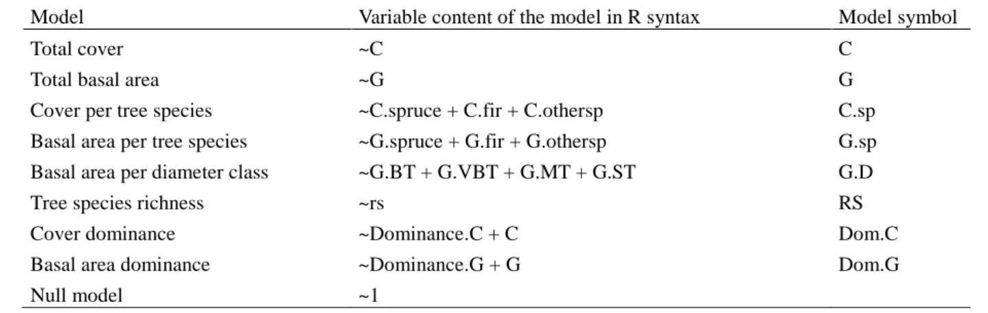
based on tree abundance (cf. Table 1). We added two points to this general objective: 287
whenever possible, we compared models based on cover data to similar models based on 288
basal area data (see below); and we added models which included the basal area of different 289
diameter classes. The latter addition was due to the inclusion of this work in a larger project 290
on tree stand simulators developed to test silvicultural scenarios which are mainly based on 291
diameter classes. Finally, we also added the interactions between the dendrometric models 292
and certain ecological gradients (see below). 293
The effect of both ecological variables and indicators on the species richness of the 294
different ecological groups was modeled through Bayesian models similar to Generalized 295
Additive Models (GAMs; Harrell, 2001). Since we were analyzing count data, the models we 296
used were mostly equivalent to Poisson GAMs, except that the Poisson distribution was 297
replaced by a more flexible distribution in the Bernoulli/Double Polya mixture-Poisson-298
Negative Binomial family – which allows for both under- and over-dispersion relative to the 299
Poisson distribution (Gosselin, 2011a; Gosselin, Unpublished). This meant that, conditional 300
on all the covariates, the variance of the model could be smaller or larger than the mean. The 301
link function was the classical logarithm link function for Poisson GAMs. 302
The ecological variables introduced into the model were: soil pH as indicated by the 303
Ellenberg values of the understory species (denoted as reaction), mean annual temperature 304
(T), growing season precipitation (PPT), solar radiation (solrad), topography, aspect and 305
slope. Temperature, reaction, precipitation and radiation were input into the model through an 306
automatic restricted cubic spline transformation involving four knots, thus requiring the 307
estimation of three parameters for each variable (Harrell, 2001). This transformation is 308
11
classical for species distribution models; it allows the function to model a possible non-linear 309
relationship between the transformed predictor and the explanatory variable. 310
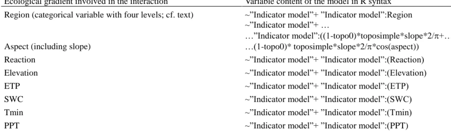
Topography was taken into account through a variable denoted as topo0 with a 1 311
value for flat positions and 0 otherwise (see Fig. SM1). This allowed us to model the 312
difference between flat topographies and the other topographies. Finally, aspect was taken into 313
account through a cosine function multiplied by a variable related to slope such that the 314
variable was equal to zero for zero slope (no aspect effect) and equal to 1 for slopes of 45° 315
and steeper. All these variables were put into the model as a linear combination of the 316
logarithm of the mean, The effect of the indicators we wanted to test (see Table 1) was added 317
to this linear combination either alone or in interaction with another ecological variable (see 318
Table 2). The formula for the logarithm of the mean, using a R-like syntax, was therefore: 319 " model Indicator " )) cos( * )) 4 / , ( pmin (sin( 0 ... ... ) 4 ), ( ( ) 4 ), ( ( ) 4 ), ( ( ) 4 ), ( (
topo I slope aspect
solrad scale rcs T scale rcs PPT scale rcs reaction scale rcs 320
where "rcs" is the R function for the restricted cubic spline transformation involving four 321
knots (Harrell, 2001), "I" is the identity link, "pmin" is the parallel minimum function (giving 322
the minimum value after comparing the elements of one or more vectors or matrices), "sin" 323
and "cos" are respectively the sine and cosine trigonometric functions. 324
Another parameter – related to the index of dispersion of the model – was also estimated as a 325
constant. The priors probability distributions of the fixed effects – i.e. the probability 326
distributions of the corresponding statistical parameters, before the data is taken into account 327
– were mostly weakly informative, often with a normal distribution of mean 0 and a standard 328
deviation of 2 as prior distributions. 329
This model structure was used throughout with variations only in the “Indicator model”, 330
which we now come to. The indicator models were either the models specified in Table 1 or 331
the models in Table 1 plus the interaction of this model with one of the ecological variables in 332
Table 2. As the ecological variable itself was often already present in the model, and to 333
compare models on similar grounds, the simple ecological effect itself was not included in the 334
model. The ecological variables investigated either corresponded to geographic regions as 335
advocated by Biggs et al. (2009), ecological variables related to ecological stress (especially 336
water stress) as studied by Michalet et al. (2002) and Callaway et al. (2002) (precipitation, 337
temperature, exposure,…) and soil pH, inspired from Tyler (1989). The aspect model 338
included a slope component because aspect effect was modulated by the value of the slope. 339
12
The simple models were then tested on the successional ecological groups 340
successively to determine for each group which indicators gave the best results. For each 341
ecological group, we then compared the best indicator model, first without interaction and 342
then in interaction with the ecological variables in Table 2.We selected four ecological 343
variables that involved the best models for further analyses (see Results section). 344
The Bayesian models were fitted through an adaptation of the algorithm proposed by Vrugt et 345
al. (2009) based on four trajectories, and a thinning parameter of 50. The convergence of the 346
models was checked with the Rubin and Gelman Rhat quantity, below 1.1 (Gelman et al., 347
2004). After convergence was reached, we asked each model to estimate 2,000 values of the 348
parameters. 349
To compare our models with each other, we used a modified version of the DIC – 350
Deviance Information Criterion (Spiegelhalter et al., 2002) –, as discussed by Celeux et al. 351
(2006), which consists in calculating the reference Deviance not at the mean of the parameters 352
but at an estimate of its mode – which here corresponded to the set of parameters leading to 353
the highest posterior probability. Indeed, the classical version of the DIC yielded incoherent, 354
unstable results with negative values for the number of parameters, a problem that the mode-355
based DIC did not have. 356
357
2.3.2 Analysis of model results 358
For each model, the direction and magnitude of the effects of the indicator parameters were 359
analyzed with the same methods as in Barbier et al. (2009a). For each indicator parameter we 360
studied the effect on the mean fitted value for species richness of an increase in the ecological 361
parameter of around one standard deviation. We chose the following increases for the 362
different parameters: 10 m².ha-1 for most basal area parameters (5 m².ha-1 for G.othersp and 363
G.ST, respectively basal area of species other than fir or spruce and basal area of stems less 364
than 17.5 cm in dbh), 15% for all tree crown cover parameters, except 7.5% for C.othersp, 1.5 365
genera for tree species richness and 0.2 for tree species dominance. For each parameter, we 366
reported the mean value of the log of the multiplier of the mean corresponding to such a 367
variation, its 95% confidence interval, and the probability of the significance test that the 368
parameter was null. Levels of statistical significance for parameters were symbolized as 369
follows: ** = p < 0.01 and * = p < 0.05. Inspired from Dixon and Pechmann (2005), we also 370
did an analysis based on equivalence and inequivalence tests to detect negligible effects: 371
based on Bayesian parameter estimations as in Camp et al. (2008), the aim of this analysis 372
13
was to identify (i) when the parameter has a high probability of being in an interval, called the 373
negligible interval, that is a priori considered to represent negligible effects, (ii) when the 374
parameter had a high probability of being below this interval and (iii) when the parameter had 375
a high probability of being above it. Two negligible intervals were distinguished: one for 376
weak negligibility and one for strong negligibility. We denoted by 0 < b1 < b2 the levels
377
associated to the two negligible intervals. We used the symbol 0 to describes cases where P(-378
b2 < log(β) < b2) ≥ 0.95 and 00 for the more stringent: P(-b1 < log(β) < b1) ≥ 0.95. Similarly,
379
we denoted by "-" cases where P(log(β) < -b1) ≥ 0.95 and "--" cases where P(log(β) < -b2) ≥
380
0.95 . These cases correspond to non-negligible negative and strongly non-negligible negative 381
effects, respectively. We had similar notations - "+" and "++" - for the positive side. We chose 382
b1 = 0.1 and b2 = 0.2 for species richness data, corresponding respectively to a multiplication
383
of species richness by exp(0.1) ≈ 1.11 and exp(0.2) ≈ 1.22 at the upper side of the negligible 384
interval. 385
386
We addressed our two main predictions by using a mixture of analyses based on 387
models comparison and the analysis of the magnitude of the effects of the models. Our first 388
prediction was that dendrometric models involving only tree abundance would be more robust 389
than those with either tree species richness or stand dominance. Our analyses relied on two 390
forms of evidence, both for dendrometric models without interaction with other ecological 391
variables and those with interaction either with aspect, altitude, reaction or region, which were 392
the most active variables among those tested (listed in Table 3; cf. Results section): 393
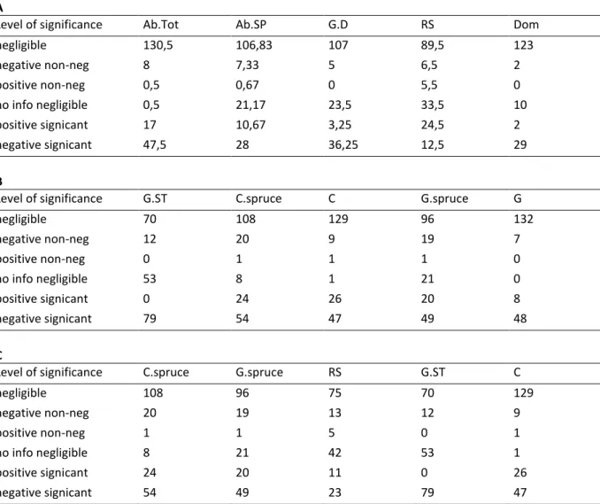
(i) model comparisons: for each category of dendrometric model (between Total Abundance, 394
Abundance by tree species, Abundance by diameter class, Tree species richness and Tree 395
dominance and abundance), either based on crown cover or on basal area, we recorded the 396
number of times the category of model was the best, the second best, and so on. We also 397
recorded the mean difference in DIC with the best model, over the 16 ecological groups 398
studied. A model that had less difference in DIC and a higher rank was interpreted as being a 399
better model than the others; 400
(ii) magnitude and significance of the effects: for each dendrometric parameter among the 401
floristic ecological groups, we recorded the number of times it was negative and significant to 402
the 1% level, positive and significant to the 1% level, judged negligible, negative non 403
negligible, positive non negligible or without enough information relative to negligibility of 404
the effect. These parameters were grouped in the same categories as in (i) above, except that 405
14
we also identified parameters for pure abundance (i.e. total abundance based either on crown 406
cover or basal area). 407
Our second prediction stated that dendrometric indicators would have relationships 408
with biodiversity that would depend on the ecological context. To tackle this prediction, 409
having selected the best four ecological variables (reaction, altitude, exposure and region; cf. 410
below), we compared the difference in DIC between the best model with interaction and the 411
best model without interaction. When the DIC value for the model with interaction was lower 412
by at least 5 DIC units from the model without an interaction, we interpreted this as an 413
indication of an interaction with the ecological gradient. 414
We then analyzed the magnitude of the effect of the dendrometric parameters on floristic 415
diversity in different ecological contexts to interpret the direction of this interaction. To do 416
this, for each dendrometric parameter we listed the ecological groups and ecological contexts 417
in which the relationship between the dendrometric parameter and the species richness of the 418
ecological group was judged negative non-negligible or positive non-negligible (cf. above). 419
For each dendrometric parameter, we also identified the ecological groups that were still 420
significantly negative non-negligible or positive non-negligible after the multi-comparison 421
correction proposed by Rice (1989). The estimators were taken at flat positions and at slope = 422
50% and aspects East or West, South and North aspect for aspect/slope models, and as the 423
mean+1*sd and mean-1*sd for elevation and reaction gradients. 424
To more collectively analyze the dependence of the indicator-biodiversity relationship on the 425
ecological context, we calculated the mean and standard deviation across ecological groups of 426
the difference at both ends of the ecological gradient in the mean effect of a typical variation 427
of the indicator on the log of the mean species richness. The differences taken were the 428
difference between South and North aspect at slope = 50% for aspect/slope models and as the 429
mean+2*sd and mean-2*sd for elevation and reaction gradients. 430
Finally, we checked the statistical quality of our models by using the new goodness of fit p-431
values proposed by Gosselin (2011b), called the sampled posterior p-values. We applied these 432
p-values on different aspects of normalized residuals (as described in Gosselin, 2011b): their 433
skewness, their kurtosis – to diagnose the probability distribution used -, their correlation with 434
the estimated mean – to diagnose general linearity problems – and with the covariates 435
incorporated in the models (precipitation, solar radiation, reaction, temperature…). To detect 436
potentially non-monotonous correlations between variables, we used the Hoeffding’s D 437
statistic provided in the Hmisc R package (Harrell, 2001). We applied this method to the best 438
model of each ecological group. We also checked the multi-collinearity of our variables of 439
15
interest by calculating the variance inflation factor (VIF) of all the dendrometric variables we 440
were interested in as a function of all the other variables in the model (Zuur et al., 2010). 441 442 3. Results 443 3.1 Choice of model 444
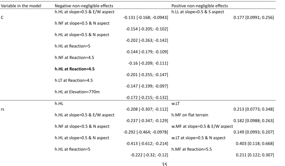
To determine which ecological gradients to include in interactions with our 445
dendrometric models, the simple models were first tested on the successional ecological 446
groups to determine which indicators gave the best results (Table SM.7). These indicators 447
were then run with the ecological variables in interaction as indicated in Table 2. Table SM.8 448
gives the results of this first comparison. The best models were: the "region:G.D" model for 449
mature forest and peri-forest herbaceous species, the "region:G.sp" model for non-forest 450
herbaceous species, the "region:RS" model for mature forest woody species and the 451
"reaction:G.sp" model for peri-forest woody species. Altogether, the aspect, elevation, 452
reaction and region variables performed best (see Table SM.8). 453
Furthermore, the goodness-of-fit checks of the best models of each group revealed 454
some significant departures from the probabilistic hypotheses in the models for more than half 455
of the ecological groups (9 over 16; Table SM.9). These departures involved the probability 456
distribution for species richness (4 cases) – indicating a problem in the probability distribution 457
used for these ecological groups –, the log link function (4 cases) or the relationships with 458
some ecological variables (8 cases in total) – indicating that more complex relationships 459
might be warranted for these groups. 460
Finally, regarding multicolinearity, some dendrometric variables in the simple models 461
had mildly problematic levels of VIF between 2 and 3 for the cover of spruce and fir (C.fir 462
and C.spruce) and for the total cover and dominance based on cover (C and Dominance.C) in 463
the Cover dominance model. For the first two, the problem was not strongly exacerbated in 464
the models with interaction. The other dendrometric variables had non problematic VIF 465
values below 2 (Zuur et al., 2010). 466
467
3.2 Prediction 1: dendrometric models based on abundance (i.e. basal area and tree cover) are 468
better than those based on dominance or tree species richness 469
Dendrometric models formulated on abundance data were better models overall than those 470
based on tree species richness (Table 3 and Tables SM3 to SM6). Indeed, the abundance-471
based models (i.e. G.sp and C.sp in Ab.SP and G.D) were the best for one third of the 472
16
biodiversity ecological groups on average whereas the species richness model (RS) was the 473
best for at most one sixth of the ecological groups. Furthermore, for the RS model, the mean 474
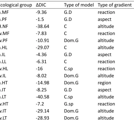
difference in DIC from the DIC of the best model ranged from 40% to more than 150% more 475
than for models based on abundance. Dom models (including Dom.C and Dom.G) involving 476
both tree species dominance and total tree species abundance were intermediate but rarely 477
provided the best model. 478
However, analysis of the significance and magnitude of the effects of the parameters in these 479
different models tempered the above results. Indeed, overall, the parameters in the tree species 480
richness models had the highest chance of involving a non-negligible relationship, whatever 481
the context (Table 4). Moreover, this result was not due to abundance parameters involving 482
more cases where there was not enough information to conclude. Rather the reverse was true. 483
The result was tempered for statistically significant results: the best variables were those 484
based on absolute abundance in the tree stand. Furthermore, when only herbaceous floristic 485
biodiversity was analyzed, leaving aside woody ecological groups, tree species richness 486
models were slightly surpassed by abundance models, by tree species or by diameter class for 487
the mean of significant results, although they still involved the most non-negligible 488
relationships on average (cf. Table 5). Also, for the five dendrometric variables that involved 489
the greatest number of significant results or the most number of non-negligible results, 490
dendrometric variables involving abundance data (total abundance, spruce abundance or 491
abundance of trees less than 17.5cm dbh) appeared among the first (cf. Tables 4 & 5). Tree 492
species richness was still a good dendrometric variable. Overall, tree species richness had 493
more positive than negative significant or non-negligible effects for woody floristic ecological 494
groups, but the reverse was true when the analysis was restricted to herbaceous ecological 495
groups (compare Tables 4 & 5). Variables related to tree abundance had mostly negative 496
effects on floristic biodiversity (see Table 4). 497
498
3.3 Prediction 2 : : dendrometric indicators have relationships with biodiversity that depend 499
on the ecological context: 500
An interaction between dendrometric variables and ecological context was detected for most 501
of the ecological groups (cf. Table 6). Only two ecological groups (peri-forest herbaceous 502
species and intermediate lightdemanding woody species) had DIC differences of more than -503
5 between the best interaction model and the best simple model, while five ecological groups 504
(non-forest herbaceous species, heliophilous herbaceous species, cold-temperature herbaceous 505
17
species, mid-temperature woody species and high-temperature woody species) had a DIC 506
difference of less than -20. 507
Regarding the ecological groups and contexts in which each dendrometric variable was a non-508
negligible indicator of biodiversity (cf. Table 7), most ecological groups were indicated in 509
specific ecological contexts, as hypothesized. Only in a few cases did dendrometric indicators 510
indicate a non-negligible variation across all the plots analyzed (2 for C.spruce, 1 for G.ST, 1 511
for G.spruce, 2 for rs and 1 for Dominance.G). Indicators related to tree abundance mostly 512
negatively impacted non-forest, high-light or low-temperature herbaceous species, mostly in 513
northern aspects, at lower elevations and in more acidic conditions. We noticed a counter 514
relationship of a positive non-negligible effect of some tree abundance attributes on south 515
facing slopes for low-light herbaceous species. We also noticed a positive effect of the basal 516
area of tree species other than spruce and fir on four ecological groups in the Internal Alps 517
(results not shown). Spruce cover and basal area as well as the basal area of trees less than 518
17.5 cm in dbh (G.ST) were the most involved in relationships with biodiversity. 519
The picture was somewhat different for tree species richness indicators: they mostly had 520
positive non-negligible effects on the species richness of herbaceous and woody forest species 521
as well as low-temperature woody species. Tree species richness had noticeable negative 522
effects on some herbaceous species groups, mostly for groups and in ecological conditions for 523
which there was also a negative impact of tree abundance indicators. 524
In addition, stand dominance based on basal area had a negative effect on low-temperature 525
woody species in many ecological contexts and on forest herbaceous species in two ecological 526
contexts. 527
528
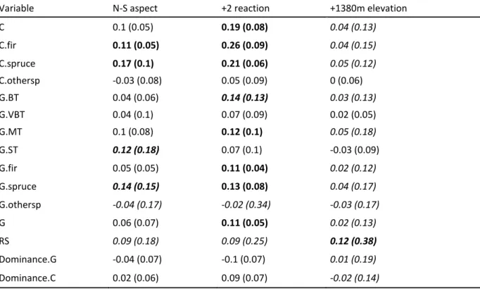
Finally, by analyzing the variation across ecological groups of their response to each 529
dendrometric ecological indicator along ecological gradients (cf. Table 8), we detected 530
unilateral variations in biodiversity in response to total cover, fir cover and spruce cover along 531
the reaction and aspect gradients. Slightly less strong results were detected for equivalent 532
basal area data as well as for the basal area of trees between 17.5 and 42.5 dbh. A slight 533
reverse trend was found for tree species richness based on cover for the aspect gradient and 534
for tree species dominance for the reaction gradient. Another, “variational” response, where 535
there was no strong central trend and considerable variation among ecological groups, was 536
detected for most cases along the elevation gradient as well as for some other cases along the 537
aspect and reaction gradients, especially for tree species richness. This means that while some 538
18
species groups had a response to the indicator that increased rather strongly along the 539
gradient, other species groups decreased strongly. 540
541
4. Discussion 542
4.1 Identifying the best dendrometric indicators of floristic variables 543
Our first prediction was that models involving tree abundance could account for variations in 544
floristic species richness better than models involving either tree species richness or 545
dominance. At the statistical model level, our prediction was met. This was not completely the 546
case at the individual predictor level, where variables in abundance models were on average 547
associated with fewer non-negligible effects than tree species richness variables. Finally, the 548
two best abundance variables, basal area of the smallest diameter class and spruce cover, 549
competed well with tree species richness in terms of non-negligible or significant results. Our 550
results are therefore less clear-cut than Barbier et al. (2009a) where the analyses based on 551
model comparisons and magnitude of the effects clearly converged. Nonetheless, our results 552
support considering models based on tree abundance as indicators of floristic biodiversity, as 553
suggested by many previous studies (Moir, 1966, McCune and Antos, 1981, Specht and 554
Morgan, 1981, Pitkanen, 2000, Brosofske et al., 2001, Ohlemüller et al., 2004, Laughlin et al., 555
2005, Lindh, 2005, references in Barbier 2009 and Vockenhuber et al., 2011). Our results also 556
suggest, however, that tree species richness may be a good univariate indicator of biodiversity 557
for some ecological groups, in accordance with previous results in the literature (Auclair and 558
Goff, 1971, Hicks, 1980, Ingerpuu et al., 2003, Vockenhuber et al., 2011 and references in 559
Barbier et al., 2008). 560
We are unsure at this stage why spruce abundance and small diameter tree abundance are 561
better indicators than the abundance of other tree species or diameter classes. Spruce 562
abundance performance in our study is all the more surprising that Mitchell and Kirby (1989), 563
when summarizing the literature, listed spruce and fir as having similar effects on floristic 564
species composition. This is not what we have found, although we did not analyze species 565
composition directly nor did we analyze the effect of spruce stand dominance, but rather the 566
effect of spruce abundance. It should be noted that spruce abundance and small diameter tree 567
abundance indicated – mostly negatively – partly different ecological groups (peri-forest 568
herbaceous species for small diameter tree abundance, heliophilous herbaceous species for 569
spruce abundance). 570
19
Multivariate models such as ours should be further studied to determine whether they are 571
better than univariate models of abundance or than univariate models involving the relative 572
abundance of some tree species, a commonly used variable in forest ecology (Ewald, 2000, 573
Mölder et al., 2008). We promote using absolute abundance rather than relative abundance 574
because it is more directly linked with ecological mechanisms, even though it has yet to be 575
confirmed as a better indicator. In any case, we advise testing abundance-based as well as 576
diversity-based dendrometric quantities as biodiversity indicators. 577
578
4.2 The relationship between dendrometric indicators and floristic biodiversity depends on the 579
ecological group and the ecological context 580
Our second prediction was rather general; it stated that the relationship between dendrometric 581
indicators and floristic biodiversity should depend on the ecological context. This prediction 582
was inspired firstly by general considerations as well as more specific results that point in this 583
direction (cf. Introduction section): most ecological relationships are not likely to be general 584
across all ecological conditions but instead should depend on the ecological context. Our 585
results partially confirmed our second prediction: the best models always included an 586
interaction of dendrometric indicators with an ecological gradient (cf. Table 6). The 587
relationships between individual indicators and the biodiversity of specific ecological groups 588
were more often non-negligible in certain specific locations (Northern slopes and Jura for 589
abundance models; Jura, Northern Alps, Internal Alps for RS). However, overall, though the 590
frequency of non-negligible cases was less frequent in simple models (2.9% of all groups, 591
3.7% for herbaceous groups only) than in models analyzed in specific ecological contexts 592
(3.7% of all groups, 5.4% for herbaceous groups only), the differences between these 593
frequencies were non-significant. This result means that even if we demonstrated the 594
importance of ecological context in the dendrometric indicator – biodiversity relationship, this 595
importance is somewhat relative. 596
597
4.3 Analysis of biodiversity relationships with indicators along gradients 598
In addition to studying the relationship between dendrometric indicators and floristic species 599
richness in specific ecological conditions, we also used a rather novel type of analysis to study 600
how these relationships vary among species groups along ecological gradients (cf. Table 8). 601
This analysis allowed us to characterize cases where the indicator/biodiversity relationship 602
20
was relatively stable across groups along the ecological gradient, but only in relative terms, 603
i.e. in terms of the differences between the coefficients of the indicators between groups. In 604
other words, there was a parallel shift of the relationship across groups along the gradient 605
(bold cases in Table 8). This is similar to a null model in which different ecological groups 606
respond differentially to an indicator, but with a difference in coefficients that remains 607
constant along the gradient. This was the case for indicators based on spruce and fir crown 608
cover measurements along the aspect and reaction gradients. These results could be translated 609
in ecological terms as a global shift from negative interactions between canopy abundance 610
and floristic biodiversity to more positive interactions from one side of the gradient to the 611
other. 612
In other cases, not only was the relative difference between estimators constant along the 613
gradient, but the estimators themselves were relatively constant in absolute terms. This 614
indicates that the relationship was stable between the indicator and biodiversity along the 615
gradient. For example, this was the case for the basal area of very large trees or the crown 616
cover of trees other than spruce and fir along the elevation gradient. 617
A third interesting case appeared where there was no central tendency in the variation in the 618
indicator/biodiversity relationship among ecological groups along the gradient but instead a 619
strong variance among ecological groups along the gradient (italic cases in Table 8). This 620
occurred for most of the indicators along the elevation gradient as well as for some indicators 621
along the aspect and reaction gradients. In this case, the indicator could very well be related to 622
biodiversity in some regions of the ecological gradient, but the biodiversity/indicator 623
relationship was unstable across ecological groups in relative terms along the ecological 624
gradient. 625
626
4.4 Two contrasted gradients for the relationship between tree abundance indicators and 627
herbaceous groups: aspect and soil reaction gradients 628
Following other authors, Austin and Van Niela (2011) made the point that species distribution 629
models should incorporate topographic variables to better predict the future distribution of 630
species in response to climate change. Our results on floristic biodiversity in forests are along 631
the same lines but we go a step further: our results indicate that not only should we take into 632
account topographic information, we should also take into account tree abundance and the 633
interaction between tree abundance and topographic variables. Our results indicate that denser 634
tree cover would decrease some floristic stand-level diversity in northern aspects while it 635
21
would promote other components of floristic diversity in southern aspects. This can be 636
interpreted in terms of the stress/facilitation hypothesis which states that positive interactions 637
between species are more likely in more ecologically stressful conditions (Callaway et al., 638
2002, Callaway, 1997, Michalet et al., 2002). Indeed, if we had used the Index of Moisture 639
Availability (IMA) as did Laughlin et al. (2005, based on Batek et al., 1999), our aspect 640
gradient would have been transformed into a water stress gradient since the IMA predicts 641
greater water stress on steep south-facing slopes. However, other mechanisms may become 642
limiting at certain points along the aspect gradient (e.g. light on northern aspects when tree 643
abundance is high and light levels are reduced). Therefore, we should not too hastily explain 644
the effect of such an indirect ecological gradient, in our case aspect, by a unique more direct 645
ecological gradient (see also Soliveres et al., 2011). 646
Michalet et al. (2002) observed that floristic species composition differed in fir and spruce 647
stands in the French Alps on southern aspects but not on northern aspects. This seems to be a 648
result qualitatively similar to ours in that it indicates an interaction of tree species effect on 649
biodiversity along the aspect gradient. However, in our study, the species richness response of 650
the ecological groups to fir abundance did not strongly differ from their response to spruce 651
abundance along the aspect gradient. Therefore, our results are not completely in agreement 652
with those of Michalet et al. (2002). One difference between Michalet et al. (2002)’s study 653
and ours is that we investigated the impact of tree species abundance, and not tree species 654
dominance in the stand. Also, while Michalet et al. studied species composition, we analyzed 655
the species richness of ecological groups, which reflects presence-absence species 656
composition only if the species inside each ecological group have homogeneous ecological 657
behaviors. 658
Similar observations were made on the soil reaction gradient – indicative of soil pH. 659
Here too, there was an opposite effect at each end of the gradient. The effects of tree 660
abundance on the species richness of many ecological groups were mostly negative in more 661
acidic conditions, while they were more positive in less acidic conditions (cf.Table 8 & Tables 662
SM.35 to SM.40). Ecologically interpreting this case in terms of stress is more difficult 663
because soil pH should indicate stress at both ends of the gradient, where two different 664
resources are involved (water and nutrients; Maestre et al., 2009). This should result in 665
positive effects of tree abundance at both ends of the gradient, unless the stress-gradient 666
hypothesis is refined as indicated by Maestre et al. (2009). Still our results appear to be in the 667
opposite direction to those of Tyler (1989), who documented a more negative effect of tree 668
crown cover on floristic diversity in less acidic conditions than in more acidic conditions. 669
22
Similarly, we did not confirm the stress-facilitation hypothesis along the altitudinal gradient as 670
did Callaway et al. (2002) (cf. Table 8 & Tables SM.28 to SM.33). Our results therefore 671
indicate that the “classic” stress-facilitation hypothesis appears on some gradients (here the 672
aspect gradient) but not on others (elevation and reaction) for the species richness of 673
ecological groups. This finding must still be verified through the analysis of the ecological 674
group abundance and species abundance. 675
676
4.5 Implications for forest management and biodiversity indicators 677
Of course, as for many observational ecological results, our results should be checked with 678
other observational data, other methods of analysis and with experimental data before they 679
can be applied with confidence in management. For example, we did not integrate all the 680
interesting ecological groups nor did we analyze abundance data. Our study was also limited 681
because we considered only one broad taxonomic group (understory vascular plant), which is 682
not necessarily indicative of all forest biodiversity. Work should be pursued in these directions 683
and our results should therefore not be unduly generalized. 684
Should our results be confirmed, we could say that variables such as spruce abundance, small 685
diameter tree basal area and tree species richness have a non-negligible relationship with the 686
species richness of relatively numerous floristic ecological groups. The relationships we 687
found were mostly negative for spruce abundance and small diameter tree abundance but can 688
be both negative and positive for tree species richness. Secondly, some of the abundance 689
parameters had interactions with some of the ecological gradients that were in the same 690
direction for the different ecological groups. This resulted, for example, in effects that 691
globally changed from negative to positive from northern aspects to southern aspects 692
(respectively, from acidic conditions to less acidic conditions) for the abundance of spruce 693
trees (respectively, spruce basal area and cover, fir cover, and basal area of big trees). This 694
means that if floristic biodiversity is the objective, managers should apply opposite guidelines 695
in these contrasted ecological conditions. 696
697
Our results support our initial prediction (cf. also Barbier et al., 2008, Barbier et al., 2009a) 698
which states that biodiversity indicators only reflect a part of the biodiversity in specific 699
ecological conditions. Our work therefore promotes evaluating biodiversity indicators to 700
specify in which ecological contexts and for which component of biodiversity the indicator 701
has a non-negligible relationship and whether the relationship is positive or negative. 702
703
23
Acknowledgements. This work was supported by the French Ministry of Agriculture through 704
grant n° E 23/2010 and FP7-KBBE project "ARANGE" (n° 289437). We thank Benoît 705
Courbaud, Thomas Cordonnier and Valentine Lafond for comments on dendrometric 706
indicators for silvicultural models. Patrick Vallet and Maude Toigo provided useful help on 707
the NFI database. We thank Vincent Boulanger (ONF) and two anonymous reviewers for their 708
help in improving the manuscript. We thank Vicki Moore for correcting the English. 709
710 711
References:
712
Auclair, A. N. and F. G. Goff, 1971. Diversity relations of upland forests in the western Great 713
Lakes area. The American Naturalist, 105(946), 499-528. 714
Austin, M. P. and K. P. Van Niel, 2011a. Impact of landscape predictors on climate change 715
modelling of species distributions: A case study with Eucalyptus fastigata in southern New 716
South Wales, Australia. Journal of Biogeography, 38(1), 9-19. 717
Austin, M. P. and K. P. Van Niel, 2011b. Improving species distribution models for climate 718
change studies: Variable selection and scale. Journal of Biogeography, 38(1), 1-8. 719
Austin, M. P. and T. M. Smith, 1989. A new model for the continuum concept. Vegetatio, 720
83(1-2), 35-47. 721
Barbier, S., 2007. Influence de la diversité, de la composition et de l'abondance des essences 722
forestières sur la diversité floristique des forêts tempérées. Ph.D thesis Thesis, Université 723
d'Orléans, Orléans. 724
Barbier, S., F. Gosselin and P. Balandier, 2008. Influence of tree species on understory 725
vegetation diversity and mechanisms involved - a critical review for temperate and boreal 726
forests. Forest Ecology and Management, 254(1), 1-15. 727
Barbier, S., R. Chevalier, P. Loussot, L. Bergès and F. Gosselin, 2009a. Improving 728
biodiversity indicators of sustainable forest management: tree genus abundance rather than 729
tree genus richness and dominance for understory vegetation in French lowland oak hornbeam 730
forests. Forest Ecology and Management, 258( ), S176-S186. 731
Barbier, S., P. Balandier and F. Gosselin, 2009b. Influence of several tree traits on rainfall 732
partitioning in temperate and boreal forests: a review. Annals of Forest Science, 66(602). 733
24
Batek, M. J., A. J. Rebertus, W. A. Schroeder, T. L. Haithcoat, E. Compas et al., 1999. 734
Reconstruction of early nineteenth-century vegetation and fire regimes in the Missouri 735
Ozarks. Journal of Biogeography, 26(2), 397-412. 736
Bertness, M. D. and R. Callaway, 1994. Positive interactions in communities. Trends in 737
Ecology and Evolution, 9(5), 187-191. 738
Biggs, R., S. R. Carpenter and W. A. Brock, 2009. Spurious certainty: How ignoring 739
measurement error and environmental heterogeneity may contribute to environmental 740
controversies. BioScience, 59(1), 65-76. 741
Brosofske, K. D., J. Chen and T. R. Crow, 2001. Understory vegetation and site factors: 742
implications for a managed Wisconsin landscape. Forest Ecology and Management, 146(1-3), 743
75-87. 744
Brown, M. J. and G. G. Parker, 1994. Canopy light transmittance in a chronosequence of 745
mixed-species deciduous forests. Canadian Journal of Forest Research, 24(8), 1694-1703. 746
Callaway, R. M., 1997. Positive interactions in plant communities and the individualistic-747
continuum concept. Oecologia, 112(2), 143-149. 748
Callaway, R. M., R. W. Brooker, P. Choler, Z. Kikvidze, C. J. Lortie et al., 2002. Positive 749
interactions among alpine plants increase with stress. Nature, 417(6891), 844-848. 750
Camp, R. J., N. E. Seavy, P. M. Gorresen and M. H. Reynolds, 2008. A statistical test to show 751
negligible trend: Comment. Ecology, 89(5), 1469-1472. 752
Cavaignac, S., 2009. Les sylvoécorégions (SER) de France métropolitaine, Etude de 753
définition, French National Forest Inventory, Nogent sur Vernisson. 754
Celeux, G., F. Forbesy, C. P. Robertz and D. M. Titteringtonx, 2006. Deviance information 755
criteria for missing data models. Bayesian Analysis, 1(4), 651-674. 756
Dixon, P. M. and J. H. K. Pechmann, 2005. A statistical test to show negligible trend. 757
Ecology, 86(7), 1751-1756. 758
25
Douguédroit, A. and M. F. de Saintignon, 1970. Méthode d'étude de la décroissance des 759
températures en montagne de latitude moyenne: Exemple des alpes françaises du sud. Revue 760
de géographie alpine, 58, 453-472. 761
Duelli, Peter and Martin K. Obrist, 2003. Biodiversity indicators: the choice of values and 762
measures. Agriculture, Ecosystems & Environment, 2063, 1-12. 763
Dufour-Kowalski, S., B. Courbaud, P. Dreyfus, C. Meredieu and F. De Coligny, 2012. 764
Capsis: An open software framework and community for forest growth modelling. Annals of 765
Forest Science, 69(2), 221-233. 766
Ellenberg, H., H. E. Weber, R. Düll, V. Wirth, W. Werner et al., 1992, Zeigerwerte von 767
Pflanzen in Mitteleuropa, vol. 18 (). Verlag Goltze, Göttingen. 768
Ewald, J., 2000. The partial influence of Norway spruce stands on understorey vegetation in 769
montane forests of the Bavarian Alps. Mountain Research and Development, 20(4), 364-371. 770
Gelman, A., J. B. Carlin, H. S. Stern and D. B. Rubin, 2004, Bayesian Data Analysis (). 771
Chapman & Hall, Boca Raton. 772
Glenn-Lewin, D. C., 1977. Species diversity in North American temperate forests. Vegetatio, 773
33, 153-162. 774
Gosselin, F., 2011a. Propositions pour améliorer l'équipement biométrique du détective 775
écologique. Application à la modélisation de la relation entregestion forestière et biodiversité. 776
HDR Thesis, Université Pierre et Marie Curie, Paris. 777
Gosselin, F., 2011b. A New Calibrated Bayesian Internal Goodness-of-Fit Method: Sampled 778
Posterior p-values as Simple and General p-values that Allow Double Use of the Data. Plos 779
One, 6(3), e14770. 780
Gosselin, F., 2012. Improving Approaches to the Analysis of Functional and Taxonomic 781
Biotic Homogenization: beyond Mean Specialization. Journal of Ecology, 100(6), 1289-1295. 782
Harrell, F. E., 2001, Regression Modeling Strategies, With Applications to Linear Models, 783
Logistic Regression, and Survival Analysis. Springer, New York, USA. 784