HAL Id: hal-00329396
https://hal.archives-ouvertes.fr/hal-00329396
Submitted on 3 Jun 2005
HAL is a multi-disciplinary open access
archive for the deposit and dissemination of
sci-entific research documents, whether they are
pub-lished or not. The documents may come from
teaching and research institutions in France or
abroad, or from public or private research centers.
L’archive ouverte pluridisciplinaire HAL, est
destinée au dépôt et à la diffusion de documents
scientifiques de niveau recherche, publiés ou non,
émanant des établissements d’enseignement et de
recherche français ou étrangers, des laboratoires
publics ou privés.
Low-latitude ionospheric turbulence observed by
Aureol-3 satellite
Y. Hobara, François Lefeuvre, Michel Parrot, O. A. Molchanov
To cite this version:
Y. Hobara, François Lefeuvre, Michel Parrot, O. A. Molchanov. Low-latitude ionospheric turbulence
observed by Aureol-3 satellite. Annales Geophysicae, European Geosciences Union, 2005, 23 (4),
pp.1259-1270. �hal-00329396�
Annales Geophysicae, 23, 1259–1270, 2005 SRef-ID: 1432-0576/ag/2005-23-1259 © European Geosciences Union 2005
Annales
Geophysicae
Low-latitude ionospheric turbulence observed by Aureol-3 satellite
Y. Hobara1,*, F. Lefeuvre1, M. Parrot1, and O. A. Molchanov2
1LPCE/CNRS, 3A, Avenue de la Recherche Scientifique, 45071, Orl´eans cedex 2, France
2United Institute of Physics of the Earth, RAS, 123995, Bolshaya Gruzinskaya 10, Moscow D-242, Russia *now at: Swedish Institute of Space Physics, Box 812, SE-981 28 Kiruna, Sweden
Received: 26 May 2003 – Revised: 1 March 2005 – Accepted: 14 March 2005 – Published: 3 June 2005
Abstract. Using PSD (Power Spectral Density) data on
elec-tron density and electric field variations observed on board Aureol-3 satellite at low-to-mid-latitude ionosphere we an-alyze a scale distribution of the ionospheric turbulence in a form k−α, where k is the wave number and α is the spectral index. At first, high-resolution data in the near-equator re-gion for several orbits have been processed. In this case the frequency range is from 6 Hz to 100 Hz (corresponding spa-tial scales from 80 m to 1.3 km), each power spectrum obeys a single power law fairly well, and the mean spectral indices are rather stable with αN=2.2±0.3 and αE=1.8±0.2, for the
density and electric field, respectively. Then we produce a statistical study of 96 electric field bursts in the frequency range 10–100 Hz from low-time resolution data (filter bank envelope). These bursts concentrate on the side of the Equa-torial Anomaly crest (geomagnetic latitude 30–40◦). Spec-tral indices of the bursts vary in the interval αE=2.0–2.5 but
are fairly stable in seasons and local times. The electric field power of the burst has rather a large variability but has a rel-ative increase in mean values for the summer and winter, as well as the daytime. The effect of major seismic activities to-ward the ionospheric turbulence is not conclusive either for the refractive index or for the electric field power. However, the mean value for the electric field power of bursts during seismic periods is larger than that for non seismic periods, and the statistical difference of the mean values is rather sig-nificant.
Keywords. Ionosphere (Equatorial ionosphere; Ionospheric
irregurlarities) – History of Geophysics (Seismology)
1 Introduction
Electron density irregularities in the low-latitude ionosphere (so-called Equatorial spread-F, ESF) were observed on the ground using either conventional ionosphere sounding or by recording of incoherent radar scattering signals or by scin-tillation technique. Spatial spectrum (or wave number spec-Correspondence to: Y. Hobara
(yasu@irf.se)
trum) of the irregularities vary from large scale with length L=20 km to short scale with L=0.1–10 m (Kelley, 1989). In-situ measurements on board satellites and rockets have given a great contribution to the present understanding of the ionosphere dynamics. Recent analysis of plasma den-sity measurements made aboard the AE-E satellite at alti-tudes above 350 km and below 300 km (Kil and Heelis, 1998) has revealed the existence of longitudinal variations due to F-region dynamics. The effect is seen most dramatically in the suppression of occurrence probabilities at altitudes above 350 km in longitude regions where interhemispheric winds in the magnetic meridian are the largest.
There were probe measurements of electrostatic potential fluctuations at wavelengths from a few meters to a few kilo-meters in the low-latitude ionosphere. In particular, vector electric fields in the frequency range f from 10 to 500 Hz have been measured on the 400 km altitude polar orbit-ing OV1–17 satellite (Kelley and Mozer, 1972), and Holtet et al. (1977) demonstrated the association between spread-F properties and electrostatic noise near lower hybrid fre-quency (fLH R∼10–15 kHz). Recently, Aggson et al. (1996)
presented electric field data from the San Marco D spacecraft in terms of structure and dynamics of ionospheric plasma (between 500 km and 800 km) depletions associated with night side equatorial spread-F. They measured two DC elec-tric field components in the zonal flow, westward and east-ward, and found bifurcations of these depletions.
Rather useful information on multi-scale near-equatorial spread-F turbulence was obtained from frequency spectra of electron density and electric field fluctuations observed on rockets (see, for example, the review by Kelley, 1989). It is usually supposed that the frequency spectrum, which is recorded on a moving platform with velocity V0, represents k-distribution in the form ω0=2πf0∼kV0(it is the so-called Taylor hypothesis), where f0 is the observed frequency of the variations and k is their wave number along the direction of the movement. Thus, the power spectrum density in the conventional form ∼(f0)−α is converted in the spatial dis-tribution ∼k−α with the same spectral index α. Jahn and LaBelle (1998) have recently presented the first rocket mea-surements of the ESF irregularities at altitudes above 600 km.
1260 Y. Hobara et al.: Low latitude ionospheric turbulence Power spectra of electron density fluctuations shows
dual-power law behavior with αNindices changed from αN≈1.7
at frequencies below 60 Hz to αN=5 at higher frequencies.
The electric field fluctuations in their experiment had spec-tral indices αE ranging from 3 to 4. A useful discussion
re-lated to the distinction between horizontal spectra observed along satellite tracks and the vertical wave number spectra measured with a rocket trajectory, further to the unified the-ory of observed density spectra, either by satellite or rocket, are found in the work by Kelley et al. (1987).
The same approach was used for some satellite data han-dling. Cerisier et al. (1985) analyzed electron density and electric field variations on board the Aureol-3 satellite in the frequency range 30–1000 Hz (scales L∼10–300 m). They found α=1.7–1.9 for the distribution of both parameters. However, they only analyzed one case at h∼600 km and at rather high magnetic latitude 8∼63◦. Molchanov et
al. (2002b) showed the connection between burst position of electric field variations at frequencies 10 kHz and 15 kHz (L∼0.5–0.8 m) and the Equatorial Anomaly (EA) depletion from observations performed with the satellite IK-24, and found αE=3–4. They revealed two regions of short-scale
electric field ionospheric turbulence near the equator and near the pole-ward gradient of the EA (invariant latitudes 20– 35◦), and demonstrated that the intensity of the turbulence increased during several cases of seismic activity. In their re-cent paper, Molchanov et al. (2004b) analyzed, in addition, large-scale (L=15–300 km) low-latitude density turbulence using Cosmos-900 data and reported αN values in a range
1.3–2.0. They found a statistical decrease of the turbulence intensity in association with seismicity. Distinction of spec-tra between the source altitude of the ionospheric turbulence (low altitude) and satellite altitude (high altitude) where the observation is made is reported by many papers (e.g. Hysell et al., 1994). We are going to produce similar research with Aureol-3 data but with middle spatial scale, low-altitude, and low-to-middle latitudes, which are not covered by the previ-ous works from Cosmos-900 and IK-24.
2 Data
The low-altitude Aureol-3 satellite was launched on 21 September 1981. The satellite is three-axis stabilized with the Z axis close to vertical and has a nearly polar orbit with a perigee at 400 km and an apogee at 2000 km. Based on the primary objectives, we use the data from electron den-sity measurement and electric field measurement. The elec-tron density is measured by the high-resolution Interferome-ter Self-Oscillating Probe (ISOPROBE) experiment (B´eghin et al., 1982), with a time resolution of 0.2 ms.
The horizontal AC electric field component (EH) used
in this study is obtained from the Tr`es Basses Fr´equences (TBF) experiment (Berthelier et al., 1982). Definition of the coordinate system of the satellite is as follows: X axis is the direction of the nominal velocity vector, Z axis is ver-tical to the spacecraft, and Y is perpendicular to either the
Xof the Y axes. The horizontal electric field (EH) is
mea-sured by pairs of spherical sensors located at the end of in-sulated booms (making angles of 11.5◦and 18◦with the YZ
and XY planes, respectively) and the distance between sen-sors for the EH component is 7.87 m. High time
resolu-tion waveforms in the frequency range from 1 Hz to 1500 Hz with a 5 kHz sampling rate are transmitted to the ground, while the data from 6 band-pass filters with frequency range of 10 Hz−20 Hz, 20 Hz−45 Hz, 45 Hz−100 Hz, 100 Hz−200 Hz, 200 Hz−450 Hz, and 450 Hz−1000 Hz are recorded in a magnetic tape on board the satellite. For time resolution of sampled values for each filter, 1t depends on the so-called ZAP of the Soviet telemetry mode and it ranges from ZAP1 (1t=0.01 s) to ZAP4 (1t=2.56 s). Dy-namic range of the observed signal is 60 dB.
High time resolution data with the simultaneous record-ing of electron density and electric field are available only near the telemetry stations and we use these for a case study around the KOUROU telemetry station (5.2◦N, 52.8◦W) to investigate equatorial ionosphere. On the other hand, elec-tric field data from filter banks (FB) can be sampled over the entire Earth, in spite of their poor time and frequency resolu-tions, and they are suitable for a statistical study.
3 Results and discussion
3.1 Case study (high time resolution data)
We use 5 different equatorial passes of the Aureol-3 satellite over the KOUROU telemetry station in June 1982. These passes were chosen for the previous work by B´eghin et al. (1985) in relation to the plasma density irregularities, in association with the ESF, because the satellite has a perigee near the magnetic equator at local times between 20 and 22. Altitudes for those passes range from 400 km to 550 km.
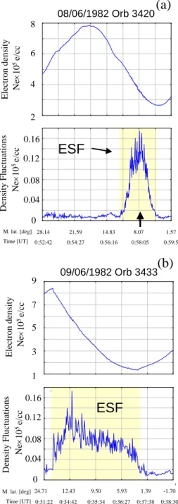
Figures 1a and b show the electron density profiles (top panels) and relevant RMS density fluctuations (bottom pan-els) for 8 and 9 June, respectively. Due to the telemetry limi-tation, the data for the Southern Hemisphere are not obtained, however a significant increase in density fluctuation in the northern edge of the density depletion is identified, which is thought to be associated with Ionospheric Turbulence (IT) within the ESF. The spread in magnetic latitude of turbulence varies between 8 and 15 deg in these examples. The other 3 passes have a similar tendency for the location and size of the irregularities (not shown).
In the equatorial region, spectral analysis of the Aureol-3 data is performed for the electron density fluctuation or for the horizontal electric field inside IT. Considering the same time resolution between the electric field and the electron density data (0.2 ms), the Fast Fourier Transform is applied to obtain the Power Spectral Density (PSD) by using a 900-point window with 8-time averaging process, hence we pro-duce one PSD profile about each second. In Fig. 2 we present an example of electron density and electric field spectra in-side IT at 0:58:10.43 UT at the altitude of 437 km during the
Y. Hobara et al.: Low latitude ionospheric turbulence 1261 Density Fluctuations Electron density Ne ×1 0 5e/ cc Electron density Density Fluctuations
Figure 1
2 3 4 5 6 7 8 100 150 200 250 300 350 400 450 500 0 0.02 0.04 0.06 0.08 0.1 0.12 0.14 0.16 0.18 100 150 200 250 300 350 400 450 500 M. lat. [deg]ESF
08/06/1982 Orb 3420(a)
.
.
28.14 21.59 14.83 8.07 1.57.
.
0 0.02 0.04 0.06 0.08 0.1 0.12 0.14 0.16 0.18 150 200 250 300 350 400 1 2 3 4 5 6 7 8 9 150 200 250 300 350 400ESF
09/06/1982 Orb 3433(b)
.
24.71 12.43 9.50 5.93 1.39 -1.70.
.
1 3 5 7 9 2 4 6 8 0 0.04 0.08 0.12 0.16 0 0.04 0.08 0.12 0.16 M. lat. [deg] 0:52:42 0:54:27 0:56:16 0:58:05 0:59:50Time [UT] Time [UT] 0:31:22 0:34:42 0:35:34 0:36:27 0:37:38 0:38:30
Ne ×1 0 5e/ cc Ne ×1 0 5e/ cc Ne ×1 0 5e/ cc Density Fluctuations Electron density Ne ×10 5e/ cc Electron density Density Fluctuations
Figure 1
2 3 4 5 6 7 8 100 150 200 250 300 350 400 450 500 0 0.02 0.04 0.06 0.08 0.1 0.12 0.14 0.16 0.18 100 150 200 250 300 350 400 450 500 M. lat. [deg]ESF
08/06/1982 Orb 3420(a)
.
.
28.14 21.59 14.83 8.07 1.57.
.
0 0.02 0.04 0.06 0.08 0.1 0.12 0.14 0.16 0.18 150 200 250 300 350 400 1 2 3 4 5 6 7 8 9 150 200 250 300 350 400ESF
09/06/1982 Orb 3433(b)
.
24.71 12.43 9.50 5.93 1.39 -1.70.
.
1 3 5 7 9 2 4 6 8 0 0.04 0.08 0.12 0.16 0 0.04 0.08 0.12 0.16 M. lat. [deg] 0:52:42 0:54:27 0:56:16 0:58:05 0:59:50Time [UT] Time [UT] 0:31:22 0:34:42 0:35:34 0:36:27 0:37:38 0:38:30
Ne ×10 5e/ cc Ne ×1 0 5e/ cc Ne ×1 0 5e/ cc
Fig. 1. Latitudinal variations (geomagnetic latitude) of the electron density along the Aureol-3 equatorial pass for two different days (top panels) and relevant RMS amplitude normalized by ambient electron density indicating the density fluctuations (bottom panels). Time in UT is also indicated along with geomagnetic latitude. The arrow in (a) indicates the time when the power spectral density in Fig. 2 is taken.
8 June pass. The arrow in Fig. 1a indicates the time of the above mentioned spectrum for the electron density fluctua-tion taken inside the ESF.
The density and electric field spectra obey a power law fairly well in the frequency range 6∼100 Hz (lower portion of the frequencies in the figure). This frequency range corre-sponds to the spatial scale from 80 m to 1.3 km by assuming
Figure 2
(a)
(b)
L [m] 800 80 8 L [m] 800 80 8α
n
~2.0
α
E
~2.2
EH
Ne
Electric fi eld power (m V/m ) 2Hz -1Power density (dNe/Ne)
2Hz
-1
08/06/1982/ 0:58:10.043 (UT) Mlat=7.81 deg, Alt=437.0 km
Figure 2
(a)
(b)
L [m] 800 80 8 L [m] 800 80 8α
n
~2.0
α
E
~2.2
EH
Ne
Electric fi eld power (m V/m ) 2Hz -1Power density (dNe/Ne)
2Hz
-1
08/06/1982/ 0:58:10.043 (UT) Mlat=7.81 deg, Alt=437.0 km
Fig. 2. Power spectra of the electron density (a) and horizontal electric field fluctuations, (b) inside the ionospheric turbulence (IT) to be associated with the ESF observed by the Aureol-3 satellite during the 8 June pass.
that the group velocity of irregularity is significantly smaller than the satellite velocity ∼8 km/s. For this long wavelength, Eand δN e/N e have a same frequency or k-dependence. The spectral indices of electric and density fluctuations α defined by PSD ∝f−αare equal to about 2. LaBelle et al. (1986) ob-tained the spectral density of about 2.5, both for electron den-sity and electric field fluctuations for the spatial scale larger than 100 m at the altitude of 450 km by the rocket measure-ment. The spectral index they measure (∼2.5) is larger than the value that we measure (∼2). On the other hand, the
1262 Y. Hobara et al.: Low latitude ionospheric turbulence
Figure 3
3 (6Hz<f<100Hz) 2.5 1 1.5 2 Spectral indexNe
EH
0.5 0June 2 June 3 June 8 June 9 June 10
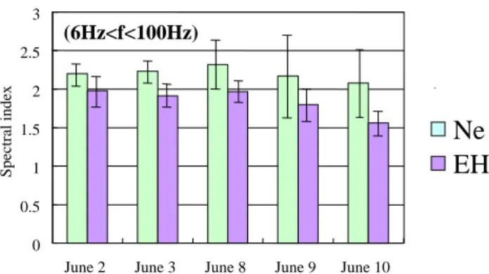
Fig. 3. Average spectral indices of the electron density (white) and electric field (shadowed) fluctuations inside the ESF for 5 different nights (20∼22 LT) for the frequency from 6 Hz to 100 Hz. Error bars indicate the relevant standard deviations.
proportionality between δE and δNe/Ne is obtained during
our measurement, as LaBelle et al. (1986) observed. It indi-cates that the Rayleigh-Taylor instability regime may work in theory (LaBelle et al., 1986). However, the observed spectral index varies from different rocket measurements. Kelley et al. (2002) show the power law spectra with the indices 1.92 and 1.72 for the electron density and the electric field, respec-tively, for the spatial scale larger than 100 m at the altitude 350 km, which are smaller than the index value we measure. Jahn and LaBelle (1998) reported the spectral index for elec-tron density fluctuation as 1.7 and from 3 to 4 for the electric field fluctuation below 60 Hz (large spatial scale) at the al-titude higher than 600 km. Kelley et al. (1987) reported the difference in the spectral index of electron density fluctua-tion between satellite and rocket measurements. This differ-ence in the spectral index may be due to the differdiffer-ence in the horizontal (satellite) cuts through spread F turbulence versus vertical (rocket). In addition, the anisotropy in the electric field turbulence makes it very difficult to compare the power laws derived from different electric wave field components.
At a shorter spatial wavelength (from 8 m to 80 m), both spectra have clear characteristic breaks at the spatial scale around 80 m (100 Hz), and several peaks are recognized for the electric field and density spectra. It is then difficult to derive a spectral index behind those peaks. According to the previous report, using the waveform data from the Aureol 3, the peaks observed on the EH power spectrum in the
fre-quency range 400–500 Hz in Fig. 1 correspond to the lower frequency cutoff of whistler waves (Lefeuvre et al., 1992). These peaks occupy a rather large area of the high frequency range. Therefore, we do not take into account this high fre-quency part and we will only consider the lower frefre-quency part up to 100 Hz.
Mean values of spectral indices for 5 different equatorial passes are shown in Fig. 3. Again, the linear least-squares fit to the power spectra from each data window was performed by the selected spatial scale range (6 Hz to 100 Hz) in relation to the break in the spectra around 80 m. The mean spectral index for density fluctuations is in a range from 2.08 to 2.32,
while the mean slope value for the electric field is always smaller than that for density (from 1.56 to 1.98). The day-to-day difference of the mean spectral index may not be very large (mostly δα∼0.2), and a positive correlation in the slope value between the electric field and density can be identified. The size of the error bars indicating the standard deviation of the spectral index within ESF may show the variability of the individual ESF event characteristics observed along the satellite trajectory. Taking into account the mean and the variability of the density and electric field fluctuations, we may conclude that the differences between the spectral in-dices for these two different physical parameters are in the range of error in the same pass.
3.2 Statistical study (filter bank data)
The horizontal electric field signals at six filter channels ob-served by the Aureol-3 satellite enable us to derive the power spectrum. These low-time resolution filter bank (FB) data are obtained over the entire Earth, in contrast to the data from high-time resolution density and electric field wave-forms transmitted only around the telemetry stations that we have chosen for the case study. Therefore, we can use the FB data for the statistical study to derive the characteristics of the IT for low-to-mid latitudes during the mission operations over a period of 4 years or more.
Two main drawbacks for the analysis of the FB data in this telemetry mode are (1) no relevant electron density spec-tra, (2) a relatively low sensitivity of the electric field. Is-sue (1) concerns how we can derive the characteristics of IT from the electric field component. In our case study, a rather good correlation between the electric field and den-sity fluctuation spectra has been found at the topside F re-gion in the latitude ionosphere inside IT for the low-frequency range. Cerisier et al. (1985) reported that the spec-tral indices between density and horizontal electric field fluc-tuations are nearly identical within experimental errors in the high-latitude ionosphere by using high-time resolution Aureol-3 data. Hence, it is reasonable to assume that the spectral index for IT is identical to that obtained from the horizontal electric field for the first 3 low-frequency channels of the FB (f<100 Hz, the frequency allocation is described in Sect. 2). The typical latitudinal variation of the electric field power for the first 3 FB channels in the low-to-mid latitude range (Figs. 4c and d) barely exceeds the instrument noise level of the FB, represented by a flat line attributed to the low sensitivity of this equipment. To obtain a meaningful spec-tral index, we use the part of the electric field power of which the intensity is significantly larger than this background noise level, to be defined as a burst event.
The burst event is a structure with a remarkable increase in the electric field power along the vehicle trajectory that is identified by its intensity and orbital limitations. We use the following criteria for the burst identification: (1) The electric field power (f<100 Hz), using PSD integrated over 3 first FB channels, must be higher than the upper quartile plus 1.5 times the inter quartile range from the corresponding
Y. Hobara et al.: Low latitude ionospheric turbulence 1263
Figure 4(a)
Orbit 1
Burst
Orbit 2
(a)
Figure 4(b)
Burst
Orbit 3
(b)
Figure 4(c)
Mlat [deg] Glong[deg] Altitude [km] Time [UT] -15.09 0.06 19.95 40.95 148.98 149.88 151.43 154.52 879.06 717.04 544.85 433.11 09:20:24 09:24:19 09:29:24 09:34:341982/03/12 Orbit 2
Electric fi eld power(c)
Figure 4(d)
1982/02/04 Orbit 3
-40.00 -19.96 0.09 20.06 40.16 142.04 140.62 139.33 137.77 135.29 619.94 492.05 415.46 404.94 457.57 02:15:51 02:11:25 02:06:48 02:02:15 01:57:51 Mlat [deg] Glong[deg] Altitude [km] Time [UT] Electric fi eld power(d)
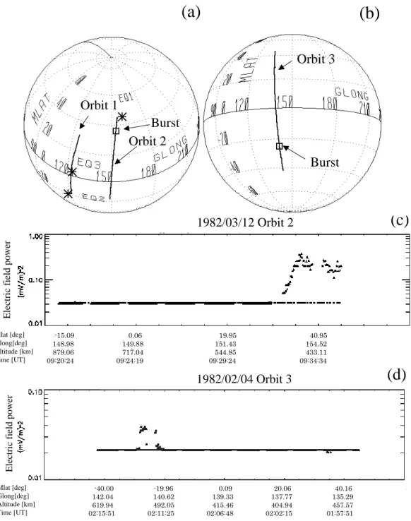
Fig. 4. Examples of satellite orbits and observed burst events in the electric field. (a) Two satellite orbits (orbit 1 and 2) on 12 March 1982 and major seismic events near the orbits are marked by an asterisk (*), while the approximate location of the burst event in the trajectory is marked by a square. (b) Same format as (a) for the orbit 3 on 4 February 1982 but no major earthquake is detected and the burst is observed. (c) Horizontal electric field power variation along the orbit 2 shown in (a). The intensive burst observed around 35◦N in the magnetic latitude with major earthquake nearby. (d) Same format as (c) but the burst event without major earthquakes. Orbit 1 has two major earthquakes nearby but no burst is observed.
half orbits. This threshold value is generally used to find ex-treme values, (2) the time duration of the observed burst must be longer than 12.8 s, which corresponds to ∼100 km in the minimum spatial scale at the low altitude. The burst is then fairly well captured above this threshold because most of the time the energy level is around the instrument noise level, ex-cept for the burst part indicating that the probability
distribu-tion of the energy in log scale does not obey a normal distri-bution. Furthermore, (3) spatial constraints (satellite altitude <900 km and −45◦<magnetic latitude <45◦) are applied to
limit the bursts related to the low-to-mid latitude IT, because intensive electrostatic turbulence is observed in association with the field-aligned density enhancement with ELF hiss in the high-latitude ionosphere (Cerisier et al., 1985). Applying
1264 Y. Hobara et al.: Low latitude ionospheric turbulence
Year Month Day Hour Min. Sec. Mlat. [deg] Glon. [deg] E power [dB] Spectral index Earthquake
1981 10 2 14 22 40 -15.3 171 2.46 2.31 X 1981 11 4 9 50 52 43.5 9.5 18.21 2.35 1981 11 4 22 35 19 34.4 176 11.82 2.63 X 1981 11 8 21 24 45 36.7 187.1 8.82 2.47 X 1981 11 8 23 16 10 42.9 161.3 7.54 3.03 X 1981 11 9 1 4 38 42.5 133 19.13 2.57 X 1981 11 9 2 53 17 42.6 104.9 16.72 2.81 1981 11 10 20 50 20 41.9 193.6 8.11 2.83 X 1981 11 11 22 20 10 32.7 167.6 11.96 2.16 1981 11 12 9 17 48 41.2 3.6 12.29 2.42 1981 11 24 16 35 45 42.7 231.5 2.4 2.47 1981 11 26 17 50 34 44.1 210.8 1.04 2.45 X 1981 12 22 18 11 54 -37.9 341.2 8.47 2.72 1981 12 22 21 55 54 -41.5 294.5 3.55 2.3 1981 12 23 1 30 14 -43.6 232.2 0.62 2.22 1981 12 24 13 53 49 -43.6 40.7 6.03 2.88 1981 12 24 21 18 45 -41.9 301.3 13.17 2.62 1982 1 5 11 52 47 -33.9 47.5 19.38 3.31 1982 1 13 22 13 46 -43.5 245.4 2.24 1.86 1982 1 13 23 59 4 -37 214.5 16.03 2.33 1982 1 19 12 55 55 -44.5 9.6 17.95 3 1982 1 20 21 46 53 -40.2 237.9 9.08 2.21 1982 1 20 23 33 28 -36.4 208.6 14.3 2.01 X 1982 1 21 1 22 3 -39.6 180.8 17.77 3.08 X 1982 1 21 3 9 21 -37 152.4 14.17 2.82 1982 1 21 10 26 36 -39.2 42.7 16.48 1.85 X 1982 1 21 12 16 49 -44.6 15.6 14.6 2.47 X 1982 1 22 1 3 17 -41.2 184.2 20.4 3.28 X 1982 1 22 2 50 36 -38.7 155.8 14.12 1.62 1982 1 22 11 57 26 -44.6 18.7 18.46 2.8 X 1982 1 23 20 48 19 -35.9 246.8 0.77 1.88 1982 1 23 22 36 52 -39.6 218.8 18.8 2.28 X 1982 1 24 0 23 32 -35.1 189.9 14.06 1.83 X 1982 1 24 2 13 16 -43.6 162.7 10.71 2.29 X 1982 1 25 21 58 31 -39.5 225.4 15.13 1.6 X 1982 1 25 23 45 47 -37.7 196.7 0.02 2.08 X 1982 1 26 10 38 26 -39.9 30.7 20.51 2.44 1982 1 26 21 39 58 -41.2 229.1 18.72 2.69 X 1982 1 27 21 20 50 -41.7 232.5 13.34 1.8 X 1982 1 27 23 7 58 -40.2 203.6 15.14 2.18 X 1982 1 28 0 53 59 -32.9 174.5 12.18 1.83 X 1982 1 28 2 40 44 -27 146.2 3 1.93 X 1982 1 28 11 52 14 -44.7 11 10.75 3.24 1982 1 30 0 16 28 -37.6 181.5 16.74 2.08 X 1982 1 30 16 48 28 -39.8 302.3 0.12 1.84 X 1982 1 31 23 39 20 -43.6 188.8 15.22 2.28 1982 2 1 1 26 46 -42.9 160.4 23.55 3.82 1982 2 2 23 0 23 -42.7 195.3 12.02 2.24 1982 2 3 0 47 47 -42 166.9 18.88 2.55 1982 2 3 2 32 8 -25 137.7 0.92 1.93 1982 2 3 6 13 50 -42.1 83.9 15.21 2.06 1982 2 3 20 50 3 -31.2 225.2 1.94 2 1982 2 4 2 13 2 -27.1 141.1 2.51 1.73 1982 2 24 9 31 22 43.5 183.3 8 2.1 X 1982 2 25 12 49 15 44.4 131.3 0.96 2.08 X
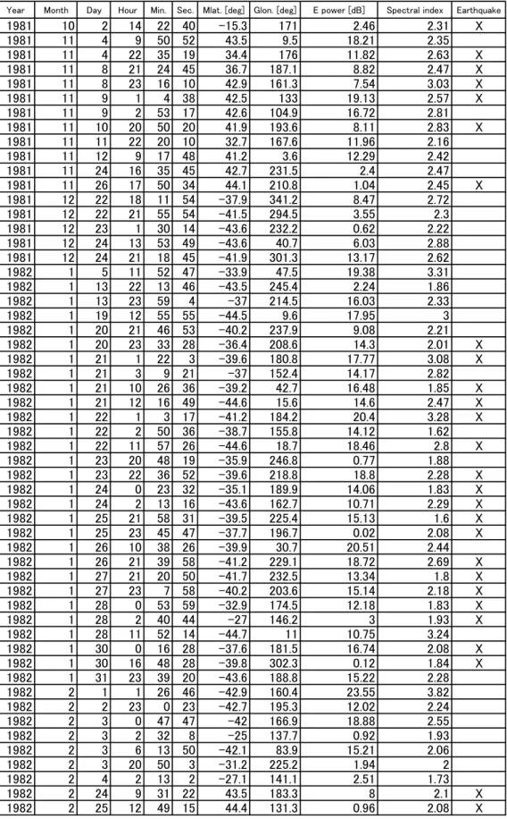
Table 1. List of electric field burst events and related parameters (year, date, time, magnetic latitude, geographic longitude, electric field power, spectral index, and earthquake) used in the statistical study. “X” in the column of the earthquake means that the burst is associated with the seismic activities and no “X” is for the burst without seismic activity.
Y. Hobara et al.: Low latitude ionospheric turbulence 1265 1982 2 26 12 29 20 44.5 134.8 9.97 2.75 X 1982 2 28 20 54 50 44 4.1 12.49 2.7 1982 3 12 9 33 29 36.5 153.6 10.31 2.76 X 1982 3 15 23 3 31 42.4 303.1 0.1 2.14 1982 3 16 0 51 38 42.7 275.1 18.72 2.62 1982 3 16 4 28 47 28 219.8 1.53 2.21 1982 3 17 0 29 19 34.9 277.8 10.42 2.77 1982 3 17 7 52 6 39.6 171.5 19.97 3.63 X 1982 3 18 0 7 46 30.8 280.9 9.74 2.37 1982 3 18 3 47 29 28 226.5 0.33 2.41 1982 3 18 20 15 44 44.1 342.8 9.61 2.11 1982 5 4 1 8 49 -44.6 12.1 8.06 2.74 1982 5 4 3 1 10 -43.6 349.8 17.88 0.86 X 1982 5 27 0 4 50 -40.5 347.9 17.65 2.18 1982 5 30 18 39 17 23.2 49.8 0.02 2.07 1982 6 2 19 36 38 -39.7 37.9 6.11 1.99 1982 6 4 20 41 0 -38.5 17.6 12.78 2.74 1982 6 4 22 34 50 -38.7 352.1 2.72 1.85 1982 6 6 9 5 55 -36.8 190.8 17.32 1.86 X 1982 7 26 4 31 59 42.1 356.4 4.68 1.84 1982 8 19 0 59 8 40.5 8.3 0.92 1.75 1982 9 29 23 8 43 -40.8 299.5 1.39 1.74 1982 10 17 10 11 35 36.3 297.1 6.93 -0.1 1982 12 10 3 11 26 43.8 142.2 12.4 2.99 1983 1 4 0 25 34 34.3 138.6 2.94 2.19 1983 1 7 17 16 59 24.2 235.7 0.12 2.56 1983 1 7 19 10 20 37 210.3 4.54 2 1983 2 14 15 42 41 -44.8 17.2 0.12 2.37 1983 3 10 15 1 49 -41.3 350.4 15.77 1.56 1983 3 10 16 48 19 -30.1 320.8 2.78 1.86 1983 4 6 21 55 10 -36.5 195.2 0.16 1.73 1983 4 19 10 21 22 43.6 171.1 2.07 2.48 1983 5 19 23 2 25 44.2 283.8 6.12 3.52 1983 5 23 23 8 50 41.9 275 12.61 2.6 1983 5 25 22 18 24 42.5 284.4 6.34 3.45 1983 9 7 6 28 6 31.4 343.2 0.03 2.21 1983 9 10 9 18 38 15.5 106.9 0.09 2.53 1983 9 10 12 24 59 43.3 248.4 2.95 2.98 1983 12 14 8 1 36 -37.8 335.9 14.94 2.7 1984 11 28 10 25 49 41.3 231.9 1.67 2.16 1985 3 25 20 45 36 41.6 234.4 15.46 2.02 Table 1. Continued.
this condition, we may exclude the bursts that have a high-latitude origin.
A total of 96 burst events are found after a careful ex-amination of each half-orbit cursory selected by the above-mentioned criteria. Basic parameters of burst events are sum-marized in Table 1. Periodical gaps in the data in the latitudi-nal variation of the electric field power in Figs. 4c and d are due to the internal calibration process of the instrument and they are removed from the original data. Bursts are seen in the wide latitudinal ranges, although they often occur in the mid-latitude side (20◦<absolute value of magnetic latitude <40◦) rather than the equatorial region, as it is seen in the two examples. Longitudinal locations of the bursts (Fig. 5) are rather uniformly distributed, except for a remarkable de-crease in the event numbers between 60◦to 120◦. This
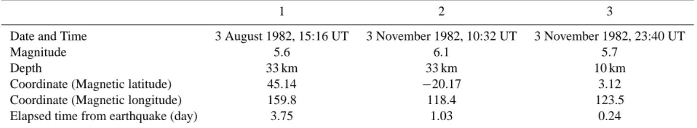
de-crease in the number of events is due to the reduced number of orbits at this location. We have generated the longitudi-nal distributions of the number of half orbits used and burst orbits among half orbits (not shown). As a result, there is a remarkable decrease (∼30% from mean value) in the number of available orbits in the longitude ranging from 60◦to 120◦. Figures 4a and b show the satellite trajectory in the magnetic latitude and geographic longitude coordinates. Locations of peak intensity of ionospheric bursts are marked by squares, and asterisks in Fig. 4a represent epicenters of major seismic events around the half orbits. The principal parameters of those seismic events are summarized in Table 2.
All seismic orbits used in the statistical study are cho-sen under the spatial and temporal conditions, which are: 1) M>5.5, 2) 1mlong<15◦ with ionospheric burst, and
1266 Y. Hobara et al.: Low latitude ionospheric turbulence
Table 2. Principal parameters of three seismic events (EQ 1 to EQ3) around the orbits 1 and 2 shown in Fig. 4a.
1 2 3
Date and Time 3 August 1982, 15:16 UT 3 November 1982, 10:32 UT 3 November 1982, 23:40 UT
Magnitude 5.6 6.1 5.7
Depth 33 km 33 km 10 km
Coordinate (Magnetic latitude) 45.14 −20.17 3.12
Coordinate (Magnetic longitude) 159.8 118.4 123.5
Elapsed time from earthquake (day) 3.75 1.03 0.24
Figure 5
-50 -40 -30 -20 -10 0 10 20 30 40 50 0 50 100 150 200 250 300 350Geographic longitude [deg]
Geomagnetic latitude [deg]
Fig. 5. Latitude-longitude distribution of the ELF electric field bursts (FB).
3) 1Day<5 days.
For the first condition, we use the CD-ROM of the seis-mic catalogue by NGDC (National Geophysical Data Center) which includes major seismic events from 1964 to 1995 cov-ering the period of our statistical analysis, and we extract all seismic events with a magnitude, M, larger than 5.5 and with a depth smaller than 100 km during the observation period of Aureol 3. The determination accuracy of an epicenter varies event by event, but it will be within a few degrees, which is much smaller than the spatial condition (2).
Secondly, in accordance with the condition (2), we define 1mlong as the difference of geomagnetic longitude between the epicenter and the satellite track. We examine each half orbit which contains the ionospheric burst and seismic event where the geomagnetic longitude of the epicenter is located at less than 15◦from the satellite track.
A third condition is related to the timing of the earthquake; the seismic events satisfying condition (2) should occur ±5 days (delay or precedence from the earthquake time) from the passage of the satellite.
Our timing and location criteria mentioned above are sim-ilar to the previous work for the ionospheric turbulence with seismic activity performed with the Intercosmos 24 satellite data (Molchanov et al., 2002b). Due to the limited num-ber of orbits with burst events during our observation period (totally 96 events), increasing the magnitude threshold de-creases significantly the number of burst orbits and
deterio-rates the accuracy of the statistical parameters, such as the mean value. On the other hand, decreasing the magnitude increases the number of seismic orbits but it is difficult to de-termine causative earthquakes (many earthquakes can satisfy the criteria for each half orbit). Our criteria are chosen to avoid the significant overlapping of the seismic events, either in space or in time coordinates.
Representative electric field power and relevant spectral index are calculated for each burst event. The field power is obtained by averaging the data points in largest intensity within 12.8 s, which corresponds to 5 data points for ZAP4. The associated spectral index is derived by the linear least-squares fit procedure using averaged values of the output from each FB channel up to 100 Hz (the frequency alloca-tion of the filter bank is given in Sect. 2).
Figures 6a and b are the bar graphs displaying the results from statistical analysis, including 96 burst events for spec-tral indices and burst intensities, respectively. The number at the top of each bar indicates the number of burst events included. The height of the bar represents the mean value calculated from the events in the bin. The confidence inter-vals with 95% for different bins, either for the spectral index or electric field power, are calculated based on the Gaussian distribution by using the mean value, standard deviation and number of samples for each group, which are indicated as er-ror bars in Fig. 6. One can find the method to calculate the confidence interval in Bendat and Piersol, 1971. The analy-sis for each parameter is performed for different seasons and local times. One year is separated by two groups of time peri-ods, which are spring (March to May) and autumn (Septem-ber to Novem(Septem-ber), and summer (June to August) and winter (December to February). Three different local time periods are examined: morning and evening (3 to 9 LT and 15 to 21 LT), day (9 to 15 LT), and night (21 to 3 LT). We also sep-arate the events between seismic (dark bars) and noseismic (white bars) orbits. Furthermore, since large geomagnetic activity can affect the generation of the AGW in the mid-dle latitude, we have examined the effect of the geomagnetic activity on the ionospheric bursts related to the earthquakes. The mean and standard deviation of sum Kp index are
cal-culated ±5 days from each ionospheric burst. Mean value of Kpis 22.6, with a standard deviation of 4.1 for the burst
with seismic events while the mean of 22.2 and a standard deviation of 5.4 are obtained for the bursts without seismic
Y. Hobara et al.: Low latitude ionospheric turbulence 1267
Table 3. The probability to have different parent distributions between seismic and non seismic periods corresponding to the groups in Figure 6(a) and 6(b).
Spring and Autumn Summer and Winter Morning and Evening Day Night All
Spectral index 0.55 0.67 0.55 0.05 0.5 0.094
Electric field power 0.7 0.82 0.61 0.38 0.45 0.93
0 0.5 1 1.5 2 2.5 3 3.5 64 32 29 10 35 22 26 4 28 23 10 5 0 4 8 12 16 20 Spring Autumn Summer Winter Morning Evening
Day Night All
Electric fi eld power [dB] 64 32 29 10 35 22 26 4 28 23 10 5 Spectral index
(a)
(b)
No EQs
With EQs
Fig. 6. Seasonal and local time dependence of the averaged (a) spectral index and (b) electric field power of the burst events. Shad-owed bins represent the bursts with major seismic activities and white bins are for the bursts without seismic activity. Error bars indicating the 95% confidence interval for each bin are calculated by using Gaussian distribution. Very large confidence intervals for groups (morning and evening, and nighttime) for seismic events are mainly due to the small number of events in the bin.
activity. According to the statistical test with the Gaussian distribution, the probability of having a statistical difference in the mean Kp value between the bursts with and without
earthquakes in our data set is 22%. Hence, the effect of Kp
on the seismic and non-seismic period is not significant. Sea-sonal and local time variations of the mean spectral index shown in Fig. 6a, together with error bars indicate that the indices are fairly stable α∼2.3 and the difference in values falls in the error range. For two cases with small event num-bers (4 events for morning or evening with seismic events, and 5 events for nighttime with seismic events), confidence intervals for these events are rather large (1.28 and 1.24, re-spectively) due mainly to the small number of events. In-dices between seismic and non-seismic events show neither a significant difference nor clear systematic dependence on seasons and LT, because the probabilities of having different
parent distributions for any sub-groups do not exceed 67% (Table 3). This leads to the remarkable similarity between the two indices shown in the upper right corner representing the average values grouped by all seismic and non-seismic events (The probability that the mean values belong to dif-ferent parent distributions is of ≈9% only). None of the 6 different pairs in Fig. 6a indicate the remarkable statistical difference of mean value. However, one should keep in mind that the EA starts after sunrise and vanishes after midnight, while ESF is predominantly observed in the nighttime pe-riod. The similarity in the index between different local time periods indicates that the ionospheric turbulence developing near the magnetic equator and the outer slope of the equa-torial anomaly crest has a similar physical nature, even if they have different primary seeding processes. Accordingly, a rather good consistency of the slope value may suggest that the similar type of generation mechanism may be connected to the observed bursts (then to the IT) for all seasons and LT. Moreover, the average value α∼2.3 falls in the range of the indices obtained for the IT inside the ESF in the case study and thus the contribution from the Rayleigh-Taylor instabil-ity in the long wavelength as a primary source might be an-ticipated for the observed burst events in the statistical study. In addition, the IT in the high altitude ionosphere can also be possible when the IT in the E-layer propagates upward by the transformation of atmospheric turbulence intensified by the tide, neutral wind, and severe weather conditions, etc.
As for the intensity variations (Fig. 6b), a rather large vari-ability in the electric field power of the bursts is revealed. The error bars representing the confidence interval are cal-culated by the same procedure taken for the spectral index (using a Gaussian distribution with a level of confidence of 0.05). The very large confidence interval for the event in two groups (morning and evening, and nighttime) is due to the small number of events in the bin. Except for these cases, relatively large variability may suggest that the burst inten-sity is highly variable between the cases in nature. Other several possible reasons to explain this large variability may exist. Firstly, the satellite may not pass through the region of maximum intensity because of the longitudinal separation of the orbits, which leads to an underestimation of the peak in-tensity. This effect also depends on the spatial scale of the burst. Secondly, the true distribution of the power might have a noticeable departure from the Gaussian distribution, and a simple standard deviation is not a suitable parameter to describe the variability. Indeed, the histograms shown in Fig. 7b may hint at the possible reason for this large
variabil-1268 Y. Hobara et al.: Low latitude ionospheric turbulence
Figure 7
(a)
(b)
Solid: ALL Dotted: EQ
Dash dotted: NO EQ Solid: ALL
Dotted: EQ Dash dotted: NO EQ
Figure 7
(a)
(b)
Solid: ALL Dotted: EQDash dotted: NO EQ Solid: ALL
Dotted: EQ Dash dotted: NO EQ
Fig. 7. Probability distributions of (a) spectral index and (b) elec-tric field power of the elecelec-tric field bursts. Solid lines represent all events, dotted lines are for bursts with major seismic activities, and dash dotted lines are for bursts without seismic activities.
ity. The distribution for the electric field power of bursts is derived by the same method and groups as that used for the spectral index (Fig. 7a). Note that the occurrence probabil-ity has two enhanced intensprobabil-ity ranges, (1) 0 dB to 5 dB and (2) 8 dB to 20 dB, and does not perfectly obey the Gaussian distribution for all three groups, which might lead to a large variance.
For any case, a much larger event number is necessary for an accurate determination of the distribution function. Thus, we found it difficult to statistically prove the difference in
the mean values between the different seasonal and local time conditions because of the overlapping of confidence intervals for the different groups. Nonetheless, if we use a smaller confidence for each bin, the following remarks can be made. First of all, a larger mean electric field power is found in association with a higher occurrence probability of bursts in the daytime in comparison with other local time periods. This tendency is opposed to the higher occurrence rate such as that in the ESF. However, a relatively large-scale density gradient structure and associated electric field can exist in the low to mid-latitude ionosphere in the dayside despite the rapid production and recombination rate such as the EA.
Second, the large intensity bursts are preferably observed in the northern summer and winter rather than in the spring and autumn. The difference in mean power is about 2 dB.
In relation to the seismic and non-seismic periods, the mean values for the seismic periods for any group are larger than those for the non-seismic periods (Fig. 6b), but one has to consider carefully the difference in mean values based on the statistics. The probability of having different mean val-ues between the seismic and non-seismic periods, based on the Gaussian distribution, was calculated for the electric field power of the bursts (Table 3). The probability for the elec-tric field burst is larger than that for the spectral index in any group. Among the sub-groups (seasons and LTs), the sum-mer and winter group has the largest probability (82%) of having a different mean value. Hence, none of sub-groups indicate a significant statistical difference (e.g. a confidence level larger than 90%), which means that the difference in the mean electric field power between the seismic and non-seismic events is not statistically proven for each season or LT. However, the group which contains all events (32 seis-mic events and 64 non-seisseis-mic events, shown in the right-hand side group in Fig. 6b) reveals a statistical difference in the mean value between the seismic and non-seismic events for the 93% confidence. The mean value of burst electric field power associated with the seismic events is larger than that without seismic activity by ∼4 dB in this case. The distribution of the occurrence probability of the burst elec-tric field power shown in Fig. 7b may support this tendency. The probability for the bursts associated with major seismic events increases for larger power (from 10 dB to 20 dB) and decreases for smaller power (from 0 dB to 8 dB), in compar-ison with the burst without major earthquakes. This large burst power related to seismic activity can be connected to the robust ionospheric turbulence.
Several effects linked to the seismic activity can contribute to the IT. The first are the emissions of aerosols (radioac-tive gas or metallic ions) which are well known before earth-quakes (see the review by Toutain and Baubron (1998) who listed various measurements of geochemical precursors in-cluding radon). The transportation to ionospheric layers is due to atmospheric turbulence and thermospheric winds. There is an increase of the atmosphere conductivity, a pen-etration of the electric fields and an ion acceleration. This leads to anomalous electric field generation, plasma instabil-ities, and the generation of waves at various frequencies
(Pu-Y. Hobara et al.: Low latitude ionospheric turbulence 1269 linets et al., 1994). The second effect is related to the ground
surface thermal anomalies (Tramutoli et al., 2001; Tronin, 2002; Tronin et al., 2002) which appear several days be-fore strong earthquakes in the earthquake preparation area, and the latent heat anomalies also discovered with the help of remote sensing techniques in the earthquake preparation zone (Dey and Singh, 2003). These two effects generate AGW whose effect may be important because as far as they propagate, the AGW amplitude increases due the decrease in the atmospheric density. They can trigger small-scale tur-bulence (E-field oscillations) due to plasma inhomogeneity (Molchanov et al., 2001, 2002a, 2004ab; Miyaki et al., 2002). Quantitative estimates of AGW initiation due to temperature variations observed both on the ground and from satellites (IR radiation) are reported by Molchanov (2004a).
4 Conclusions
The electron density and horizontal electric field data ob-served at high-altitude ionosphere by the Aureol-3 satellite have been analyzed to investigate the ionospheric turbulence with approximate frequency range 6 Hz to 100 Hz (spatial scales from 80 m to 1.3 km).
Simultaneous recording of high-time resolution waveform data, both for the density and electric field for successive days, allows us to investigate the temporal dependence of the power spectral density in the ionospheric turbulence within the ESF at the altitude range 400 km∼550 km. We ob-tained the following remarks: (1) In the low-frequency range (f <100 Hz), each power spectrum obeys fairly well a single power law, and the mean spectral indices are αN=2.2±0.3, αE=1.8±0.2 for the density and electric field, respectively.
These observed spectral indices fall in the range of the ones previously reported, (2) the similarity in index between the electron density and the electric field (αN and αE) implies
that the Rayleigh-Taylor instability regime might work in this long wavelength, as it was suggested in previous works, (3) observed spectral indices are rather stable and have a posi-tive correlation between density and electric field for differ-ent days. This suggests the fact that those two parameters are closely connected in relation to the relevant instability pro-cess.
Low-time resolution electric field data recorded over the entire Earth by the filter bank system are used to charac-terize the seasonal and local time dependence of the iono-spheric turbulence (IT) by assuming similar properties be-tween the density and electric field fluctuations seen in the case study. The averaged spectral index of the low frequency portion (f <100 Hz) for the 96 electric field events observed at low-to-mid latitudes are found to be stable and they do not depend on seasons and on local times. This indicates that the wave number spectra of the IT at the satellite altitude (>400 km) are nearly identical, even in the case where the primary seeding energy source and possible instability mech-anisms might be different. The averaged electric field power (f <100 Hz) of the ionospheric bursts has a large variability,
and the statistical difference of mean values between the dif-ferent seasons and LTs is not identified. However, relative increases in mean values for summer, winter and daytime are seen. According to the simple statistical test, the mean val-ues of spectral index between seismic and non seismic bursts are not statistically different (the probability of having dif-ferent parent distributions is smaller than 0.67). On the con-trary, the mean value of the electric field power for the seis-mic bursts is larger than that for non-seisseis-mic bursts with 93% confidence. This difference of mean values between seismic and non-seismic groups is statistically proven when all bursts are taken into account. However, the statistical differences for any sub-groups (different seasons and LTs) are not large (the probability of having different distributions is smaller than 0.8). Hence, the effect of seismic events on the electric field power of the ionospheric bursts is still inconclusive. For more accurate investigation, it is highly desirable to increase the number of burst events with the simultaneous recording of the density and electric field, together with the influence of major sources of IT rather than increasing seismic activi-ties, such as the tide, severe weather, and volcanic activiactivi-ties, which we did not take into account in this paper. The future low altitude satellite like DEMETER (Parrot, 2002) is one of the ideal missions to resolve this unclear issue.
Acknowledgements. This work is supported by ISSI (International
Space Science Institute) in Bern, Switzerland under the project 45. Authors would like to thank C. B´eghin and D. Lagoutte for the use-ful discussion and the CDPP (Centre de Donn´ees de la Physique des Plasmas) for the Aureol-3 data.
Topical Editor M. Lester thanks two referees for their help in evaluating this paper.
References
Aggson, T. L, Laakso, H., Maynard, N. C., and Pfaff, R. F.: In situ observations of bifurcations of equatorial bubbles, J. Geophys. Res., 101, 5125–5138, 1996.
B´eghin, C., Karczewski, J. F., Poirier, B., Debrie, R., and Masse-vich, N.: The ARCAD-3 ISOPROBE experiment for high time resolution thermal plasma measurements, Ann. Geophys., 38(5), 615–630, 1982.
B´eghin, C., Pandey, R., and Roux, D.: Instabilities associated with the equatorial spread-F phenomenon and their north-south asym-metry, in Results of the ARCAD 3 project and the recent pro-grams in magnetospheric and ionospheric physics, Ed. CNES, Publ. CEPADUES, Toulouse, 537–546, 1985.
Bendat, J. S. and Piersol, A. G.: RANDOM DATA: Analysis and Measurement Procedures, John Wiley and Sons, Inc., 1971. Berthelier, J. J., Lefeuvre, F., Mogilevsky, M. M., Molchanov, O.
A., Galperin, Y. I., Karczewski, J. F., Ney, R., Gogly, G., Guerin, C., Leveque, M., Moreau, J. M., and Sene, F. X.: Measurements of the VLF electric and magnetic components of waves and DC electric field on board the AUREOL-3 satellite: The TBF-ONCH experiment, Ann. Geophys., 38(5), 643–668, 1982.
Cerisier, J. C., Berthelier, J. J., and B´eghin, C.: Unstable density gradients in the high-latitude ionosphere, Radio Sci., 20, 755– 761, 1985.
1270 Y. Hobara et al.: Low latitude ionospheric turbulence
Dey, S. and Singh, R. P.: Surface latent heat flux as an earthquake precursor. Nat. Haz. Earth Syst. Sci., 3, 749–755, 2003. Holtet, J. A., Maynard, N. C., and Heppner, J. P.: Variational
electric fields at low latitudes and their relation to spread-F and plasma irregularities, J. Atmos. Terr. Phys., 39, 247–262, 1977. Hysell, D. L., Kelley, M. C., Swartz, W. E., Pfaff, R. F., and
Swen-son, C. M.: Steepened structures in equatorial spread-F-1. New observations, J. Geophys. Res., 99, 8827–8840, 1994.
Jahn, Jorg-Micha and LaBelle, J.: Rocket measurements of high-altitude spread F irregularities at the magnetic dip equator, J. Geophys. Res., 103, 23 427–23 441, 1998.
Kelley, M. C., and Mozer, F. S.: A satellite survey of vector electric fields in the ionosphere at frequencies of 10 to 500 Hz, 3, Low-frequency equatorial emissions and their relationship to iono-spheric turbulence, J. Geophys. Res., 77, 4183–4189, 1972. Kelley, M. C., Seyler, C. E., and Zargham, S.: Collisional
inter-change instability. II - A comparison of the numerical simula-tions with the in situ experimental data, J. Geophys. Res., 92, 10 089–10 094, 1987.
Kelley, M. C.: The Earth’s Ionosphere: Plasma Physics and Elec-trodynamics, Int. Geophys. Ser., 43, Academic Press, San Diego, Calif., 1989.
Kelley, M. C., Franz, T. L., and Prasad, G.: On the turbulent spectrum of equatorial spread F: A comparison between lab-oratory and space results, J. Geophys. Res., 107(A12), 1432, doi:10.1029/2002JA009398, 2002.
Kil, H. and Heelis, R. A.: Global distribution of density irregulari-ties in the equatorial ionosphere, J. Geophys. Res., 103, 407–417, 1998.
LaBelle, J., Kelley, M. C., and Seyler, C. E.: An analysis of the role of drift waves in equatorial spread-F, J. Geophys. Res., 91, 5513–5525, 1986.
Lefeuvre, F., Rauch, J. L., Lagoutte, D., Berthelier, J. J., and
Cerisier, J. C.: Propagation characteristics of dayside
low-altitude hiss - Case studies, J. Geophys. Res., 97, 10 601–10 620, 1992.
Miyaki, K., Hayakawa, M., and Molchanov, O. A.: The role of gravity waves in the lithosphere-ionosphere coupling, as revealed from the subionospheric LF propagation data, Seismo
Elec-tromagnetics: Lithosphere-Atmosphere-Ionosphere Coupling,
edited by: M. Hayakawa and Molchanov, O. A., TERRAPUB, Tokyo, 173–176, 2002.
Molchanov, O. A., Hayakawa, M., and Miyaki, K.: VLF/LF sound-ing of the lower ionosphere to study the role of atmospheric oscil-lations in the lithosphere-ionosphere coupling, Advances in Polar Upper Atmosphere Research, N15, 146–158, 2001.
Molchanov, O. A., Hayakawa, M., Afonin, V. V., Akentieva, O. A., and Mareev, E. A.: Possible influence of seismicity by grav-ity waves on ionospheric equatorial anomaly from data of IK-24 satellite 1. Search for idea of seismo-ionosphere coupling, Seismo Electromagnetics: Lithosphere-Atmosphere-Ionosphere Coupling, edited by: Hayakawa, M. and Molchanov, O. A., TER-RAPUB, Tokyo, 275–285, 2002a.
Molchanov, O. A., Hayakawa, M., Afonin, V. V., Akentieva, O. A., Mareev, E. A., and Trakhtengerts, V. Yu.: Possible influ-ence of seismicity by gravity waves on ionospheric equatorial anomaly from data of IK-24 satellite 2. Equatorial anomaly and small-scale ionospheric turbulence, edited by: Hayakawa,
M. and Molchanov, O. A. in: Seismo-Electromagnetics
(Lithosphere-Atmosphere-Ionosphere Coupling), TERRAPUB, 287–296, 2002b.
Molchanov O. A.: On the origin of low- and middle-latitude iono-spheric turbulence, Physics and Chemistry of the Earth, 29, 559– 567, 2004a.
Molchanov O. A., Akentieva, O. S., Afonin, V. V., Mareev, E. A., and Fedorov, E.: Plasma density-electric field turbulence in the low-latitude ionosphere from the observation on satellites; pos-sible connection with seismicity; Physics and Chemistry of the Earth, 29, 569–577, 2004b.
Parrot, M.: The micro-satellite DEMETER, J. of Geodynamics, 33, 535–541, 2002.
Pulinets, S. A., Legen’ka, A. D., and Alekseev, V. A.: Pre-earthquakes effects and their possible mechanisms. In: Dusty and Dirty Plasmas, Noise and Chaos in Space and in the Laboratory. Plenum Publishing, New York, 545–557, 1994.
Toutain, J. P. and Baubron, J. C.: Gas geochemistry and seismotec-tonics: a review. Tectonophysics, 304, 1–27, 1998.
Tramutoli, V., Di Bello, G., Pergola, N., and Piscitelli, S.: Robust satellite techniques for remote sensing of seismically active ar-eas. Annali de Geofisica, 44, 295–312, 2001.
Tronin, A. A.: Atmosphere-lithosphere coupling. Thermal anoma-lies on the Earth surface in seismic processes. In: Seismo-Electromagnetics: Lithosphere-Atmosphere – Ionosphere Cou-pling. Edited by: Hayakawa, M. and Molchanov, O. A., TER-RAPUB, Tokyo, 2002, 173–176, 2002.
Tronin, A. A., Hayakawa, M., and Molchanov, O. A.: Thermal IR satellite data application for earthquake research in Japan and China. J Geodyn., 33, 519–534, 2002.