Acoustic wood tomography on trees and the challenge
of wood heterogeneity
Sandy Schubert1,*, Daniel Gsell1, Jurg Dual2, Masoud Motavalli1and Peter Niemz2
1Empa, Du¨bendorf, Switzerland 2ETH Zu¨rich, Zu¨rich, Switzerland
*Corresponding author.
Empa, U¨ berlandstrasse 129, CH-8600 Du¨bendorf, Switzerland E-mail: sandy.schubert@empa.ch
Abstract
The assessment of tree stability requires information about the location and the geometry of fungal decay or of a cavity in the interior of the trunk. This work aims at specifying which size of decay or cavity can be detected non-destructively by acoustic wood tomography. In the present work, the elastic waves that propagate in a trunk during a tomographic measurement were visualized by numerical simulations. The numerical model enabled to systematically investigate the influence of fungal decay on tomographic measurements neglecting the hetero-geneity of wood. The influence of wood heterohetero-geneity was studied in laboratory experiments on trunks. The experiments indicated that the waveforms of the meas-ured signals are by far more sensitive to the natural het-erogeneity of trunk wood than the travel times, thereby making waveforms unsuitable for decay detection. Thus, it is recommended to further develop the travel time inversion algorithms for trunks and to neglect the infor-mation in waveforms or amplitudes. Fungal decay is detectable if the influence of the decay is distinguishable from the influence of the heterogeneity. It was found from the numerical analysis that the cross-section of a cavity, which is larger than 5% of the total cross-section of the trunk, can be detected by acoustic wood tomography.
Keywords: acoustic; assessment; decay; finite
differ-ence method; numerical simulation; tomography; trees; ultrasound.
Introduction
The failure of trees in an urban environment can endan-ger lives and damage infrastructure. The main aspects that determine the stability of a tree are: trunk diameter, weight- and wind-loading, strength of trunk wood, root anchorage as well as the location and geometry of fungal decay or a cavity in the interior of a stem. The assess-ment of the interior of a stem requires reliable testing methods. One approach is acoustic wood tomography (AWT), which consists of exciting elastic waves sequen-tially on several source positions, measuring the arrival of the fastest wave by circumferentially attached
receiv-ers and inverting the measured travel times using a mechanical model of the stem. Several studies (Nicolotti et al. 2003; Gilbert and Smiley 2004; Rabe et al. 2004) evaluated AWT by comparing tomograms with the real density distribution of the measured stems. The results in these quoted papers indicate that AWT is a promising approach for the detection of fungal decay. Socco et al. (2004) improved AWT by normalizing the results by a ref-erence plane. Maurer et al. (2006) eliminated systematic errors in the tomograms due to the isotropic trunk model by an anisotropy correction factor. However, the reliability of the method still has to be verified. In the present work, a systematic approach to evaluate AWT is used, which is based on the numerical simulation of the wave prop-agation phenomena in a stem and is supported by the experimental verification of the simulation model. This work aims at specifying which size of decay or cavity can be detected by AWT and is a first step of assessing the reliability of this testing method.
It is essential for further optimization of AWT to under-stand the wave propagation phenomena in the tree. Only very few studies investigated this phenomena. Bulleit and Falk (1985) calculated the P-wave arrival times in poles with and without decay with a 2D finite element model. Payton (2003) derived analytically the wave fronts of P-and the in-plane S-wave in the radial-tangential plane of wood. In their previous work, Schubert et al. (2006) simu-lated the wave propagation phenomenon in the radial-tangential plane of a trunk by the finite difference meth-od. The simulations visualized the differences in the shape of the wave fronts for a full and a hollow trunk. The different wave front shapes resulted in different travel times to the measurement points on the surface as well as a v- and a w-shaped curve of the average velocities for the full and the hollow trunk, respectively. However, a 3D simulation of the wave propagation in the tree, which is described in the present work, is necessary if not only travel times but also waveforms and amplitudes of the signals are interpreted.
In the present work, the curve shapes of the average velocities are verified by experiments. The aims of the experiments were: (1) to verify the results of the numer-ical simulations, and (2) to verify whether the waveforms of the measured signals contain additional information that can be used for improving AWT. Furthermore, the opportunities and limitations of AWT are demonstrated.
Materials and methods
Numerical simulation by a finite difference model The simulation model is an idealization and represents a stem with a circular cross-section, a pith in the center and a vanishing grain angle. The piths of trees are usually much weaker than the
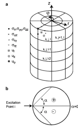
Figure 1 (a) The trunk model subdivided into grid cells and the coordinate system; for the grid cell (k, j, l), the positions of the displacement and stress components. (b) The relative position between the excitation point and the measurement point is described by the angle a.
surrounding wood and thus they were modeled by means of a small cylindrical hole in the center of the model. Material damp-ing and effects due to varydamp-ing material parameters were neglect-ed. The assumed orthotropic material behavior of the tree is described by the stiffness tensor C with its nine independent elastic moduli relating the stresses s and the strains ´:
ssCØ´ (1)
Since the orthotropic behavior of the trunk is cylindrical in nature, the equations of motions are formulated in cylindrical coordinates: 2 ≠ ur ≠srr 1 ≠srw ≠srz srr-sww r s q q q , 2 ≠t ≠r r ≠w ≠z r 2 ≠ uw ≠srw 1 ≠sww ≠swz 2srw r s q q q , 2 ≠t ≠r r ≠w ≠z r 2 ≠ uz ≠srz 1 ≠swz ≠szz srz r s q q q . (2) 2 ≠t ≠r r ≠w ≠z r
with ur, uw, uzbeing the displacement, srr, sww, szz, swz, srz, srw
being the stress components, and r the density. The coordinate system is depicted in Figure 1a.
The linear kinematic relations in cylindrical coordinates are: ≠ur ´ srr , ≠r ur 1 ≠uw ´ sww q , r r ≠w ≠uz ´ szz , ≠z B E 1C≠uw 1 ≠uzF ´ swz q , D G 2 ≠z r ≠w B E 1 ≠uz ≠ur C F ´ srz q , D G 2 ≠r ≠z B E 1 1 ≠ur ≠uw uw C F ´ srw q - . (3) D G 2 r ≠w ≠r r
The structural elements of wood, such as cells (mm range) and growth rings (1–5 mm), are much smaller than the wavelength (3–15 cm) in the frequency range being considered (15–50 kHz) in this investigation. Hence, the structural elements were neglected and a homogenized material was assumed. Figure 1a schematically depicts the trunk model that is subdivided into grid cells; each grid cell contains three displacement and six stress components. When the method of finite differences (e.g., Yee 1966; Madariaga 1976) is applied to the spatial derivatives of Eq. (2) or Eq. (3), these can be described with the displace-ment and stress components of adjoining cells, e.g.:
u - u
k, j, l r k-1, j, l r
´ s . (4)
k-1, j, l rr Dr
The displacement field of the nq1 time step can be derived, e.g., by applying the method of finite differences to the time derivatives of Eq. (2): 2 Dt q n 1u s2Ø u - u qn n-1 nf (s ,s ,s ,s ,r) (5) w ww r r r rr r rz r
The above-described procedure leads to discretized equa-tions that are found in May and Dual (2006). The 3D model requires a great amount of computer storage and computation time and thus optimization strategies are required (Schubert 2007). In many cases, the simulation of waves propagating in
the radial-tangential plane of a trunk is sufficient. Therefore, a 2D model based on the plane-strain state is used which is very efficient in terms of computer storage and computation time. The discretized equations for such a 2D model are presented by Schubert et al. (2006).
Experiments
The spruce stem investigated here had a mean moisture content of 64% in the sap wood and 34% in the heart wood. The stem was stored in a climate room at 208C and a humidity of 95%. It was sealed with paraffin wax on the front faces to avoid dehy-drating. For the tomographic experiments (carried out in room climate), the exciting elastic waves were generated sequentially on several source positions and the signal shapes were meas-ured circumferentially.
Material properties of wood depend on the frequency, and accordingly, signal shapes and travel times have to be studied by exciting a narrow band of frequencies. In this work, the fre-quency range was 5–15 kHz and, moreover, it was assured that the receiver did not influence the measured signal. Figure 2 depicts the exitation source consisting of a piezo stack (Physik Instrumente P-010.20) glued on a steel cylinder with an inside thread. The positions of the 24 double thread screws are depict-ed later in Figure 5b (4 cm length, 0.5 cm diameter), which were drilled in radial direction 2.5 cm into the trunk on a specific height. On the source position, the steel cylinder with the piezo stack element was screwed onto the double thread screw and braced with a nut to ensure a stiff coupling. The piezo stack was excited by a sinusoidal signal (15 kHz) multiplied by a Hanning window with a length of 5 cycles. Due to the electrical signal, the piezo stack deforms in its axial direction and thus forces the trunk to deform in radial direction. Since the dimensions of the source (0.5 cm diameter) are much smaller than the wave length of the P-waves in wood (8–35 cm for 15 kHz) the transducer is
Figure 2 Excitation source consisting of a piezo stack element glued on a steel cylinder with an inside thread.
Figure 3 Three snapshots showing the absolute normalized displacement amplitudes of the propagating waves in the upper, left quarter of the rz-plane at ts0.0634 ms with three different amplitude scalings. For the relations between the amplitude scaling, see multipliers given above the snapshots.
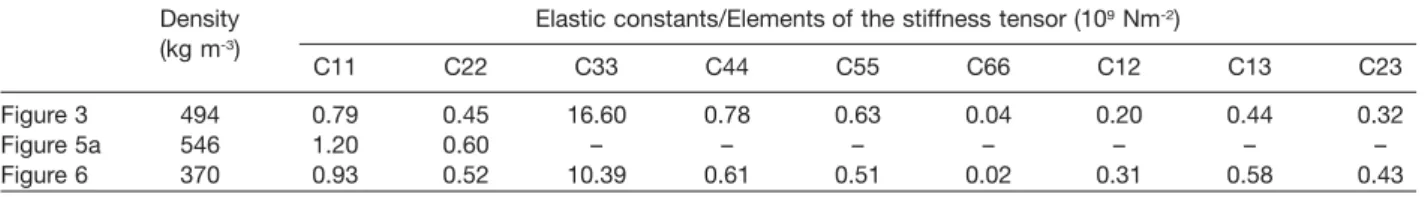
Table 1 Density and elastic constants (Cij) for the simulations according to the figures in which their results are depicted. Density Elastic constants/Elements of the stiffness tensor (109Nm-2)
(kg m-3)
C11 C22 C33 C44 C55 C66 C12 C13 C23
Figure 3 494 0.79 0.45 16.60 0.78 0.63 0.04 0.20 0.44 0.32
Figure 5a 546 1.20 0.60 – – – – – – –
Figure 6 370 0.93 0.52 10.39 0.61 0.51 0.02 0.31 0.58 0.43
Data in Figure 3 are according to Musgrave (1981). Data in Figure 6 are according to Hearmon (1948). rather a non-directional point source than a directional source.
The effects of such a point source on the waves being excited are described within the results for a 3D simulation model.
The digital signal was generated by LabVIEW and transmitted via the GPIB interface to the function generator (Stanford Research DS345), which converted the digital to an analog signal. The analog signal was amplified (Krohn-Hite 7500) and applied to the piezo stack. The bark of the investigated stem was not removed to keep conditions close to measurements on standing trees. The surface displacements of the bark are not equivalent to the displacements of the wood surface below the bark. Thus, the displacements were measured on top of the double thread screws by a heterodyne laser interferometer
(Polytec OFV3001). The tomographic measurements included the consecutive excitation of the trunk on each of the 24 posi-tions (Figure 3b), while in each case the displacements of the top of the remaining 23 double thread screws are measured. The displacements on the top of the screws are not exactly equal to the displacements of the wood surface below the bark, but the conditions are for all measurement points the same and thus the results are comparable. The resolution in the frequency range below 100 kHz was enhanced by combining the interferometer with the demodulator (MH PD4) (Dual et al. 1996). The measured signals were filtered with an analog filter (Krohn-Hite 3988) and digitized by an A/D converter (NI 5911) with 1 MHz sampling rate and an effective vertical resolution of 17.5 bit. The signals (300–1000 sweeps) were averaged in LabVIEW. During the sig-nal processing, the measured sigsig-nals were digitally filtered (a bandpass with pass frequencies between 10 kHz and 20 kHz of type Chebychew II and order 10).
Results and discussion
In their previous work (Schubert et al. 2006), the com-plexity of phenomena in a cylindrically anisotropic mate-rial was visualized by snapshots of P-, S-, and surface waves propagating in the rw-plane of a trunk. The simu-lations were carried out with a 2D model, which repre-sented the radial-tangential plane in a plane strain state. This 2D model is appropriate to calculate the travel times in the rw-plane. In contrast to the analysis of travel times, the analysis of waveforms and amplitudes of signals as well as energy flow requires a 3D model. The 3D model of the trunk, which was studied within this work, had an outer radius of Rs15 cm and a height of Ls70 cm. Since the simulations had to be comparable to the exper-iments, density and elastic constants of an example of spruce were chosen (Musgrave 1981, see Table 1). The trunk model was excited by applying a normal stress in radial direction at the outer surface. The excited surface area was 2 mm=5 mm and located in the middle of the trunk model length. The signal was a Hanning pulse with 3 periods of a sine and a center frequency of 50 kHz. The three snapshots in Figure 3 depict the absolute dis-placement of the waves propagating in the RZ-plane. The three snapshots are taken at ts0.0634 ms and they depict the same displacement amplitudes with different scaling. The white and black lines illustrate the analyti-cally calculated wave fronts of the P- and the two S-waves for a non-directional point source (Schubert 2007). It can be seen that the numerically simulated wave fronts are similar to the analytically derived wave fronts. The dimensions of the source in the numerical simulation are much smaller than the wave length of the P-waves in wood (8–35 cm for 15 kHz) and thus all types of waves are excited and propagate in all directions. The
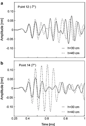
differ-Figure 4 Signals measured on locations 12 and 14 (Figure 5b) at different heights, while the trunk is excited at location 1 and the same height as the signals are measured.
ent scaling (factor 100) of the three snapshots at
ts0.0634 ms highlights the large geometrical spreading
of the energy, while the waves propagate in the trunk. That is to say, geometrical spreading is the significant parameter influencing the amplitudes of the measured signals besides material damping, which was neglected in the numerical simulation model. The coded information in the amplitude of measured signals concerning fungal decay is of second order of importance because of geo-metrical spreading of waves and material damping. Hence, such hidden information can only be reliably used if results of the investigated plane are compared with those of a reference rw-plane at the same tree. Such nor-malization of data with results of a reference plane has already been proposed by Socco et al. (2004).
To verify whether such reference planes on trunks are useful for comparing amplitudes, the signal forms were measured in the experiment on two different heights (ref-erence and investigated plane) of the spruce trunk. Fig-ure 4 depicts the signal shapes measFig-ured at locations 12 and 14 on different heights with 10 cm difference of the spruce trunk (Figure 5b). The amplitudes of the first cycles in Figure 4a are comparable in contrast to Figure 4b, where one signal is significantly larger. The signal shapes differ already after the first cycle.
After the experiments, the trunk was cut at the height of the measurement points to visually inspect the cross-sections. No knots or defects had been found to explain the different amplitudes. Figure 4 therefore indicates that the shapes of the signal as well as the amplitudes are very sensitive to the natural heterogeneity of the wood.
Nevertheless, the travel times varied at a maximum of 3% and proved to be less sensitive to the heterogeneity of the wood. Thus, in the section below the discussion is focused on the analysis of travel times or their equiv-alents, the average velocities.
The average velocities are calculated by dividing the distance between source and measurement point by the travel time between them. These travel times are deter-mined by an Akaike information criteria picker (Zhang et al. 2003). The relative position between source location and measurement point is described by the angle a, which is schematically depicted in Figure 1b, an example ofas458 for the source position 1 is given in Figure 5b. The average velocities depending on the anglea are in the following velocity curve v(a).
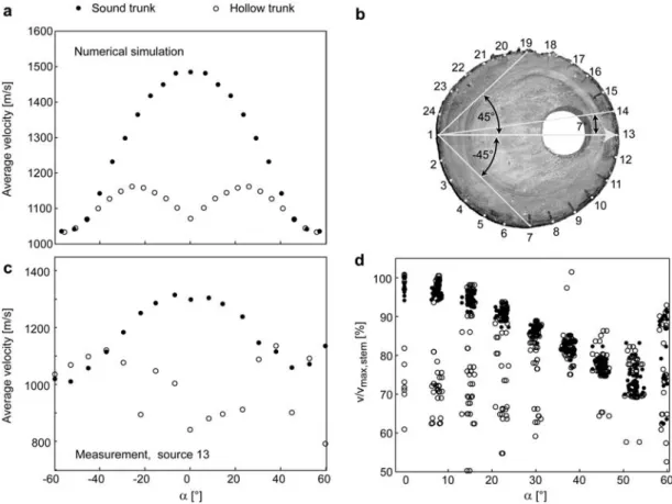
Figure 5a illustrates that the 2D simulation showed the velocity curve of sound trunks to be upside down v-shaped and of hollow trunks to be upside down w-shaped (Schubert et al. 2006). Table 1 summarizes the material parameters for the simulation. To verify the v-and w-shaped velocity curves, experiments on a spruce trunk before and after drilling a hole into the trunk were carried out (Figure 5b). Figure 5c depicts the velocity curves for the source point 13 before and after hole-drill-ing. The former (sound trunk) has indeed an upside down v-shape similar to the simulated curves. For the latter (hollow trunk), the velocity curve is upside down w-shaped but less regular than the simulation results. It is evident that for source locations, which do not lie on the symmetry axis of the hollow trunk, the w-shape is not symmetrical toas08.
Figure 5d depicts the velocity curves for all source points of the sound and the hollow trunk normalized by the maximum velocity of the sound stem versus the absolute value of a. The trunk with the hole is clearly distinguishable from the sound trunk in this velocity dia-gram. This result strengthens the assumption that AWT is a promising tool for detecting fungal decay in standing trees. However, experiments on other stems indicated that compression wood and branches may cause destructive interference of the waves. Due to destructive interference, the first-break onsets of the signals are erased and thus erroneous travel times are determined.
Travel times were less sensitive than amplitudes to the heterogeneity of wood. Nevertheless, the heterogeneity of wood is the limiting factor of AWT. For estimating the influence of the travel times, it is necessary to describe the heterogeneity in terms of the variation of material parameters (e.g., density and the elements of the stiff-ness tensor). The variation of C11(stiffness in radial
direc-tion) between reference and investigated plane influenced the velocity curve in a similar way as a decayed area (Schubert 2007).
The 2D numerical simulation model provides a power-ful tool to analyze the limit of detectability of fungal decay. The analyzing procedure was as follows: (1) the velocity curve of a reference model was computed, (2) the velocity curve of the C11model (19% decrease of C11
in the complete cross-section area, which results in a radial P-wave velocity of 90% of the one of the reference model) was computed, and (3) the velocity curves of
Figure 5 The experimental setup of the measurements and various velocity curves obtained by simulation and experiments. (a) 2D simulation of velocity curves of sound and hollow trunks. (b) Cross-section of the investigated spruce stem showing the excitation point 1 and various measurement locations. (c) Velocity curves of the sound and the hollow stem measured for the excitation on source point 13. (d) Velocity curves for all excitation points of the stem plotted versus the absolute value of a w8x.
models with various degrees and sizes of decay were computed. The material parameters of the reference model are summarized in Table 1.
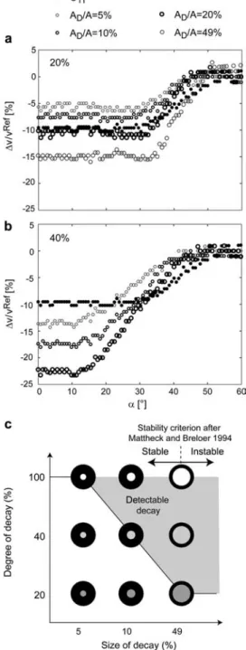
Figure 6a and b show the relative differences of the computed velocity curves of (2) and (3) with respect to the velocity curve of the reference model. The effect of the medium decayed models (20% decrease of the radial P-wave velocity) in Figure 6a is not distinguishable from the effect of C11on the velocity curve, unless the size of
the decay is very large (AD/As49%). This is in contrast
to the effect of the strongly decayed models (40% decrease of the radial P-wave velocity) in Figure 6b; these are all distinguishable.
Figure 6c summarizes the results of the analysis. According to Mattheck and Breloer (1994), the stability criterion for hollow trees is that the remaining sound wood thickness t has to be larger than 30% of the stem radius, which corresponds to AD/As49%. Thus, Figure
6c shows that AWT can detect a dangerous decay in sufficiently homogeneous trunks.
Conclusions
The heterogeneity of wood determines the detectability limit of AWT as well as certain limits of further develop-ment of the testing method.
Limit of detectability
Under the condition that no branches and no reaction wood lie in the investigated planes, the limit of detect-ability can be determined by the computation of velocity curves. It was shown for an example of spruce that it is possible to determine decayed areas that are large enough to endanger the stability of the trunk.
Restriction of further development
Since waveforms and amplitudes of the measured sig-nals were very sensitive to the variation of material para-meters within the difference of 10 cm in height, we conclude that wood tomography is restricted to travel time inversion. Further development towards waveform inversion is not promising.
Possible improvements
Wood tomography based on travel time inversion can be improved by normalizing the results of the investigated plane by the ones of a reference plane as recommended by Socco et al. (2004).
Tool for choice of reference planes
The velocity curve of the measured data provides a sim-ple and physically meaningful tool for supervising the
Figure 6 (a) Influence of decay and variation of C11 on the velocity curves. The decay was represented by areas with dif-ferent sizes (AD) and a reduction in the radial P-wave velocity of 20%. (b) Influence of decay and variation of C11on the velocity curves. The decay was represented by areas with different sizes (AD) and a reduction in the P-wave velocity of 40%. All simula-tions were carried out with the 2D simulation model with an outer radius Rs18 cm and the following discretization parameters:
Drs0.5 mm,Dts1.5=10-4ms. (c) Limit of detectability for cir-cular centered decay.
input data of wood tomography. This is important for the choice of appropriate reference planes.
Guiding questions for further research
Strong changes of material parameters in areas of a size comparable to the wavelength – e.g., branches or
reac-tion wood – may lead to erroneous travel time determi-nation and thus cause incorrect tomographic results. The analysis of the reliability of the AWT method should be guided by the following two questions: (1) how far does tension wood of hardwoods influence the wave propa-gation, and (2) how far can it be avoided that branches lie in reference or investigated planes.
References
Bulleit, W.M., Falk, R.H. (1985) Modeling stress wave passage times in wood utility poles. Wood Sci. Technol. 19:183–191. Dual, J., Ha¨geli, M., Pfaffinger, M.R., Vollmann, J. (1996) Exper-imental aspects of quantitative non-destructive evaluation using guided waves. Ultrasonics 34:291–295.
Gilbert, E.A., Smiley, E.T. (2004) Picus sonic tomography for the quantification of decay in white oak (Quercus alba) and hic-kory (Carya spp.). J. Arboricult. 30:277–281.
Hearmon, R.F.S. The Elasticity of Wood and Plywood. Technical Report. Department of Scientific and Industrial Research, London, 1948.
Madariaga, R. (1976) Dynamics of an expanding circular fault. Bull. Seismol. Soc. Am. 66:639–666.
Mattheck, C., Breloer, H. (1994) Field guide for visual tree assessment (VTA). Arboricult. J. 18:1–23.
Maurer, H., Schubert, S., Ba¨chle, F., Clauss, S., Gsell, D., Dual, J., Niemz, P. (2006) A simple anisotropy correction procedure for acoustic wood tomography. Holzforschung 60:567–573. May, F., Dual, J. (2006) Focusing of pulses in axially symmetric
elastic tubes with fluid filling and piezo actuator by a finite difference simulation and a method of time reversal. Wave Motion 43:311–322.
Musgrave, M.J.P. (1981) On an elastodynamic classification of orthorhombic media. Proc. R. Soc. Lond. 374:401–429. Nicolotti, G., Socco, L.V., Martinis, R., Godio, A., Sambuelli, L.
(2003) Application and comparison of three tomographic techniques for detection of decay in trees. J. Arboricult. 28: 3–19.
Payton, R.G. (2003) Wave fronts in wood. Quat. J. Mech. App. Math. 56:527–546.
Rabe, C., Ferner, D., Fink, S., Schwarze, F.W.M.R. (2004) Detec-tion of decay in trees with stress waves and interpretaDetec-tion of acoustic tomograms. Arboricult. J. 28:3–19.
Schubert, S., Gsell, D., Dual, J., Motavalli, M., Niemz, P. (2006) Non-destructive testing of trunks: studying elastic wave propagation by numerical simulation. Wood Res. 51:11–24. Schubert, S. Acousto-ultrasound assessment of inner
wood-decay in standing trees: possibilities and limitations. Diss ETH Nr. 17126, Zu¨rich, 2007. http://e-collection.ethbib. ethz.ch/cgi-bin/show.pl?typesdiss&nrs17126.
Socco, L.V., Sambuelli, L., Martinis, R., Comino, E., Nicolotti, G. (2004) Feasibility of ultrasonic tomography for non-destruc-tive testing of decay on living trees. Res. Nondestruct. Eval. 15:31–54.
Yee, K.S. (1966) Numerical solution of initial boundary value pro-blems involving Maxwell’s equations in isotropic media. IEEE Trans. Ant. Prop. 14:302–307.
Zhang, H., Thurber, C., Rowe, C. (2003) Automatic P-wave arri-val detection and picking with multiscale wavelet analysis for single-component recordings. Bull. Seismol. Soc. Am. 93: 1904–1912.