HAL Id: hal-01274035
https://hal.inria.fr/hal-01274035
Submitted on 15 Feb 2016
HAL is a multi-disciplinary open access archive for the deposit and dissemination of sci-entific research documents, whether they are pub-lished or not. The documents may come from teaching and research institutions in France or abroad, or from public or private research centers.
L’archive ouverte pluridisciplinaire HAL, est destinée au dépôt et à la diffusion de documents scientifiques de niveau recherche, publiés ou non, émanant des établissements d’enseignement et de recherche français ou étrangers, des laboratoires publics ou privés.
Systems
Florent Jacquemard, Clément Poncelet
To cite this version:
Florent Jacquemard, Clément Poncelet. An Automatic Test Framework for Interactive Music Systems. Journal of New Music Research, Taylor & Francis (Routledge), 2016, 45 (2), pp.18. �hal-01274035�
Florent Jacquemard and Clement Poncelet
Sorbonne Universit´es, Inria, UPMC Univ Paris 06, IRCAM – CNRS UMR SMTS, Paris, France
Abstract
Score-Based Interactive Music Systems are involved in live performances with human musicians, reacting in realtime to audio sig-nals and asynchronous incoming events ac-cording to a pre-specified timed scenario called mixed score. Building such a system is a difficult challenge implying strong require-ments of reliability and robustness to unfore-seen errors in input.
We present the application to an automatic accompaniment system of formal methods for conformance testing of critical embedded sys-tems. Our approach is fully automatic and based on formal models constructed directly from mixed scores, specifying the behavior expected from the system when playing with musicians. It has been applied to real mixed scores and the results obtained have permit-ted to identify bugs in the tespermit-ted system.
Keywords: model based conformance
testing, realtime systems, score based inter-active music systems, generation of artificial music performances.
∗
This work has been partly supported by a DGA-MRIS scholarship and the project Inedit (ANR-12-CORD-009).
Introduction
Interactive music systems (IMS) [23] play in live music performances with human musi-cians. They work by coupling functionalities of artificial listening, for score following and tempo detection, and of reactive systems, for coordinating their outputs with musician in-puts. In the case of score-based IMS, all these activities are performed in realtime, following a pre-specified timed scenario called a mixed score, written in a Domain Specific Language (DSL). It defines the parts of human musi-cians (input) together with electronic parts (output) and their synchronization.
During an instrumental performance, when a musician does a mistake, the piece must and will continue. However, IMS practitioners know that a misbehavior of an IMS can jeop-ardize a mixed instrumental-electronic per-formance. In order to built reliable IMS and meet listeners’ expectations, it is important to be able to explore, statically, the IMS re-actions to as many as possible musician’s in-terpretations, and check that these reactions conform to the behavior specified in the given mixed score. This difficult task is compli-cated by high unpredictability of musicians’ inputs and hard temporal constraints (due in particular to the strong requirements of audio computing platforms).
rehearsing with musicians. However time is precious during a rehearsal, whose purpose is usually more to solve musical problems than to fix bugs. It is also possible for develop-ers to listen to recordings of an IMS play-ing with some musicians, checkplay-ing a poste-riori that the result sounds satisfiable. The problem with this approach is that, on the one hand, the test input is not complete (it just represents one or a few particular perfor-mances) and has to be played entirely, so such a testing procedure is tedious and time con-suming. On the other hand the verification of the outcome is not rigorous.
This paper presents a study of the applica-tion of Model-Based Testing (MBT) meth-ods to the score based IMS Antescofo, de-veloped at Ircam and used regularly in con-certs. This system shares several character-istics with the critical systems traditionally targeted by MBT, such as reactivity and re-altime semantics.
The main originality of our contribution is the automatic construction of a formal model M of the system’s IO behavior from a given mixed score, using a front-end compiler into an ad hoc intermediate representation (IR). In this approach, the score is seen as a spec-ification of the expected system’s behavior. This is in contrast with usual MBT case stud-ies where the model has to be built manually by an expert. On the base of the constructed model, we address the following issues: (i) exhaustive generation of test data for in-put, including timing values (artificial per-formances), following covering criteria, and applying model-checking techniques to M, (ii) computation of the corresponding ex-pected output data, according to the input and the model, hence the mixed score, (iii) black-box execution of the generated test data using virtual clocks in order to play in a fast-forward mode. The outcome of the system is then compared formally to the ex-pected outputs to check a Relativized Timed Input/Output Conformance relation (rtioco) between traces and a user readable verdict is produced.
Although the paper present an application to a specific IMS, our framework is based on a generic model (the IR), and could therefore be applied to other score-based IMS using, like Antescofo, a reactive DSL (relating dis-crete output to disdis-crete input, with time val-ues). Providing a compiler from a DSL into our IR (such as our adhoc front-end compiler from Antescofo DSL into IR), one could reuse our framework for the above steps (i) and (ii) without modifications. Note also that the steps of our workflow are independent, and linked using a generic timed trace format.
Structure of the paper. In the first part of the paper (Section 1), we present our model-based testing approach from the point of view of the user, considered as an exter-nal observer. We first present briefly our tar-get system Antescofo and its DSL for writing mixed scores (1.1, 1.2). Then we define the format of the test data (traces), in input and output (1.4), and describe our testing work-flow (1.3, 1.5, 1.6).
The second part (Section 2) details the in-ternals of our test procedure, i.e. the mod-els of the system’s behavior (2.1) and how they are used to generate test data. We use the symbolic model checker Uppaal [14] and its extension CoVer [6], both based on the standard model of Timed Automata [3], for the production of test input and output data, with some covering criteria (2.2). We also propose alternative techniques for pro-ducing test input data: fuzzing of an ideal trace using performance models of the liter-ature (2.3), and the generation of input data from audio recordings (2.4).
Finally, we present (Section 3) some rele-vant experimental case studies, the first one based on a benchmark of several hundreds of small mixed scores, and the other based on an extract of the real piece of mixed music Einspielung by Emmanuel Nunes.
Related Work. Some tools exists for au-tomating the test of IMS, like for instance the max-test package [18] for testing MAX
musicians mixed score audio software Listening Machine Reactive Engine audio or
MIDI stream tempo
pos.
messages
Figure 1: Architecture of Antescofo
patches through assertions. These systems conveniently provide sophisticated tools for automating execution of test data and re-porting. But they generally do not offer pro-cedures for generating test data, hence the user must compute some input test data and the expected corresponding output by other means. Our approach ([19, 20]) in contrast focus on the generation of test data, based on formal models, and in this respect the two approaches can been seen as complementary. Other work has addressed the formal verifi-cation of multimedia systems based on Timed Automata models, such as for instance the verification of a lip-synchronisation protocol (synchronization of audio and video streams) in [7]. Timed Automata Networks, Uppaal, as well as timed Petri nets, are used in i-Score [5], a framework for composition, verifi-cation and real-time performance of Multime-dia Interactive Scenarios. To our knowledge, no other work has applied such formal models to the test of Interactive Music Systems.
1
IMS Test Framework
We introduce in this section our case study, the score follower Antescofo (1.1), its domain specific language (DSL) for writing mixed scores (1.2), our Model-Based Testing (MBT) workflow (1.3), whose main steps are the gen-eration of test cases, the execution on the sys-tem under test (1.5) and test verdict (1.6). Test cases are timed traces, which is the for-mat for data exchange in our test frame-work (1.4). Their generation from models is presented in Section 2.
1.1 The IMS Antescofo
Figure 1 describes roughly the architecture of Antescofo, which is made of two main mod-ules. A listening machine (LM) decodes an audio or midi stream incoming from a musi-cian and infers in realtime: (i) the musimusi-cian’s position in the given mixed score, (ii) the mu-sician’s instantaneous pace (tempo, in beats per minute) [8]. These values are sent to the second module: a reactive engine (RE) which schedules the electronic actions to be played, as specified in the mixed score. The actions are messages (i.e. instructions) emitted on time to an audio environment: a realtime au-dio software such as MAX/MSP [21] or Pure Data [22], in which Antescofo is embedded as a patch.
Therefore, from a behavioral point of view, the RE can be seen as a reactive system re-ceiving and sending discrete events: some in-put events sent by the LM to the RE and output events sent by the RE to the environ-ment. We propose a uniform format for these events in Section 1.4.
1.2 Domain Specific Language
The mixed scores of Antescofo are written in a textual language allowing the description of the electronic accompaniment in reaction to the detected instrumental events. A simpli-fied extract of the score of Einspielung I1 by Emmanuel Nunes is presented in Figure 2. This piece for violin and electronics will be used as a running example in this paper.
Example 1. Figure 2 displays the first bar of Einspielung’s mixed score in Antescofo DSL. The violin part is represented in com-mon western music notation in Figure 3. The keywords note and chord in Figure 2 are used to represent the input events expected from the violin (chords represent double stops). They are followed by a note pitch (or list of pitches), a duration (always 17 in the example) and a label (e1, . . . , e7). The
electronic part is specified with actions and sequences of actions called groups. Each ac-tion is expressed with a delay (time to wait before throwing action) followed by a message (abstract symbols a0, . . . , a7 in the example).
A group is expressed with a delay, a label (s2 in the example) followed by a sequence of
actions or nested groups.
The interleaving of notes/chords and se-quences of actions and groups specifies the coordination between input events and out-put actions: a sequence of actions (a0, s2 . . . )
is triggered by the previous note (e1 in the
example). A zero delay between a trigger-ing note and the first triggered action means simultaneity: for instance both a0 and the
group s2 are started (in this order) as soon as
e1 is detected. Note that the total duration
of the group s2 is bigger than the duration
of the triggering event e1 (1 vs 17). It means
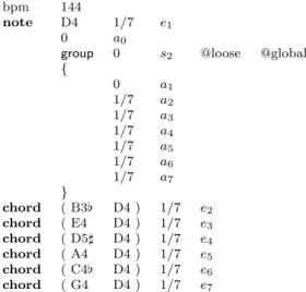
bpm 144
note D4 1/7 e1
0 a0
group 0 s2 @loose @global
{ 0 a1 1/7 a2 1/7 a3 1/7 a4 1/7 a5 1/7 a6 1/7 a7 } chord ( B3[ D4 ) 1/7 e2 chord ( E4 D4 ) 1/7 e3 chord ( D5] D4 ) 1/7 e4 chord ( A4 D4 ) 1/7 e5 chord ( C4[ D4 ) 1/7 e6 chord ( G4 D4 ) 1/7 e7
Figure 2: The first bar of Einspielung’s mixed score in Antescofo DSL (simplified).
Figure 3: The first bar of Einspielung’s violin part in common western notation.
BPM 144 evt(e1, 1/7, s1); evt(e2, 1/7, [ ]); evt(e3, 1/7, [ ]); evt(e4, 1/7, [ ]); evt(e5, 1/7, [ ]); evt(e6, 1/7, [ ]); evt(e7, 1/7, [ ]) where s1 = act(0, [a0], [ ]);
act(0, s2, [loose; global])
s2 = act(0, [a1], [ ]); act(1/7, [a2], [ ]); act(1/7, [a3], [ ]); act(1/7, [a4], [ ]); act(1/7, [a5], [ ]); act(1/7, [a6], [ ]); act(1/7, [a7], [ ])
Figure 4: Abstract syntax for the mixed score of Figure 2.
that the execution of this group will continue in concurrence with the detection of the next
events e2, . . . , e7. ♦
The DSL of Antescofo offers an important set of features described in [12]. Composers can use different strategies of synchroniza-tion with the musicians’ inputs for accom-paniment, and different errors management strategies etc. We present here a simplified abstract syntax corresponding to a fragment of this language, in order to illustrate our test framework.
Let O be a set of output messages (also called action symbols and denoted a) which can be emitted by the system and let I be a set, disjoint from O, of event symbols (de-noted e) to be detected by the LM (i.e. positions in score). An action is a term act(d, s, al ) where d is the delay before start-ing the action, s is either an atom in O or a finite sequence of actions, and al is a list of attributes. A mixed score is a finite sequence of input events of the form evt(e, d, s) where
e ∈ I, d is a duration and s is the top-level group triggered by e. Sequences are denoted with square brackets [ , ] and the empty se-quence is denoted [ ]. Figure 4 depicts the running example in the abstract syntax.
The high-level attributes attached to an action act(d, s, al ) are indications regarding musical expressiveness [9, 12]. We consider here four attributes for illustration purpose, two attributes are used to express the syn-chronization of the group s to the musician’s part: loose (synchronization on tempo) and tight (synchronization on events) and two at-tributes describe strategies for handling er-rors in input: local (skip actions) and global (play actions immediately at the detection of an error).
We define an error as an event of the score missing during the performance, either be-cause the musician played a wrong note, did not play it at all or because it was not de-tected by the LM.
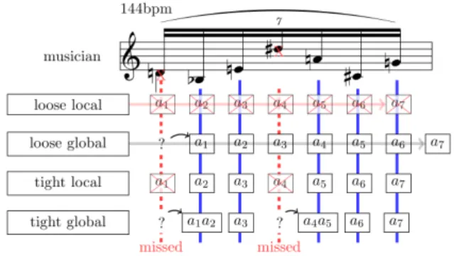
Example 2. Figure 11 illustrates An-tescofo’s behavior for various combinations of attributes for the group s2 of our running
example. Note that in Figures 2 and 4, the attributes loose and global are selected. ♦ Allowing the user to express error handling strategies and different degrees of smooth-ness for the system reactions are interesting features in a context of music composition but can complicate the understanding of the
Figure 5: Reactions for various combinations of attributes for s2, when the
events e1 and e4 are missed.
mixed scores and their validation.
1.3 Test Workflow
A mixed-score is seen in our case as a specifi-cation describing precisely the timed behav-ior expected from the system during a per-formance. It expresses the durations of input events (from the musician) corresponding to an ideal performance. In practice, real per-formances are not (and should not be) ideal: the tempo of the musician will be fluctuating, some notes’ durations can be shifted and ac-cidents can also occur (missing notes). The set of real performances is then infinite and no two performances will be the same. The purpose of a good test procedure is to assess the response of the system to a representative set of performances, as covering as possible.
Several formal methods have been devel-oped for automatic conformance testing of critical embedded software, see e.g. [17]. Here we follow a Model-Based Testing (MBT) ap-proach, where a formal model is used to con-struct representative performances and ex-pected system’s answers. Tests are executed with a real implementation under test (IUT), seen as a black-box (the source code of the IUT is not known and only the inputs and outputs are observed).
More precisely, in conformance MBT methods, a formal model M of the system is needed. In general it is written manually by an expert. In our case however, it is ob-tained automatically by compilation of the mixed score, which is assumed to contain suf-ficiently information about the behavior ex-pected from the system. Indeed, by essence,
mixed score specification S
perf. info
E or data input traces
expected output traces simulation
real output traces comparison verdict
compilation
generation execution
a mixed score describes precisely the relation between the outputs of the system and musi-cian’s events, with timing information. Such a scenario is very convenient in a context of assistance to composers of musical produc-tions, who are usually subject to strict calen-dar constraints.
The model (see Section 2.1) is composed of two parts: S the specification, describing the behavior expected for the IUT, and E the environment, defining the inputs possible during the tests. The Model is used (Fig-ure 6 and Section 2.2) to generate automati-cally some relevant test data: the input trace tin, sent to the IUT, which must conform
to E , and the theoretically expected output trace tout, computed from tin by simulation
using S. On the other hand, an execution of the IUT on tinpermits to monitor real output
trace t0out, which is then compared to tout in
order to produce a test verdict.
1.4 Input and Output Test Data
For realtime systems such as communication protocols, transportation control etc, as for IMS, time is a semantic issue, not just a measure of efficiency. Therefore, the test traces tin and tout must be timestamped.
We consider two time units here: physi-cal time, in seconds, and musiphysi-cal time, ex-pressed in number of beats relatively to a tempo. Let us assume a tempo curve τ as-sociating an instant tempo value, in beats per minute (bpm), to each date t (in phys-ical time). The conversion of a duration d from musical time into physical time is ob-tained by integration in [0, d] of the inverse of τ . Here, we shall always consider tempo curves which stay constant between the oc-currences of two events. This corresponds to the assumption (used in Antescofo LM) that we infer tempo variations only at the arrival of events, and not in-between.
A timed trace is a sequence of triples hai, ti, pii made of a symbol ai ∈ I ∪ O,
a timestamp ti ∈ R+ (onset ), expressed in
musical time, and a tempo value pi in bpm,
such that for all i, ti ≤ ti+1 and if ti = ti+1
then pi+1 = pi. The tempo curve τ
associ-ated to such a trace is defined by τ (t) = pi
iff ti ≤ t < ti+1. A trace containing
sym-bols exclusively in I (resp. O) is called an input trace (resp. an output trace). We de-note below Tin (resp. Tout) the set of input
(respectively output) traces with timestamps in musical time (tbeat). The ideal trace for a
mixed score S is the input trace of Tin
con-sisting in the projection of all input events in S with their date (accumulated duration) and the tempo given in S.
Example 3. The ideal trace for the score in Figure 2 is:
he1, 0, 144i·he2,17, 144i· . . . ·he6,57, 144i·he7,67, 144i.
♦ Let us consider the two parts of model de-fined above E as a set of possible input traces and S as a simulation function from input traces to output traces. A test case is a pair htin, touti ∈ Tin × Tout where tin ∈ E is an
input trace (an artificial performance) and tout = S(tin) is the corresponding expected
system’s reaction. The automatic and cov-ering generation of input traces tin and
ex-pected output traces tout from scores is the
topic of Section 2.
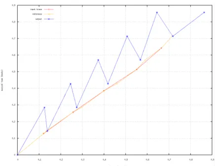
Example 4. Let us consider the three fol-lowing input traces for the piece in Figure 2.
t1in = he1, 0, 114i · he2,17, 117i · he3,27, 120i·
he4,37, 117i · he5,47, 114i · he6,57, 111i·
he7,67, 114i.
t2
in = he1, 0, 114i · he3,143, 120i · he4,146, 117i·
he6,149, 111i · he7,1214, 114i.
t3
in = he1, 0, 114i · he2,709, 117i · he3,1870, 120i·
he4,2770, 117i · he5,3670, 114i·
he6,4570, 111i · he7,5470, 114i.
In trace t1in the durations are those of the mixed score but the tempo diverges from the ideal tempo (unlike Example 3). In t2
in, the
onsets are shifted (to play the events a bit earlier or later) and events e2, e5 are missed.
In the last trace t3
inall events are played 10%
Figure 7: Input traces t1in, t2inand t3in, physical values according relative ones.
1.5 Test Execution
Having defined a format for timed traces, the next question is: How can we observe the re-action of the system to a given input?
The execution of an input trace tinis
some-how a monitored simulation of a performance. It consists in sending the events in tin to the
IUT, at the specified dates, and collect a real output trace t0out by monitoring and time-stamping all output emitted by the system during the execution.
The problem can be complex due to the data flow in Antescofo, its modular nature (Figure 1) and the variety of time units that can be used in timed traces. We present below several scenarios for testing different parts of the system corresponding to differ-ent boundaries for the black box tested.
1.5.1 Testing the Reactive Engine
This scenario is performed with a standalone version of Antescofo equipped with an inter-nal test adapter module. The adapter itera-tively reads elements hai, ti, pii of tin in a file.
The duration dmui = ti+1− ti of the event ei
(in musical time) is converted into physical
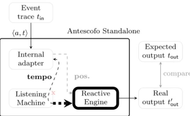
Antescofo Standalone Event trace tin Internal adapter Listening Machine Reactive Engine ha, t, pi tempo x pos. x Real output t0out Expected output tout compare
Figure 8: Testing scenario of Section 1.5.1.
time by: dphi = d mu i .60 pi (1)
The adapter then waits for dphi seconds before sending ei+1 and pi+1 to the RE.
More precisely, it does not physically wait, but instead notifies a virtual clock in the RE that the time has flown by dphi seconds. This way the test does not need to be executed in realtime but can be done in a fast-forward mode. This is very important for batch exe-cution of huge sets of test cases.
The messages sent by the RE are logged in t0out, with timestamps in physical time (i.e. with a tempo of 60bpm). In this scenario, the
IUT is the RE (the LM is idle).
1.5.2 RE with Tempo Detection
In this second scenario, tempo values pi read
in tin are ignored by the adapter, which
in-stead uses the tempo values inferred by the LM (the adapter is calling an appropriate method of the LM) in order to compute the events’ durations dphi . The rest of the sce-nario is similar to Section 1.5.1. The values of tempo inferred by Antescofo’s LM are stored by the adapter and used later to convert the timestamps in the expected output trace tout
from musical to physical time, in order to be able to compare it with the real output trace t0out. In this case, the IUT consists in the RE plus the part of the LM in charge of tempo inference. The LM infers the tempo based on the shift between durations in tin
and in the mixed score [8]. It might result in a tempo increasing exponentially when dura-tions in tin are too short.
Example 5. Let us see how the detected tempo can increase by executing our trace t3in via this scenario. The duration of e1 is
computed with the timestamp of e2 found in
t3in: dmu1 = 709 − 0. Then we obtain a phys-ical value of dphy1 = 0.05357 seconds with a tempo of 144 (score value by default). The detection of e2 is earlier than expected (since
the relative time is shorter than 10%), An-tescofo’s LM modifies its current tempo to 146bpm. The computation of the same
rela-Antescofo Standalone Event trace tin Internal adapter Listening Machine Reactive Engine ha, ti tempo pos. x Real output t0out Expected output tout compare
Figure 9: Testing scenario of Section 1.5.2.
tive duration for the next event is done with a faster tempo and gives dphy2 = 0.05283 sec, the event is earlier so the next tempo is faster than 146bpm and so on. In this very short ex-ample (and with small shifted durations), we reach at the end a tempo of 150.3bpm, that is 6.3bpm more than the score tempo in 0.4
seconds of a performance. ♦
1.5.3 Testing the Whole System
This scenario is the most general. It is exe-cuted with a version of Antescofo embedded in MAX (as a MAX patch), using an adapter which is another MAX patch. The adapter iteratively reads triples hai, ti, pii in a file
containing tin, and converts them into MIDI
events, with durations dphi casted into phys-ical time using (1). The events are played by the MAX patch midisynth˜ and the audio stream generated is sent to the LM. The out-put of the RE is then traced in t0out as before. Note that here, the RE uses the tempo values detected by the LM, which may dif-fer from the tempo values in tin. The
de-tected tempo values are saved by the adapter (in MAX the detected tempo is available as an outlet of the antescofo˜ patch). They are used later to convert the dates in tout
from musical into physical time, like in Sec-tion 1.5.2. In this realistic scenario, the IUT is therefore the whole Antescofo system.
In an alternative scenario, the adapter uses the tempo values pi in tin for computing the
events’ durations dphi , like in Section 1.5.1.
Event trace tin External adapter (MAX patch) Listening Machine Reactive Engine audio stream tempo pos. Real output t0 out Expected output tout compare
Figure 10: Testing scenarios of Section 1.5.3.
Note that in both scenarios of this section, the tests are executed in real-time and not in a fast-forward mode like in Sections 1.5.1 and 1.5.2. However an audio file of the se-quence of MIDI sounds can be recorded and sent later to the standalone in fast-forward mode.
1.6 Comparison and Verdict
How can we check that the real output trace t0out is correct? When the expected output trace tout is not precisely defined, we are left
to listen to the execution of the IMS on tin,
in extenso, for instance using the framework presented in Section 1.5.3, and decide subjec-tively whether we are satisfied with it. This manual solution is not precise and also te-dious when one needs to consider many dif-ferent tin for covering purposes.
In our approach, we compute tout from tin,
as described in Section 2, and the verdicts are produced offline by a tool comparing the expected output trace tout to the monitored
output trace t0out (after conversion of times-tamps into physical time as described above). One difficulty for the comparison of traces is that some messages might be missing in t0out or the order of close messages might be inverted. We do not use a simple componen-twise comparison between tout and t0out, but
instead compares the respective dates of each symbol in these two output traces. For the comparison we use a fixed tolerance bound δ, for dealing with latency. In the reported ex-periments, we have used δ = 0.1ms.
Example 6. A running example is done to present an error case seen during an Antescofo’s test. Let us consider the input trace t4in derived from t3in with the first event missing and the tempo divided by two. The beginning of the corresponding expected and real output traces (respec-tively t4out and t04out) are reported below and the verdict is depicted in Figure 12.
t4
in = he2, 0, 62i · he3,709, 64i · he4,1870, 60i·
he5,2770, 58i · he6,3670, 56i · he7,4570, 58i.
t4out = he2, 0, 62i · ha0, 0, 62i · ha1, 0, 62i·
ha2, 0, 62i · he3, 0.12856, 64i·
ha3, 0.14285, 64i . . .
t04out = ha0, 0, 60i · ha1, 0, 60i · he2, 0, 60i·
he3, 0.12442, 60i · ha2, 0.13781, 60i·
he4, 0.24495, 60i · ha3, 0.27353, 60i . . .
In the expected trace t4out, the tempo values are copied from the input trace t4in. Since the event e1 is missed in t4in, and according to
the group attributes in Figure 3, a0, a1 and
a2 are sent immediately when e1 is detected
as missing i.e. at the detection of e2. The
delays in the real trace t04out are in physical time (60 bpm). Note that in this trace, a0 and a1 are before e2, contradicting the
order in t4out. However this does not alter the conformance because all these events are synchronous (time-stamp 0s). In contrast, the action a2 is at 0 in t4out and not in t04out,
this is reported as an error in the verdict (Figure 12): the real trace t04outis not conform to t4out, indicating a bug in Antescofo. ♦
2
Models
and
Automatic
Test Cases Generation
It remains to see how to generate the test cases htin, touti. We present below several
ap-proaches based on models built from a given mixed score for creating a relevant and cover-ing set of input traces tinand computing the
corresponding expected output traces tout.
2.1 Models of Computation
The principle of MBT approaches is to rely on a formal model M specifying the good be-havior of the IUT. This model acts as an ora-cle computing the good outputs from a given input trace. As observed in Section 1.3, a mixed score describes formally the outputs of the system following musician’s events (with timing information). Therefore, it is used in order to create automatically the model M at the heart of our approach. More precisely, M is constructed from an Abstract Syntax Tree (Figure 4), itself obtained by parsing a program in Antescofo DSL (Figure 2).
Figure 11: Traces t4in, t4out and t04out, physical values according relative ones.
2.1.1 Intermediate Representation
We use an Intermediate Representation (IR) for defining the formal models M of our MBT framework. An IR program is a finite set (called network ) of Finite State Machines (FSM) with durations, communicating syn-chronously with some symbols taken from a finite alphabet. Formally, an FSM is a tu-ple S = hΣin, Σout, L, `0, T i where Σin and
Σout are finite sets of respectively input and
output symbols (they may have a non-empty intersection), L is a finite set of locations, `0 ∈ L is the initial location, T ⊆ L × L
is a set of transitions labeled with one of: σ! with σ ∈ Σout – emission of a symbol,
τ ? with τ ∈ Σin – reception of a symbol,
[d, d0] where d, d0 ∈ R+ are expressed in the
same time unit (musical or physical) – wait for a delay between d and d0. A branch is made of a location ` ∈ L and the set of transitions outgoing from `. A FSM is called deterministic iff it contains no branch with more than one emit transition and for every wait transition labeled [d, d0], it holds that d = d0 (in this case, we simply write d instead of [d, d]).
The execution of an IR program is based on a notion of logical time. Initially, the logical time is set to 0 and every FSM of the IR program is in its initial location `0.
Activating in a FSM a transition tr labeled with [d, d0] makes the logical time advance by a duration between d and d0. More precisely, if the current logical instant is t ∈ R+, ` is
the source location of tr and the logical time already spent in ` is γ, then the logical time can be advanced to the new current logical instant t + γ + δ if γ + δ ∈ [d, d0].
Activating a transition labeled with σ! does not change the current logical instant (such a transition is considered as instantaneous). The symbol σ is recorded in a store and will be readable during the current logical instant, but not after: the activation of a transition labeled with [d, d0] flushes the store.
A transition labeled with τ ? can be acti-vated if τ is present in the store. Such a transition does not change the current logi-cal instant and neither changes the store.
Some examples of IR and their executions are given in Section 2.1.2.
_____________________________________________________________________________
|- Antescofo Trace | Expected Trace -|
|- label now [rnow] |label comp. timestamp [ref beat] -|
|---| | a0 0 [0.142857] | a0 0 [ 0] | | a1 0 [0.142857] | a1 0 [ 0] | | e2 0 [0.142857] | e2 0 [ 0] |* 62BPM + 0.124423 (0.142857 * 62) > 0.124413 (0.12856 * 62) | e3 0.124423 [0.285714] | e3 0.124413 [0.12856] |* 64BPM + 0.0133942 (0.0142871 * 64) > -0.124413 (-0.12856 * 64) x a2 0.137817 [0.300001] x a2 0 [ 0] delta:0.137817 + 0.10714 (0.12857 * 64) > 0.107128 (0.11427 * 64) | e4 0.244957 [0.428571] | e4 0.244938 [0.25712] |* 60BPM + 0.0285743 (0.0285743 * 60) > -0.107128 (-0.11427 * 60) x a3 0.273531 [0.457146] x a3 0.13781 [0.14285] delta:0.135721 [...] + 0.0857229 (0.0857229 * 60) > -0.0591 (-0.05713 * 60)
|---END TIMESTAMP OF REF TRACE---|
x a7 0.86301 [1.08572] x a7 0.718148 [0.71425] delta:0.144863
|---| Error :: Test KO
Figure 12: Part of a verdict for the comparison of t4out with t04out. The mark ’+’ indicates a new logical instant (see Section 2.1). The differences between the ideal trace and the input
trace are shown with ’<’, ’>’ and ’==’. The mark ’x’ indicates an error.
2.1.2 Compiling Mixed Score into IR
For the sake of conciseness, we shall not de-scribe in details the construction of models from mixed scores. We will instead explain its principles on some examples. The formal model M is made of two parts: a FSM E defining the possible behaviors of the envi-ronment (subset of Tin, see Section 1.4), and
a network S specifying the behavior expected from the system (function from Tininto Tout).
The sets of O and I are those of Section 1.2. We assume in addition a set Sigs of symbols of internal signals, disjoint from O and I.
Environment. The environment E is
a non-deterministic FSM of the form
hO, I, Le, `0, Tei.
Example 7. Figure 13 presents an exam-ple of environment model E for the three first events of the piece in Figure 4. It models a musician which, in `0, will possibly play the
first note e1, or miss it (upper edge labeled
with e2! targeted to `3) or miss e1 and e2
(edge labeled with e3! targeted to `5). When
`0 e1! `1 `2 `3 `4 `5 [0.1, 0.2] e2! [0.1, 0.16]? e3! e2! e3!
Figure 13: FSM for an environment E modeling the 3 first events of the piece.
e1 is not missed, this note must have a
dura-tion between 0.1 and 0.2 t.u. These bounds define a tolerance for negative or positive shifts to the duration of 17 in the score. ♦ For a given score, there are several options regarding missed notes and duration bounds (which will be source of non-determinism in E ). They are given by users in the com-mand for compiling.
Error Proxy. In Section 1.2, we have de-fined the errors as missed events. An FSM of the form hI, Sigs, Lp, `0, Tpi, called a proxy, is
in charge of signaling such errors, using one internal signal ei ∈ Sigs for each input event
ei∈ I. These signals are then handled by the
`0 `1 `2 `3 `1 `2 `3 e1? e2? e3? e2? e1! e3? e1! e2 ! e3?
Figure 14: Proxy FSM P with 3 events.
Example 8. In the proxy P displayed in Figure 14, in location `0, at the detection of
e2 (instead of e1), the signal e1 is sent. And
at the detection of e3, the signals e1 and e2
are sent. ♦
The use of this proxy FSM will simplify the complex task of specifying error handling in the other FSMs of the model S. In par-ticular, such a modular approach permits to change the definition of errors without having to change the rest of the specification S.
FSM for Groups. Finally, we associate several FSM to the mixed score, one for each group. The FSM for a group s has the form Gs= hI ∪ Sigs, O ∪ Sigs, Ls, `0, Tsi. It means
that Gs will receive input events and
inter-nal siginter-nals and send, in reaction, output mes-sages and other internal signals.
Example 9. Figure 15 presents the FSM Gs1 associated to the top-level group s1
trig-gered by the event e1 in the mixed score of
our running example Figure 4. The FSM Gs1
is started by the reception of one of the input symbol e1 ∈ I or the internal signal e1 ∈ Sigs.
In the first case, the FSM continues in a nor-mal mode (location `1). Otherwise it
contin-ues in an error mode (location `1). The FSM
Gs2 corresponding to the nested group s2(see
Example 10) is started by the emission of one of the internal signals s2 or s2. ♦
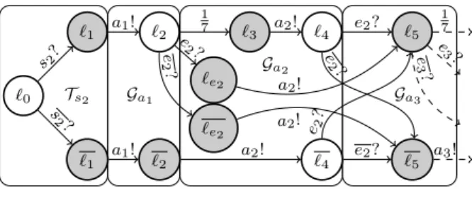
Example 10. Figures 16 and 17 show the FSM Gs2 obtained from the group s2 in
Figure 4, for two different synchronization strategies (resp. loose and tight). Those mod-els are constructed by iteratively traversing the sequence of actions in s2. The parts built
`0 `1 `1 `2 `2 `3 `3 e1? e1 ? a0! a0! s2! s2!
Figure 15: The FSM Gs1 for the group s1.
`0 `1 `1 `2 `2 `3 `3 `4 `4 `13 `13 `14 `14 s2? s 2? a1! a1! 1 7 e2? e2? a2! a2! 1 7 e7? e7? a7! a7! Ts2 Ga1 Ga2 Ga7 F
Figure 16: The FSM Gs2 for the group s2
with attributes loose, global.
at each step are framed and annotated as Tg (start of the group, triggered by one of the internal signals s2 and s2), Ga (for
han-dling one atomic action a), or F (end of the group). The dashed transitions indicate a missing part of the representation (too long for being presented entirely).
In Figure 16 (attributes loose, global), the top part of the IR (locations `1, ..., `14)
de-scribes a mode with a normal behavior (ab-sence of errors). It consists in sending suc-cessively the actions after waiting for their respective delay (in musical time unit). The bottom part of the IR (locations `1, ..., `14)
describes the behavior in case of error: send instantaneously all actions (without delay) until the next detected event (in `2, `4).
`0 `1 `1 `2 `2 `3 `e2 `e2 `4 `4 `5 `5 s2? s 2? a1! a1! 1 7 e 2? e 2 ? a2! a2! a2! a2! e2? e 2? e2? e2? 1 7 a3! e3 ? e 3 ? Ts2 Ga1 Ga2 Ga3
Figure 17: The FSM Gs2 for the group s2
In Figure 17 (attributes tight, global), the top and bottom parts also describe respec-tively normal and error modes. There is a possible switch (location `4) from the normal
to the error mode if a missed event is de-tected. Also, in location `2, if the event e2
(or a signal e2 signifying its absence) is
de-tected earlier than expected, then there is a switch to an intermediate mode, in location `e2 (respectively location `e2). ♦
The translation of the two strategies loose and tight of Antescofo DSL into FSMs are de-scribed here for illustration purpose. The ap-proach is however more general: The target IR used for score compiling is quite generic, and should permit to compile other synchro-nization strategies (even from other DSLs).
Example 11. The simulation of the IR net-work E kPkGs1kGs2, with Gs2 from Figure 17,
for the input trace tin= he1, 0.1, 60i, he3, , 60i
is presented as the following sequence of log-ical times separated by transitions:
0 −−→e1! 0 −−→e1? 0 −−→a0! 0 −−→s2! 0 −−→s2? 0 −−→a1!
0 −−→0.1 0.1 −−→e3! 0.1 −−→e3? 0.1 −−→e2! 0.1 −−→e2?
0.1 −−→a2! 0.1 −−→a3! 0.1.
The expected output trace tout is: ha0, 0, 60i
· ha1, 0, 60i · ha2, 0.1, 60i · ha3, 0.1, 60i. ♦
2.2 Covering Test Case Generation
We use the model checker Uppaal in order to generate relevant test cases automatically from the IR models. The generation is guided by the part E of the model which specifies the possible set of performances in the tests.
2.2.1 Timed Automata
Uppaal2 is a symbolic model checker enabling to write, simulate and verify Timed Automa-ton Networks. Timed automata (TA) [3] are finite state automata extended with a finite set of real-valued variables called clocks. Ev-ery TA transition is labeled by a symbol (in a finite alphabet), and a linear constraint
2http://www.uppaal.org
(guard ) on the clock values: the transition can be fired only if the current values of the clocks satisfy the associated constraint. Moreover, every clock can be independently reset to 0 during a transition and keeps track of the elapsed time since the last reset. Some linear constraints on the clock values called invariants can also be attached to states. Such a constraint must be satisfied as long as the control stays in the associated state. In a TA, all the clock values are expressed in a unique abstract time unit, the model time unit (mtu), i.e. all the clocks evolve at the same rate.
The set of configurations of a TA A is infi-nite (it is the Cartesian product of the fiinfi-nite set of states of A and the infinite set of valu-ations of the clocks of A). However, it is pos-sible to transform a TA into a finite state au-tomaton recognizing the same (untimed) se-quences of symbols, using a finite equivalence on configurations (region construction) [3]. This fundamental technique gives a PSPACE algorithm for deciding reachability proper-ties, implemented efficiently in Uppaal.
From IR into TA. The above IR
pro-grams E kS can be translated into an equiva-lent TA network AEkAS. However, because
of differences in semantics, the translation is not totally immediate, and some adaptations were necessary to handle the synchronization of symbols during a logical instant.
The IR semantics was defined in order to conform to the semantics of Antescofo DSL [11, 12] and slightly differ from TA se-mantics. Indeed, thanks to the use of a store (Section 2.1.1), all the symbols emitted dur-ing a logical instant in an IR can be received afterwards during the same logical instant. This way, the reception of a symbol is not necessary synchronous with its emission. In contrast, in a TA network, two transitions labelled with the same symbol must be fired simultaneously. In order to simulate with TA the delayed reception of IR, some locations and transitions have to be added during the conversion.
2.2.2 Generation of Input Traces We use the Uppaal extension called CoVer [14] to generate automatically suites of test cases, for certain E and S, according to some cov-erage criteria. These criteria are defined by a finite state automaton Obs called observer monitoring the parallel execution of the TA network AEkAS. Every transition of Obs
is labeled by a predicate checking whether a transition of AEkAS is fired. The model
checker Uppaal is used by CoVer to gener-ate the set of input traces tin ∈ Tin
result-ing from an execution of the Cartesian prod-uct of AEkAS with Obs reaching a final state
of Obs.
For instance, we can design an observer in charge of visiting all transitions correspond-ing to a missed event in the proxy, or visitcorrespond-ing all the transitions of a particular group that we want to debug.
For loop-free IR S and E , with an observer checking that all transitions of AEkAS are
fired, CoVer will return a test suite T refu-tationaly complete for conformance, in the sense that: if there exists an input trace tin ∈ E such that t0out = IUT(tin) and tout =
S(tin) differ, then T will contain such an
in-put trace. Note that the IR produced by the fragment of the DSL of Section 1.2, are loop-free. However this is not true for the general DSL which allows e.g. jump to label.
In practice, we avoid state explosion with appropriate restrictions on E , such as de-scribed in Section 2.1.2 (number of missed notes, bounds on event’s durations). This way we generate a suite of tests cases cov-ering the maximum of the Model transitions according to environment model’s bounds.
2.2.3 Computing Expected Output
The computation of the expected output trace tout = S(tin) is done by simulation with
Uppaal, using the translation of the IR into TA described Section 2.2.1.
More precisely, given tin we first generate
a deterministic FSM Etin which will strictly
follow the input trace. This FSM is
con-verted into a deterministic TA Atin. The
sim-ulation of the TA network is then performed by traversing the TA Atin and sending event
symbols to the rest of the Model AS. Uppaal
offers options to trace the result in tout.
2.3 Fuzzing Ideal Performances
We consider techniques for building artificial performances for test purposes (i.e. create test input traces tin) by fuzzing ideal traces
using models of performance defined in for-mer works [1, 2, 10, 4, 15, 16].
2.3.1 Models of Performances
We have seen in Section 1.5 that we can con-vert an input trace tininto a performance, i.e.
a sequence of real durations, as follows. First, we extract from the third components of the triples in tin a tempo curve τ , as described
in Section 1.4. Second, we convert the dura-tions, expressed in musical time in the second component of tin’s triples, into real durations
(in physical time) using τ . Note that when the two first components of triples in tin
corre-sponds to the events and durations specified in the score, the above performance is com-pletely defined by the tempo curve τ .
Some works in musical cognitive research have proposed more accurate representation of musical performances. Time-maps by Jaffe [1], time-warps by Dannenberg [2], or time-deformations by Anderson and Kuiv-ila [4] are monotonically non-decreasing func-tions mapping score durafunc-tions (in musical time) into performed durations (in physical time). In [10], Dannenberg gives two special cases of such functions called shift and stretch operators. The first express operations such as delay, rest or pause and the second deals with the tempo variations.
In [15, 16], Honing proposes Timing Func-tions (TIF) which combine two time-warps: a tempo curve f×and a time-shift function f+, defining variations of events’ durations, inde-pendently of the tempo changes. Although tempo variations induce changes of durations
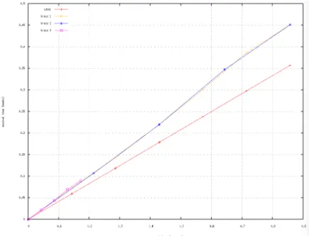
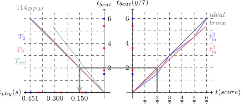
tbeat tphy(s) 2 4 6 0.150 0.300 0.451 114BP M T2 T3 Trel t(score) tbeat(y/7) 1 7 2 7 3 7 4 7 5 7 6 7 2 4 6 ideal trace t2in t3 in
Figure 18: Input traces using TIFs. From the bottom right to the bottom left, the picture presents the application of two functions (the left one is rotated to 90o to the left to take in
input the output of the first-right function). The three traces are so first shifted by the related color function and the shifted values are next translated with a tempo curve function.
and reciprocally, Honing outlines the interest of considering independently tempo curves and time-shifts for defining musical perfor-mances. They have indeed two well dis-tinct musical significance. Roughly, the first describes global continuous changes of du-rations, and the second local changes (like swing notes).
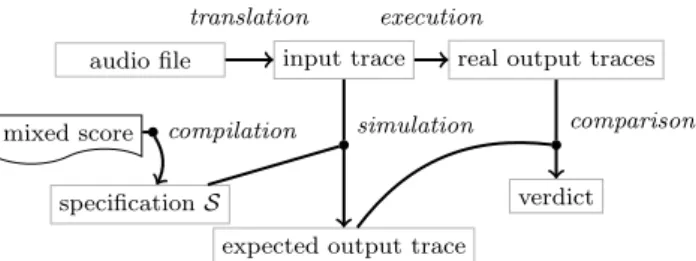
2.3.2 Generation of Inputs Traces In our MBT method, we construct input test traces using an extended TIF model that will transform (fuzz ) the ideal trace associated to the given mixed score (as defined in Sec-tion 1.4) into an artificial performance tin,
see Figure 19. More precisely, the transfor-mation applies the function f+ which mod-ifies the durations, then the tempo curve f×, and finally choose some missed events. This latter step is an addition of the models of [16, 10]. mixed score specification S ideal trace compilation input traces
expected output traces simulation
real output traces comparison verdict generation
fuzzing execution
Figure 19: Fuzz testing workflow.
Example 12. We show in Figure 18 the given input traces of the previous section with TIFs. The gray data depicts ideal values, the blue t2inand the red t3in trace. ♦ The implemented fuzzing function takes in input an ideal trace and three parameters for bounding the deviations on the time-shifts, the tempo values and the number of miss-ing notes. It generates some random values within theses limits and applies them to re-turn an input trace tin from the ideal trace.
An interesting open question in this con-text is the definition of TIFs for the genera-tion of covering test suites following criteria similar to those of Section 2.2.2.
2.3.3 Computing Expected Outputs
The above method only provides input test data traces tin. In order to compute the
cor-responding expected output traces tout and
carry out the test method described in tion 1, we still rely on the models of Sec-tion 2.1. and simulaSec-tion techniques presented in Section 2.2.3.
2.4 Testing from an audio file
We have considered a third alternative for the generation of test input traces, based on an audio recording. The developers of the IMS Antescofo use to work with sound files
mixed score specification S
audio file
compilation
input trace
expected output trace simulation
real output traces comparison verdict translation execution
Figure 20: Audio file workflow.
case c. miss nb score nb trace time (s) 0 582 1843 140 B 3 582 5718 334 6 582 6387 405
Table 1: Results for the Benchmark.
in order e.g. to analyse a specific perfor-mance that causes errors. Such sound file can be translated into an input trace simply by marking the dates of event’s onsets. We can do that manually or using softwares, e.g. Antescofo itself, which can trace the events triggered when the listening machine detects them from the audio file.
As in the previous cases, we still rely on the models of Section 2.1 and simulation tech-niques presented in Section 2.3.3 in order to compute the expected output trace tout.
3
Experiments
In this section we present the application of our MBT framework to two case studies: B, a benchmark made of hundreds of little mixed scores, covering many features of Antescofo’s DSL and EIN , a real mixed score of the piece of Einspielung by Emmanuel Nunes 3.
Each case study is processed three times, with different numbers of possible consecu-tive missing events (0, 3 and 6 events) and a bound of 5% for the variation of the duration in the interpretation of each event.
3.1 Benchmarks
We have developed a benchmark of small scores useful to the development (debugging
3http://brahms.ircam.fr/works/work/32409/
and regression tests) of the system Antescofo. It aims at covering the IUT’s DSL functional-ity and checking the reactions of the system. A script creates the IR and TA models, generates test suites (using CoVer), executes them according to the first scenario presented above (Section 1.5.1) and compares the out-come to test cases. Table 1 summarizes the results for the Benchmark B, reporting the number of traces generated by CoVer and the time taken by the whole test. Note that the number of traces increases with the number of missed events.
3.2 Einspielung
This second case study is a long real test case, for evaluating the scalability of our test method. It is composed of two extracts: the first 4 bars (22 events and 112 actions) and 14 bars (72 events and 389 actions) of the mixed score of Einspielung. Table 2 summa-rizes the results, with the number of IR loca-tions, traces and testing time for each extract. CoVer did not succeed to generate the input traces for the 14 bars extract in the case of 6 possible missed events.
3.3 Feedbacks
Despite CoVer scalability problems (that can be bypassed with other scenarios), the suites of traces generated are relevant for testing the reaction of the IUT to an exhaustive set of possible performances. Some bugs in An-tescofo were detected (as e.g. depicted in the verdict Figure 12) for specific performances, which are not easy to find manually.
We have seen that CoVer generates input test traces with minimum durations (satisfy-ing a given reachability property), and this
case c. miss locations nb trace time (s) 0 400/1394 7/35 1/24 EIN 3 518/1812 36/50 3/198
6 771/2815 67/NA 97/400
Table 2: Results of experiments on Einspielung
may cause a problem of exponential tempo acceleration described in the example t3in Sec-tion 1.5.2. Unfortunately it is impossible to change the choice of durations during the test input generation with CoVer.
Moreover Uppaal and its underlying model of timed automata networks also have some limitations. In particular, they cannot deal with multiple time-units, a feature of An-tescofo’s DSL. CoVer requires to express in extenso in E all the observable messages (with a? transitions), which causes an explosion in size of the environment model. The extension to patterns in the labels of transition (e.g. catch all symbols beginning by a) could help reducing the size of E .
Conclusion and Further Work
Thanks to an ad’hoc intermediate representa-tion for mixed scores, and a conversion into timed automata, we have developed a fully automatic offline model-based testing proce-dure applied to the interactive music system Antescofo, increasing the guarantee on reli-ability of this system. Alternative methods for the generation of test input data allow to use this test framework for different purposes, either for debugging the IMS, preparing con-certs or for assistance to composition. For the latter application, we are planing an in-tegration into the environment Ascograph for the edition of Antescofo mixed scores, with a graphical presentation of the test input and outcome.
Acknowledgments
We wish to especially thank the Uppaal’s team member for their help.
References
[1] D. A. Jaffe. Ensemble Timing in Com-puter Music. ICMC, 1983.
[2] R. Dannenberg. Music Representation: A Position Paper. ICMC, 1989.
[3] R. Alur and D. L. Dill. A theory of timed automata. Theorretical Computer Sci-ence 126:183–235, 1994.
[4] D. P. Anderson and R. Kuivila. A sys-tem for computer music performance. J-TOCS 8:56–82, 1990.
[5] J. Arias, M. Desainte-Catherine and C. Rueda. A Framework for Composi-tion, Verification and Real-Time Perfor-mance of Multimedia Interactive Scenar-ios. ACSD, 2015.
[6] J. Blom, A. Hessel, B. Jonsson and P. Pettersson. Specifying and generat-ing test cases usgenerat-ing observer automata. FATES, 2004.
[7] H. Bowman, G. Faconti, J.-P. Katoen, D. Latella and M. Massink. Automatic verification of a lip synchronisation algo-rithm using Uppaal. FMICS, 1998.
[8] A. Cont. A coupled duration-focused architecture for realtime music to score alignment. IEEE TPAMI 32(6):974–987, 2010.
[9] A. Cont, J. Echeveste, J.-L. Giavitto, F. Jacquemard. Correct automatic ac-companiment despite machine listening or human errors in antescofo. ICMC, 2012.
[10] R. B. Dannenberg. Abstract time warp-ing of compound events and signals. Comp. Music Journal 21(3):61–70, 1997.
[11] J. Echeveste, A. Cont, J.-L. Giavitto, F. Jacquemard. Operational Seman-tics of a Domain Specific Language for Real Time Musician–Computer Interac-tion. JDEDS 23(4):343–383, 2011.
[12] J. Echeveste. Un language de program-mation pour composer l’interaction mu-sicale. PhD thesis, 2015.
[13] H. Henkjan. From time to time: The representation of timing and tempo. Computer Music Journal 35(3), 2001.
[14] A. Hessel, K. G. Larsen, M. Mikucio-nis, B. Nielsen, P. Pettersson and Skou. Testing real-time systems using Uppaal. Formal Methods and Testing, Springer LNCS 4949:77–117, 2008.
[15] H. Honing. From time to time: The rep-resentation of timing and tempo. Com-puter Music Journal 25(3):50–61, 2001.
[16] H. Honing. Structure and interpretation of rhythm and timing. Dutch Journal of Music Theory 7(3):227–232, 2002.
[17] M. Krichen and S. Tripakis. Black-box conformance testing for real-time sys-tems. SPIN, Springer LNCS 2989:109– 126, 2004.
[18] N. Peters, T. Lossius and T. Place. An automated testing suite for computer music environments. SMC, 2012.
[19] C. Poncelet and F. Jacquemard. Model Based Testing of an Interactive Music System. ACM SAC , 2015.
[20] C. Poncelet and F. Jacquemard. Test Methods for Score-Based Interactive Music Systems. ICMC SMC, 2014.
[21] M. Puckette. Combining event and sig-nal processing in the max graphical pro-gramming environment. Computer Mu-sic Journal 15:68–77, 1991.
[22] M. Puckette. Pure data: Recent
progress. Third Intercollege Computer Music Festival 1–4, 1997.
[23] R. Rowe. Interactive Music Sys-tems: Machine Listening and Compos-ing. AAAI Press, 1993.