Cost of complexity : mitigating transition complexity in mixed-model assembly lines

(1)

1

Cost of Complexity:

Mitigating Transition Complexity in Mixed-Model Assembly Lines

by

Robert Addy

MEng, Naval Architecture with Ocean Engineering, University of Strathclyde and of Glasgow, 2009

Submitted to the MIT Department of Mechanical Engineering and MIT Sloan School of Management, in partial fulfillment of the requirements for the degrees of

Master of Science in Mechanical Engineering and

Master of Business Administration

in conjunction with the Leaders for Global Operations Program at the MASSACHUSETTS INSTITUTE OF TECHNOLOGY

May 2020

Signature of Author ………... MIT Department of Mechanical Engineering and Sloan School of Management May 8, 2020 Certified by ………... Sang-Gook Kim, Thesis Supervisor Professor of Mechanical Engineering Certified by ………... Steven Spear, Thesis Supervisor Senior Lecturer, MIT Sloan School of Management Accepted by ……….. Nicolas Hadjiconstantinou Chair, Mechanical Engineering Committee on Graduate Students Accepted by ………..

Maura Herson, Assistant Dean, MBA Program, MIT Sloan School of Management

(2)

2

(3)

3

Cost of Complexity:

Mitigating Transition Complexity in Mixed-Model Assembly Lines

by

Robert Addy

MEng, Naval Architecture with Ocean Engineering, University of Strathclyde and of Glasgow, 2009

Submitted to the Department of Mechanical Engineering and Sloan School of Management, on May 8, 2020 in partial fulfillment

of the requirements for the degrees of Master of Science in Mechanical Engineering and Master of Business Administration

Abstract

The Nissan Smyrna automotive assembly plant is a mixed-model production facility which currently produces six different vehicle models. This mixed-model assembly strategy enables the production level adjustment of different vehicles to match changing market demand, but it necessitates a trained workforce who are familiar with the different parts and processes required for each vehicle.

Currently, the mixed-model production process is not batched; assembly line technicians might switch between assembling different vehicles several times every hour. When a switch or ‘transition’ occurs between different models, variations in the defect rate could occur as technicians must familiarize themselves with a different set of parts and processes. This thesis identifies this confusion as the consequence of ‘transition’ complexity, which results not only from variety but also familiarity; how quickly can a new situation be recognized, and how quickly can associates remember what to do and recover the skills needed to succeed. Recommendations follow to mitigate the impact of transition complexity on associate performance, thereby improving vehicle production quality.

Transition complexity is an important factor in determining the performance of the assembly system (with respect to defect rates) and could supplement existing models of complexity measurement in assembly systems. Several mitigation measures at the assembly plant level are recommended to limit the impact of transition complexity on system performance. These measures include improvements to the offline kitting system to reduce errors such as reconfiguring the physical layout and implementing a visual error detection system. Additionally, we recommend altering the production scheduling system to ensure low volume models are produced at more regular intervals and with consistently low sequence gaps.

(4)

4

(5)

5

Acknowledgements

I would like to thank all the staff at Nissan North America for their incredible support and guidance throughout my internship at the Smyrna assembly plant. This project would not have been possible without the support and leadership of the supply chain organization and the LGO alumni at Smyrna. I extend special thanks to the following individuals for their extensive contribution to the success of this project;

Mike Steck Gabrielle Coleman

Chris Styles Grant Caldwell

Ben Shain JS Bolton

Federico Markowicz David Walker

I am very grateful for my academic advisors, Sang-Gook Kim and Steven Spear; their input, knowledge and direction throughout this project were invaluable.

Lastly, I want to express my sincere gratitude to my LGO classmates who have been a constant source of strength, humor and inspiration throughout this program and particularly during our internships. I could not have wished for a more genuine and encouraging group of people to spend a portion of my life with. You all have immeasurably enriched my life and I will never forget this journey we have taken together.

(6)

6

(7)

7

The author wishes to acknowledge the

(8)

8

(9)

9

List of Figures

Figure 1.1 - Manufacturing Quality Tradeoff Curve ... 14

Figure 2.1 - Typical Assembly Line Configuration ... 18

Figure 2.2 - Example Choice Making Process ... 20

Figure 2.3 - Diagram of Vehicle Cycle Time in a Three Model Assembly System .... 23

Figure 2.4 - Diagram of Cycle Time in Two Model Assembly System ... 24

Figure 2.5 - Diagram of Sequence Gap of 2, or 1-in-3 Assembly Rate ... 25

Figure 2.6 - Diagram of Sequence Gap of 4, or 1-in-5 Assembly Rate ... 25

Figure 3.1 - Learning Curve for Model A & B ... 31

Figure 3.2 - Sequence Gap vs Defect Rate for Model B & C ... 34

Figure 3.3 - visualization of defect rate variation across Model A-C sequence ... 36

Figure 3.4 - System Transition Complexity Relationship to Assembly Line Batch Size ... 40

Figure 4.1 - Choice Complexity Comparison Across All Models ... 42

Figure 4.2 - Choice Complexity Comparison Across Trim Levels ... 42

Figure 4.3 - Choice Complexity Comparison Model A-C ... 43

Figure 4.4 - Illustration of Transition Complexity Effect ... 44

Figure 6.1 - Part Storage Configuration in SMAL ... 56

Figure 6.2 - Off-Line Part Storage Configuration in MMAL ... 57

Figure 6.3 - Diagram of Part Picker Working Range for High Volume Model... 58

Figure 6.4 - Diagram of Part Picker Working Range for Low Volume Model ... 59

Figure 6.5 - Visualization of Kitting Errors and Production Volume, Model A-C ... 61

Figure 6.6 - Visualization of Kitting Errors Across Model A Trim Levels ... 62

Figure 6.7 - Diagram of Effect of Kitting Errors on Cycle Time ... 63

Figure 7.1 - Comparison of Model C Sequence Gap Frequency ... 67

(12)

12

List of Tables

Table 3.1 - Model A-C Comparison of Production Volume & Defect Rate... 31

Table 3.2 - Model D-F Comparison of Production Volume & Defect Rate ... 32

Table 3.3 - Effect of Preceding Vehicle on Model A Defect Rate ... 35

Table 3.4 - Comparison of Designed Cycle Time... 35

Table 3.5 - Effect of Preceding Vehicle on Model D Defect Rate ... 37

Table 3.6 - Comparison Model A-C defect rate and number of parts... 37

Table 3.7 - Comparison Model D-F defect rate and number of parts ... 38

Table 5.1 - Rating average of complexity drivers in the flexible assembly system [9] 47 Table 6.1 - Summary of Kitting Errors for Model A-C ... 60

Table 7.1 - Summary of Model A-C Defect Rates for Second Production Period ... 65

Table 7.2 - Effect of Preceding Vehicle on Model A Defect Rate in Second Production Period ... 66

List of Equations

Equation 2-1 - Mean Choice Reaction Time ………... 21

Equation 2-2 - Choice Complexity (Information Entropy) .……… 22

Equation 4-1 - Choice Complexity Equation ………41

List of Acronyms

MMAL Mixed Model Assembly Line SMAL Single Model Assembly Line FMS Flexible Manufacturing System NNA Nissan North America

OEM Original Equipment Manufacturer JIT Just-In-Time

SUV Sports Utility Vehicle

(13)

13

Chapter 1 Introduction

This thesis aims to identify the quality implications of manufacturing a range of different products in a modern mixed-model automotive assembly system. This will allow for improvements in the design of such systems, and it will help the company understand the quality impact of rationalizing its product offerings. This chapter will present the problem statement and motivation to address it.

1.1 Problem Statement

As a global automotive company, Nissan Motor Co. Ltd., offers a range of automobiles to different markets and market segments globally. As is typical in the competitive automotive industry, there is a desire to leverage the firm’s economies of scope by offering a vehicle in every market segment, and each segment is commonly offered a choice of propulsion technology, from traditional internal-combustion to hybrid and electric drivetrains.

To remain competitive, a modern automotive Original Equipment Manufacturers (OEM) must understand the tradeoffs that exist between different competitive dimensions. As they operate in a mature market, competing firms in the automotive industry compete on multiple dimensions, including i) cost, ii) product choice & variety, and iii) differentiation through leadership in manufacturing (i.e. quality), brand and design [1]. These dimensions are not necessarily complementary, and this study aims to identify mechanisms of interaction that exist between offering greater product choice & variety to consumers and ensuring high manufacturing quality of these products.

We can imagine that a tradeoff exists between product choice & variety and manufacturing quality. If product choice & variety is zero, we expect manufacturing quality is maximized, as only product is manufactured in a perfectly repeatable process.

(14)

14

Conversely, if product choice & variety is high, we expect low manufacturing quality due to the difficulties involved in manufacturing a wide variety of products. The tradeoff between these two dimensions is shown in Figure 1.1 as a convex curve, and if transition complexity can be successfully mitigated in the mixed-model process, the tradeoff curve can move to the right, where for a fixed level of product choice & variety, we can now expect a higher level of manufacturing quality.

Figure 1.1 - Manufacturing Quality Tradeoff Curve

1.2 Project Motivation

The Nissan Smyrna automotive assembly plant has been configured to support the Nissan Flexible Manufacturing System (FMS) to enable the production of a wider variety of vehicles from the same plant. The Smyrna plant is a mixed-model facility which currently produces six different vehicles and the variants within those vehicle types. While this system allows the firm to adjust production levels of each vehicle to better match market demand, it poses challenges from a manufacturing perspective, where quality levels across the different vehicles may vary due to dissimilar production volumes. Maintaining high quality level in vehicles with lower production volumes is difficult as assembly line technicians will naturally have lower familiarity with products that are built less often.

Offering a high-quality product is important to maintaining customer loyalty and trust in an OEM’s brand, and it has been identified as the most important factor influencing a consumer’s purchasing decision [2] . Nissan has been consistently ranked by JD Power as having above average quality among automotive brands in the US Initial Quality Study [3]

Product choice & variety Manufacturing Quality Tradeoff curve if Transition Complexity is mitigated. Existing Tradeoff Curve In cr ea se Increase

(15)

15

and the firm maintains high product quality objectives within the corporate objective of ‘operational excellence’ contained within the “Nissan M.O.V.E. to 2022” corporate plan (Nissan 2017).

1.3 Project Objective

Since the consumer market demands a product variety and given that there are clear reasons for a single assembly facility to be able to build such a variety of model to adjust for demand, we are seeking a preferential policy for sequencing production that provides the variety the market needs while accounting for switching costs between one model and the next.

Currently, the mixed-model production process is not batched; assembly line workers might switch between assembling different vehicles several times every hour. We can think of the mixed-model production process as having a batch size of one; there could be a switch to a different model after every vehicle. When a switch (or ‘transition’) between different models occurs, variations in the defect rate occur as workers must familiarize themselves with a different set of parts and processes required for the next model on the assembly line.

Observation of the defect data has revealed increased defect rates after transitioning between certain models, which we propose is a direct result of the transition complexity in the mixed-model assembly system. The objective of this study is to define and quantify this ‘transition’ complexity and recommend measures to mitigate the impact of ‘transition’ complexity on vehicle production quality.

(16)

16

Chapter 2 Background

2.1 Nissan Smyrna Assembly Plant

Nissan North America (NNA) is a subsidiary of Nissan Motor Ltd (NML), the publicly traded Japanese auto maker, headquartered in Yokohama. Nissan North America (NNA) manufactures and distributes a wide range of vehicle types (including cars, SUVs, trucks and light commercial vehicles) under the Nissan and Infiniti brands. NNA operates three non-unionized manufacturing and assembly facilities: vehicle stamping and assembly plants in Smyrna, Tennessee and Canton, Mississippi, and a powertrain plant in Decherd, Tennessee.

Established in 1983, the Nissan Smyrna assembly plant is the highest-volume automotive assembly plant in North America, with the capacity to produce 640,000 vehicles annually [5]. The plant represents a $7.1 billion investment for Nissan, and it has been continually upgraded with the latest technology since its initial construction. The Smyrna plant currently produces the Nissan Altima, Nissan Rogue, Nissan Pathfinder, Nissan Maxima, Nissan Leaf and Infiniti QX60.

The plant is divided into 3 main areas; Body & Stamping, Paint and Trim & Chassis. The Body & Stamping and Paint areas of the plant are highly automated and very few parts of the vehicles are installed in these areas. This study will focus on quality outcomes in the Trim & Chassis area of the assembly plant. This area of the plant assembles the vast majority of the parts in each vehicle and almost all of the assembly work is performed manually by skilled technicians at stations on the assembly line, hence human factors are an important consideration in this area of the plant.

(17)

17

2.2 General Plant Configuration

The Nissan Smyrna plant currently assembles six models, with three models dedicated to each of two assembly lines in the Trim & Chassis area.. It is not possible to switch between lines, each group of three models is dedicated to a single line, generally for a whole year. This partitioning of models to specific lines is due to the specialized equipment required to assemble different types of vehicle and differences in assembly sequence.

For example, if sales of Model A, B & C turn out to be very low, but sales of Models D, E & F are very high, the plant cannot easily change to having both assembly lines build Model D, E & F, such a change might require several weeks of upgrade and modification work. SUV’s are physically larger than sedans, so an assembly line configured for SUV’s would have equipment that can handle the larger and heavier components such as doors, sunroof panels and engines, whereas a sedan assembly line may not be configured to deal with these components.

Each assembly line has several segments (which can be thought of as stations), and each segment has a specific ‘kit-cart’ of parts delivered to the assembly line by an autonomous guided vehicle (AGV) for the line technicians to install. The vehicles move continuously through the line segments at a fixed-speed on a large conveyor, and new kit-carts are brought to the assembly line at the beginning of each segment. The kit-carts move at the same speed as the vehicles on the conveyor, allowing the line technicians to move easily back and forth between the vehicle and the kit-cart.

Each ‘kit-cart’ is specific to a single vehicle, and they are delivered in a sequence corresponding to the sequence of vehicles on the assembly line. The ‘kit-cart’ of parts is manually pre-assembled in a dedicated ‘kitting area’ which is an in-plant part storage area. These areas utilize pick-to-light systems and instructional displays to ensure the correct parts are chosen.

The ‘kitting area’ for each line segment will hold most of the parts required to assemble the three different models (and variants) on that line segment. The ‘kitting area’ could store many thousands of parts and only a few tens or hundreds are chosen for the assembly tasks

(18)

18

on a line segment. The line technician will install all parts in the ‘kit-cart’ into the vehicle, which eliminates the selection aspect of the ‘choice complexity’ on the assembly line.

Refer to Figure 2.1 for a diagram of the typical assembly line configuration, showing two-line segments A & B;

Figure 2.1 - Typical Assembly Line Configuration

The ‘kit-cart’ travels along the assembly line with the vehicle being assembled, they are removed at the end of a line segment, sent back through the relevant ‘kitting area’ to be re-stocked with specific parts for the next vehicle in the sequence, and then sent back to the start of the assemble line segment, in a continuous loop.

In this assembly line configuration, line technicians are assigned to a specific line segment or ‘zone’, which enables specialization on a group of related tasks, such as powertrain installation, or interior trim fitting.

2.3 Mixed-Model Production

Nissan North America (NNA) has configured the Smyrna, TN, and Canton, MS, plants to operate with a mixed-model assembly process, which enables flexibility in production

➔ ➔ Assembly Line Segment ‘A’ ➔

  Assembly Line Segment ‘B’ 

Kitting Area ‘A’

Vehicle Enters Kit-cart Kit-cart Kitting Area ‘B’ Kit-cart Kit-cart Continues to Segment ‘C’

(19)

19

volumes, as the build volume of different vehicles can flex up or down to better match demand throughout the year. This operating strategy also enables Nissan to be produce a greater range of vehicles at each plant, thus allowing the company to offer more vehicles while controlling capital expenditure on fixed assets.

This is a useful production system for low-volume but high-variety products, provided there is adequate similarity between the products, as the switch-over cost between models should be small. Mixed-model production ensures a more continuous flow of each model, and it generally reduces the in-process and finished goods inventory [6]. A mixed-model production system is one of the foundations for applying a Just-In-Time (JIT) supply chain system, as it provides smoother production, compared to batch processing.

2.4 Overview of Current Mixed-Model Sequencing Methodology

The assembly line system at Nissan Smyrna allows for multiple models to be built on a single assembly line, with an effective batch size of one vehicle. Depending on demand for each type of vehicle, assembly line technicians could find themselves assembling five sedans in a row, or they may switch from a sedan to a compact and then to a sports utility vehicle (SUV).

The dominant consideration which affects mixed-model scheduling is ‘capacity balancing’, where the production schedule of different vehicles is created based on the varying cycle time for the build process of each vehicle. For example, a more complex (higher or premium trim level) vehicle may take slightly longer than average to assemble due to the increased feature content, so the scheduling system ensures that this vehicle is not built in batches and is instead mixed with other vehicles that take slightly less time than average to assemble.

This capacity balancing allows line technicians to fall behind when assembling more complex vehicles and then ‘catch up’ when assembling simpler vehicles. As the assembly line is split into multiple sections, ‘capacity balancing’ is important to ensure that technicians can complete the tasks required within their line segment or ‘zone’, otherwise

(20)

20

they may have to stop the line to complete the work, as they cannot move with the vehicle into the next zone.

A greater volume of low and middle trim level vehicles are typically sold than higher (premium) trim levels, due to the reduced price of lower and middle trim level vehicles capturing a larger market of potential consumers. Consequently, premium trim vehicles with a batch size of one are mixed into larger batches of middle and low trim level vehicles. Therefore, the higher (premium) trim level vehicles having a higher probability of increased transition complexity.

2.4.1 Choice Making and the Hick-Hyman Law

Each vehicle model and trim level have a variable part content, depending on the feature content of the vehicle, for example, premium trim levels could have additional parts for an enhanced entertainment system, or additional electrical wiring for heated seats. At the start of each assembly line segment, a kit-cart which is specific to each vehicle, arrives at side of the assembly line. Even though the kit-cart has been compiled in an offline part storage area, the line technicians must make a series of correct choices; i) select the correct parts, ii) in the correct order, and iii) select the correct tools (or fixtures) to complete the work in their segment. Each of these choices requires time to be made correctly.

Figure 2.2 - Example Choice Making Process

Sedan _SUV

Sedan Kit-Cart (8 parts)

SUV Kit-Cart (12 parts)

(21)

21

To visualize the choice making process on the assembly line, we refer to Figure 2.2 above. The sedan kit-cart has 8 parts to be installed, each part represented by the black circles, and half of these parts requires a different tool choice for installation. Thus, the sedan requires twelve choices; eight part choices plus four tool choices. The SUV kit-cart has twelve parts, each part represented by the black diamond in the kit-cart, and all of those parts require a different tool choice for installation. The SUV requires twenty-four choices, twelve part choices plus twelve tool choices. In this example, the SUV requires double the choices of the sedan, and hence the cycle time for the SUV will be longer on this line segment.

In reality, at the Smyrna plant, each kit-cart could hold tens of parts, and each part may require the correct fixtures to be chosen (i.e. multiple screws or bolts) in addition to the correct tool choice (i.e. torque wrench). Therefore, each assembly line segment will require hundreds of correct choices to be made.

If a greater number of parts than average arrives in a kit-cart, we would expect the line technician to take longer to assemble these parts, as there are simply more parts to install, and each choice requires time to be made.

The variation of cycle time, which is proportional to the vehicle part content, is a consequence of human choice-making activities which obeys the Hick-Hyman Law [7]. The Hick-Hyman law states that average choice reaction time (RT) is linearly proportional to the logarithm of the number of alternatives, if all alternatives are equal. The Hick-Hyman law is generalized as follows;

𝑀𝑒𝑎𝑛 𝐶ℎ𝑜𝑖𝑐𝑒 𝑅𝑇 = 𝑎 + 𝑏𝐻 (2-1)

Marin et al. define Choice complexity as the average uncertainty or randomness in a choice process, which can be described by a function H (representing information entropy) in the following form [7];

(22)

22

𝐻(𝑋) = 𝐻(𝑝₁, 𝑝₂, … , 𝑝_𝑚) = −𝐶 ∑ 𝑝_𝑚log 𝑝_𝑚

𝑀 𝑚=1

(2-2) Where pm is the probability of a choice taking the mth outcome. Here H is exactly equal

to [ log2𝑛], where 𝑛 is the number of alternatives (i.e. choices). This arises as all of the pm’s are equal, since the choice process is independent and identically distributed (iid) and

all alternatives are equally likely to occur. The variables a and b are constants which must be determined empirically by fitting a line to measured data. These variables will account for characteristics of the choice process, such as difficulty or lack of familiarity.

While the cycle time (i.e. assembly time) of vehicles assembled in the Trim & Chassis section of the Smyrna plant is based on actual assembly experience, it is nevertheless a useful result that cycle time obeys the Hick-Hyman law. This is due to the vast majority of the processes in the Trim & Chassis area being manual (i.e. human) choice processes. We therefore know that a reduction in the number of choices at each station will result in a lower cycle time.

In additional to the variable part content mentioned above, each vehicle model may have a different build sequence, so the type of parts delivered to the assembly line in the kit-cart will be different for each vehicle, which increases the difficulty of the choice making process. Equally, when assembling low-volume models the line technician is less familiar with the parts and tools required to install them, further increasing the time taken. Variables

a and b can describe the choice making difficulty of the process. 2.4.2 Variation of Cycle Time

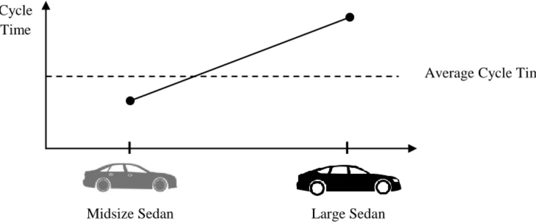
The variation of cycle time with vehicle is shown in Figure 2.3 below. The part content (i.e. the assembly jobs required) for each vehicle drives the cycle time requirement, i.e. vehicle with more parts have a higher cycle time. Therefore, we would expect vehicles with a higher cycle time to have a higher defect rate due to higher entropy and the increased stress placed upon line technicians of having assemble a more complex vehicle in an allotted time.

(23)

23

Figure 2.3 - Diagram of Vehicle Cycle Time in a Three Model Assembly System If these three vehicles are built on the same line, the expected build quantity will have to be matched with the cycle time. The assembly line will be well balanced in terms of cycle time if the build quantity of the compact and large sedan are equal, and therefore will cancel each other out. If the midsize sedan is the dominant model, then the assembly line can tolerate un-balanced production of the compact sedan and large premium sedan and the overall average cycle time will be close to the average. In this example, variation in cycle time

For a mixed-model assembly line with only two vehicles as shown in Figure 2.4 below, the average cycle time would be balanced considering the production volume of the two vehicles. In the below figure, if the midsize sedan is 75% of the production volume, and the large premium sedan is 25%, then the average cycle time on the assembly line will be 25% greater than that of the midsize sedan, i.e. the cycle time changes in proportion to the difference in production volume.

Compact Sedan Midsize Sedan Cycle

Time

Average Cycle Time

(24)

24

Figure 2.4 - Diagram of Cycle Time in Two Model Assembly System

2.5 Mixed-Model Sequencing Constraints

The current mixed-model sequencing constraints relate to capacity balancing, as described above. The sequencing system is constrained by how frequently a vehicle with a longer than average cycle time can be produced on the assembly line. For example, if a vehicle has a sunroof, there are some additional processes which must be carried out, compared to a vehicle without a sunroof. These additional processes could include lifting a glass panel above the vehicle into place, connecting additional electrical components to control the sunroof and function testing all of these additional components. As this vehicle with a sunroof has a longer cycle time, the vehicle before or after it on the assembly line must take less than the average cycle time in order for the line workers to ‘catch up’ the time and maintain the target production level. Similar constraints apply to a variety of other vehicle options, as well as entire vehicle models.

A high-end vehicle model may have relatively low forecasted production volume, where on average, it is produced at a rate of 1-in-10 vehicles. It may additionally be subject to a scheduling constraint where it cannot be assembled at a rate greater than 1-in-5 vehicles due to the higher than average cycle time to assemble this vehicle While on average this constraint appears to be non-limiting, if the plant intends to increase the production rate of the vehicle, it can only increase up this scheduling constraint to maintain capacity balance.

Cycle Time

Average Cycle Time

Large Sedan Midsize Sedan

(25)

25

The constraints currently defined in the scheduling system define the maximum frequency with which a model can be produced, but there are no minimum constraints used, for example, there are no constraints requiring a minimum production rate of 1-in-20.

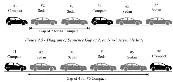
2.5.1 Definition of Sequence Gap

In the mixed-model assembly process, the ‘gap’ between two models of the same vehicle is variable. The gap preceding each vehicle was used to examine the relationship between the sequence gap of an individual vehicle and build quality. Figure 2.5 below illustrates a sequence gap of 2 for Compact vehicle #4, corresponding to a assembly rate of 1-in-3. Figure 2.6 illustrates a sequence gap of 4 for Compact vehicle #6, corresponding to an assembly rate of 1-in-5. In Figure 2.5, the #5 sedan has a sequence gap of 1 as it was preceded by a compact model, and #6 sedan has a sequence gap of 0, as it was preceded by another sedan.

Figure 2.5 - Diagram of Sequence Gap of 2, or 1-in-3 Assembly Rate

Figure 2.6 - Diagram of Sequence Gap of 4, or 1-in-5 Assembly Rate

2.6 Overview of Vehicle Models and Variants

A modern automotive OEM could offer hundreds of different vehicles to consumers. For example, each model could be offered with 2 drivetrain options; front-wheel drive and all-wheel drive. Each of these drivetrains could be offered with solid roof or sunroof, and

Gap of 2 for #4 Compact = 2 #1 Compact #2 Sedan #3 Sedan #5 Sedan #6 Sedan #4 Compact

Gap of 4 for #6 Compact = 4 #1 Compact #2 Sedan #3 Sedan #4 Sedan #5 Sedan #6 Compact

(26)

26

all of these options can be offered in perhaps 5 trim different trim levels, with multiple variants within each trim level containing different feature packages and varying interior finishes. This thesis will not examine models down to this detail, as it is often too granular to produce meaningful results due to ever decreasing sample sizes as we get more specific. This study will concentrate on comparing defect data at the model level and trim level within each model.

2.6.1 General Nomenclature

Within this thesis, the models assembled at the Smyrna plant shall be denoted as Model A-C and Models D-F, where each group of models is assembled on a separate assembly line. The various trim levels within each model denoted as 1-5. Where the term Model A is used, it includes all the trim levels within the model. If a specific trim level is referred to, it will be denoted as, for example A-1, which denotes Model A, trim 1.

(27)

27

Chapter 3 Initial Observations from Defect Data

This chapter outlines several initial observations from the defect data. Initial analysis of the data is undertaken to understand the general systematic behavior of the assembly system and determine if the assembly plant staff’s observations of the system’s behavior are substantiated.

The defect rates of Models A-C are compared to Models D-F, where these two groups of vehicles are produced on different lines and with differing production volumes. Within the grouping of Model A, B & C on one assembly line, it is known that Models A & B share a large number of common parts and assembly processes, while Model C has significantly different parts and processes compared to Model A & B.

Within the grouping of Model D, E & F, Models E & F share a large number of common parts and processes, while Model D differs in terms of parts, it shares common processes with Models E & F.

3.1 Overview of Data Sources

This study utilizes data generated from the in-plant defect logging system at the Smyrna assembly plant along with manufacturing information for each vehicle. Here the term ’defect’ is used generally to describe any unsatisfactory condition logged in the system during assembly, which will then be rectified prior to completion.

3.1.1 Defining Relevant Defect Data

For the purposes of this study, defect data includes all issues logged in the system within the ‘Trim & Chassis’ area of the plant. This data is logged immediately after a defect is detected at the side of the assembly line in dedicated computer terminals. Defects detected and rectified in the Body & Stamping and Paint sections of the plant are not considered

(28)

28

part of this study, as our point of interest is how part complexity affects defect rates. Defect data for vehicles which are already in-service (i.e. from customers or end-users) is not considered in this study, such data would include part defects originating with suppliers and defects resulting from a variety of external factors which are difficult to differentiate.

3.1.2 Design Data – Bill of Materials, numbers of parts being assembled

For vehicles assembled at the Smyrna plant (i.e. specific model, trim & variant), the bill of materials was extracted, which provided a complete list of the parts (and sub-assemblies) which are assembled at the plant. For example, a headlamp sub-assembly might consist of many individual parts, but this would be considered a single item in the Smyrna plant, equivalent to a part. The vehicle models produced at Smyrna are offered in a variety of trim levels, each targeted at a different market segment. Each of these trim levels is then offered in multiple variants, each with a variable part content.

3.1.3 Defect (Quality) Data from In-plant Systems.

Defect data from the Trim & Chassis part of the assembly plant was extracted from the in-plant defect logging system for a 12-month the period in 2018-19. The defects were logged during in-plant assembly processes and rectified during or after assembly. The defects logged could be missing parts, parts not installed according to specifications, or even dirty parts which must be cleaned.

The defects recorded for each vehicle are normalized by dividing by the number of parts within the vehicle and dividing by 1,000, so that a defect rate per 1000 parts is used for comparison across vehicles. We can expect a vehicle with more parts to have a greater defect rate, as there are more installation operations to perform, each of which can be correct or incorrect. Defect rates in this study are normalized with respect the dominant vehicle on the assembly line, i.e. the vehicle with the greatest production volume will have a defect rate of 1.0.

3.1.4 Scheduling Data for Build Sequence

The actual build sequence of vehicles in Trim & Chassis part of the plant was used. The actual build sequence of vehicles in each section of the plant varies, due to the designed buffer areas where finished products from one part of the plant are held for quality

(29)

29

inspection before being released to the next section, thus the sequence in which vehicles are assembled in Body & Stamping is different from the sequence in the Trim & Chassis section.

3.1.5 Data Selection for Analysis

During the 12-month period for which data was extracted, there are many minor and major model launches, where a particular model may have styling updates (minor launch), or a whole new vehicle may be launched (major launch). After each minor or major model launch, there will be a learning curve where the assembly line technicians must become familiar with the updated parts and assembly sequence for the vehicle.

The dramatic learning curve associated with a new model launch can be seen in Figure 1 above; the defect rates reaches a steady state after approx. 4 months of production. The objective of this study was to examine the effect of steady-state processes on defect rates, so two periods of approximately 6-8 weeks were selected for analysis, where the defect rate was relatively constant for all vehicles, and no observable learning curve existed.

3.1.6 Combining the Data

In the current mixed-model production system, defect rates for each vehicle are tracked to enable root-cause analysis of defects identified during the assembly process. This defect tracking is performed for each vehicle in isolation, and the effect of build sequence is not accounted for when examining defect rates. The different vehicles built on the same assembly line are assumed to be sufficiently similar such that the switching cost of transitioning between different vehicles is zero. This assumption is one of the core assumptions of the mixed-model sequencing system [6]

To quantify this switching cost between models, the defect data has been examined from the point of view of sequence, i.e. what influence, if any, does one vehicle have on the following vehicle.

3.1.7 Vehicles for non-US markets

The Smyrna plant produces vehicles designed for a range of markets outside the US domestic market, many of which have specific parts required by local market regulations.

(30)

30

The different part content of these vehicles means that the build sequence is often modified to balance the jobs over the assembly process. Additionally, the line technicians are not familiar with many of these specific parts, due to the low production volumes of the export vehicles leading to potentially higher defect rates for a vehicle model. As this increase in defect rate is attributable to specific parts in export model, rather than the normal plant processes, these export vehicles are excluded from the data set.

3.2 Learning Curve in Assembly

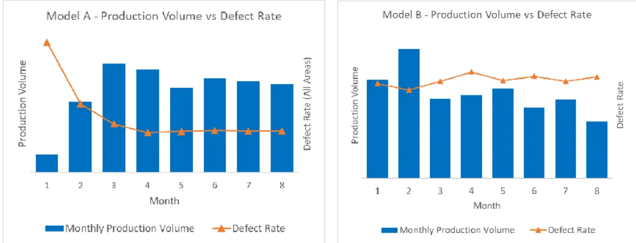
The full 12-month defect data for a high-volume vehicle Model A which was a major model introduction during the period analyzed is shown below. After the start of production (SOP), the defect rate declines rapidly and remains largely flat, even with fluctuations in monthly production volume. This indicates that there is a significant learning effect, where the plant workforce needs to assemble a certain number of units in order to reach maximum level of familiarity (and competency) with the vehicle model.

For this high-volume vehicle, Model A, we plot defect rates for each of the five trim levels and find a strong relationship between the trim levels, despite high variability in the production volume. This indicates a combined learning effect which is independent of the production volume for each trim level and is dictated by the combined production volume for all variants. This can be explained by the fact that most parts across the variants are similar, and even where parts may differ, the general assembly processes do not.

Vehicles with lower production volumes do not reach this flat level of defect rates, as they are not being assembled frequently enough for the workforce to reach this maximum level of familiarity (and competency) with the vehicle’s parts & processes. We observe that the defect rate is negatively correlated to monthly production volume, which can be thought of as the familiarity level of the workforce reducing gradually over time. Figure 3.1 below shows charts of monthly build volume plotted with the trend of average defect rate for Model A & B (Model C is not shown but displays a trend similar to Model B).

(31)

31

Figure 3.1 - Learning Curve for Model A & B

Due to the learning curve observed for Model A, data for months 1-3 will not be considered as part of this study, as they are not the result of a steady-state system.

3.3 Defect Rates on Each Assembly Line

For a steady state production period, we can compare production volume, defect rate and sequence gap for Model A-C.

Table 3.1 - Model A-C Comparison of Production Volume & Defect Rate Vehicle Model Production Volume Normalized Overall Defect Rate Average Sequence Gap Between Models

Model A 75% 1.00 0.3

Model B 20% 1.40 4.2

Model C 5% 2.82 19.7

Referring to Table 3.1, we can see that the production volumes for Model B & C are low, and thus the elevated defect rates could be the result of reduced familiarity among workforce with these models. Model A & B share many common parts and assembly processes, while Model C differs greatly in parts & assembly compared to Model A & B. The sequence data for Model A-C does not display a regular repeating production pattern.

(32)

32

The production volume, defect rate and sequence gap for Model D-F are given in Table 3.2 below. There is less variation in the defect rates between the three models, and difference in the production volume is also reduced. In this case, Model E & F share a large number of common parts and similar assembly processes, and they share only a small number of parts with Model D. The sequence data for Model D-F shows that in general, this assembly line follows a dominant repeating pattern of D-E-D-F.

Table 3.2 - Model D-F Comparison of Production Volume & Defect Rate Vehicle Model Production Volume Normalized Overall Defect Rate Average Sequence Gap Between Models

Model D 51% 1.00 1.0

Model E 26% 1.11 2.8

Model F 23% 1.20 3.5

When we compare the defect rates of Model A-C and Model D-F, factors such as the vehicle characteristics and how the commonality of assembly processes with the dominant model on the assembly line are important.

Model E & F share a common product architecture and have a large proportion of common parts and therefore this group of three vehicles can be approximated as one assembly line switching between two models, which indicates why the normalized defect rates are relatively close. The variance in the defect rate can be reasonably explained by Models E & F having a higher part content and cycle time than Model D. That is, the line technicians assembling Models E & F will have to install more parts in the same amount of time, and therefore we might expect higher rates of defects due to two factors; i) greater number of choices, and ii) greater stress to complete the job in the allotted time.

Model A & B share a common platform and many common parts, yet the normalized defect rate of 1.40 is greater than that of Model E & F, despite similar production volumes. The lack of repeating production pattern for Model A-C could explain the greater variance in defect rates from the dominant model. The product architecture of Model C is

(33)

33

significantly different from Model A & B, coupled with low production volume of 5% could elucidate the high normalized defect rate of 2.82.

3.4 Effect of Sequence Gap

The apparent relationship between production volume and defect rate indicates that we might expect the defect rate of an individual low-volume vehicle to be correlated with the sequence gap between low-volume vehicles. That’s is, if a low-volume vehicle is built with a frequency of 1-in-10, we would expect higher defect rates than if it was built with a frequency of 1-in-5. This leads us to expect that the sequence ‘gap’ is an important factor in determining vehicle quality in the mixed-model production process, where the ‘gap’ is defined as the number of different vehicles between two vehicles of the same model.

Increasing the ‘gap’ between two models of the same type, the line workers become less familiar with the operations and parts required for this vehicle and therefore the defect rate could rise. In the case of Model A, we expect that this model is built so frequently that the defect rate has reduced to the lowest steady-state rate, as worker familiarity with this model has reached a maximum level.

Generally, Model A has a gap less than or equal to 1 as it is the dominant model, while Model B & C have gaps ranging from 1 to over 50, as they are slotted into the production process. Only US domestic models have been analyzed, the export models have been excluded from this analysis, as they have a significant number of different parts which will affect the defect rates since assembly workers are less familiar with these parts.

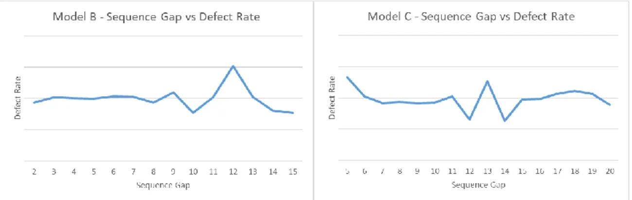
3.4.1 Analysis of Sequence Gap

Plots of the average defect rate against the sequence gap for Model B & C are shown in Figure 3.2 below and shows no strong relationship between these two factors at the individual vehicle level. For Model B, 95% of the vehicles had a sequence gap between 1 and 9. The data plot was truncated at sequence gap of 15, due to there being a small number of data points at higher values of sequence gap. For Model C, 69% of the vehicles had a sequence gap between 1 and 20. The data plot was truncated at sequence gap of 20, due to

(34)

34

the low number of data points above this value. No reliable relationship between sequence gap and defects rate was found.

Figure 3.2 - Sequence Gap vs Defect Rate for Model B & C

The plots in Figure 3.2 above show that the vehicle-specific sequence gap is not an important factor in determining the defect rate in the mixed-model process. Although there is a link between the monthly production volume and the defect rate (as shown in Figure 3.1), the rate at which workers gain or lose familiarity with any particular vehicle model appears to be slow; lower build volumes for a period of weeks or months will contribute to greater defect rates, but these are gradual declines over time. Therefore, production volume fluctuation produces defect rate variation at the monthly level, but not at the daily (or hourly) level.

3.5 Effect of Preceding Vehicle on Defect Rates

The sequence gap does not appear to an important factor in determining defect rates of individual vehicles, and therefore the switch between different vehicle models is investigated to establish its contribution to defect rates. Both Model B & C are almost always preceded by Model A due to the production volume mix of the period analyzed, and we expect that this switch or ‘transition’ between different models contributes to the defect rates of Models B & C being greater than Model A.

Two-thirds of the Model A vehicles are preceded by other Model A vehicles and so the average complexity of the switch (or ‘transition) for Model A is lower, which contributes to the reduced defect rates for Model A vehicles, along with the greater degree of workforce familiarity with this vehicle.

(35)

35

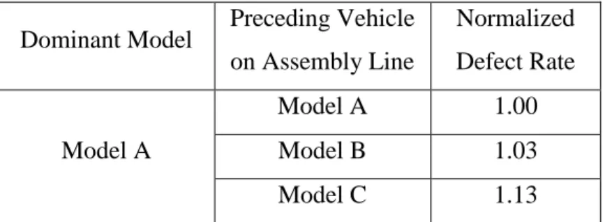
Table 3.3 - Effect of Preceding Vehicle on Model A Defect Rate

Dominant Model Preceding Vehicle on Assembly Line Normalized Defect Rate Model A Model A 1.00 Model B 1.03 Model C 1.13

The results in Table 3.3 above show that the preceding vehicle on the assembly line has an effect on defect rate. If a Model A vehicle is preceded by another Model A vehicle, the normalized defect rate is 1.00, but if a Model A vehicle is preceded by a Model C vehicle, the normalized defect rate is 1.13 (i.e. a 13% higher defect rate). In this case that Model A & B share a greater number of common parts than Model C does with either A or B. Since Model B & C are always preceded by a Model A vehicle, due to the production volume mix, this comparison for those vehicles is not possible. This data only includes US domestic vehicles, and vehicles preceded by other US domestic vehicles.

Table 3.4 - Comparison of Designed Cycle Time

Vehicle Model Designed Cycle Time

Model A Average

Model B Above Average Model C Below Average

Table 3.4 above compares the designed cycle time for each vehicle, which is a summation of the time to perform each individual assembly task for each vehicle. This method of calculation essentially follows the Hick-Hyman Law, as cycle time is proportional to the number of parts,

The increase in Model A defect rate following a Model C vehicle occurs despite Model C having a lower cycle time than Model A, and we would therefore expect that the line

(36)

36

technicians would have excess time to assemble the Model A vehicle. It appears from this data that this is not the case, and actually the Model C vehicle takes longer to assemble than predicted, thereby reducing the time available for assembly of the Model A vehicle and causing a higher defect rate in those vehicles. The variation in defect rate is shown visually in Figure 3.3 below.

Figure 3.3 - visualization of defect rate variation across Model A-C sequence

For Model D-F the transition between models has a minor effect on defect rates, which could be a consequence of the regular repeating production sequence on this line, and because of the greater extent of part and process sharing across these three models. This combination of factors will reduce the transition complexity. In Table 3.5 below, Model D preceding another Model D vehicle appears to elevate the defect rate, however this is due to this transition occurring only where low-volume premium trim levels of Model D are produced, and therefore we have a higher part content combined with line technicians being less familiar with the additional part content of these vehicles. This data is also collected from 6-8 weeks of production data, not over a whole year, and therefore the effect of these transitions on defect rates at other points during the year could vary.

Model A

Model A Model C Model A Model A

1.0 _1.0 2.82 1.0 1.13 D ef ec t Rate

(37)

37

Table 3.5 - Effect of Preceding Vehicle on Model D Defect Rate

Dominant Model Preceding Vehicle on Assembly Line Percentage of Transition Normalized Defect Rate Model D Model D 14% 1.04 Model E 46% 1.02 Model F 40% 1.00

3.6 Effect of Number of Parts on Defect Rates

Referring back to the Hick-Hyman Law (Section 2.4.1), we would expect vehicles with a lower number of parts to have lower defect rates, due to the reduced number of choices (i.e. complexity) required for their assembly. In the below tables, the number of parts in each model was averaged across all trim levels and normalized to a baseline of 1,000 parts for the dominant model.

Comparing Model A-C in Table 3.6, we observe that defect rate and number of parts for Model B are positively correlated, while for Model C they are not. This suggests that Model C suffers from a high level of transition complexity, which contributes to the elevated defect rates.

Table 3.6 - Comparison Model A-C defect rate and number of parts Vehicle Model Production Volume Normalized Overall Defect Rate Normalized Total Number of Parts Model A 75% 1.00 1,000 Model B 20% 1.40 1,066 Model C 5% 2.82 938

We observe in Table 3.7 below that defect rate and number of parts for Models D-F are positively correlated, suggesting that transition complexity between these models is low.

(38)

38

Table 3.7 - Comparison Model D-F defect rate and number of parts Vehicle Model Production Volume Normalized Overall Defect Rate Normalized Total Number of Parts Model D 51% 1.00 1,000 Model E 26% 1.11 1,181 Model F 23% 1.20 1,243

3.7 Transition Complexity Hypothesis

Comparing Model A-C and Model D-F defect rate variations over different transitions leads us to the hypothesis that transitions with a high degree of difference (i.e. magnitude of difference in familiarity, parts & processes) between the two vehicles can cause elevated defect rates. This suggests that models built on a common line should be as similar as possible, thereby reducing the Transition Complexity of the system and hence the defect rates.

Switching between two vehicles in a mixed-model assembly process can be thought of as transitioning from assembly of one complex product to another, and thus the term ‘transition complexity’ shall be used to describe this difference. The difficulty of the transition from one vehicle to another is determined by the difference in multiple factors across the vehicles, all of which increase the mental burden placed on line technicians performing the assembly tasks; i) the familiarity of the line technicians with each vehicle, ii) the difference in the part content, iii) the difference in part assembly sequence, and iv) the difference in assembly processes (tools, fixtures used, etc).

The cycle time calculated for each model should in fact account for the transition complexity that exists when switching between models on the assembly line.

(39)

39

3.8 Description of Factors Influencing Transition Complexity

3.8.1 Production Frequency

Increasing the production frequency of a particular model results in the plant’s workforce having a greater level of familiarity with the parts & processes required for assembly, thus reducing assembly defects.

3.8.2 Variation in Part Content

The number of parts required to assemble each vehicle varies across the models and within the variants of each model. Where there is more commonality between models, i.e. they share more parts, we would expect the Transition Complexity to be reduced as workers would be more familiar with the common parts. To complicate matters, cases exist where two vehicles share a low number of common parts, but all of the parts in each vehicle are very similar. For example, they may only have slight dimensional differences, and are therefore considered to be different part, with different part numbers and suppliers. In these cases, the Transition Complexity is low as line technicians are familiar with the similar parts in each vehicle. While the difference in part content is a factor, it effect is greatly influenced by the precise similarity between different parts.

3.8.3 Variation in Parts Assembly Sequence

The parts assembly sequence for each vehicle can vary widely, even within different versions of the same model. Nissan will typically move jobs between line segment in order to balance the workload more evenly throughout the build sequence, to avoid technicians on one segment running over time and being unable to finish their tasks. Export models often contain specific parts or additional parts due to local market regulatory requirements and as a result, their build sequence is often altered to ensure a balanced workload.

3.8.4 Relationship with Assembly Line Batch Size

The Transition Complexity that exists in an assembly system is related not only to the magnitude of the transitions between the models, but also the number of transitions (or switches) which occur. Every time we switch between models, a degree of transition complexity must be dealt with during the switch. In a mixed-model assembly system comprising two products, with only a single variant in each product, a batch size of one

(40)

40

will provide the maximum level of transition complexity, as the number of switches is maximized. A batch size of two will half the transition complexity, all other factors being equal, as the number of switches is also halved. Similarly, a batch size of four will quarter the transition complexity and so on. Figure 3.4 below illustrates this relationship.

(41)

41

Chapter 4 Identifying Transition Complexity

The choice complexity defined by Marin et al. [7] takes a modified form of the Hick-Hyman Law;

𝐶ℎ𝑜𝑖𝑐𝑒 𝐶𝑜𝑚𝑝𝑙𝑒𝑥𝑖𝑡𝑦 = 𝛼(𝑎 + 𝑏𝐻), 𝛼 < 0 (4-1)

Where H is [ log2𝑛], and 𝑛 is the number of alternatives (i.e. choices), here 𝑛 is the

total number of parts in each model assembled at the Smyrna plant. The positive scalar α serves as a weight to quantify a specific choice process [7].

This definition of choice complexity allows us to evaluate the relative choice complexity of each model built at the Smyrna plant. The normalized defect rate for each model is plotted against the H value for each model, where 𝑛 is the total number of parts assembled in a single vehicle of each model at the Smyrna plant.

4.1 Choice Complexity Across Models

The choice complexity of Model A-C and D-F is compared in Figure 4.1 below. Models D-F behave as predicted by the Hick-Hyman Law; choice complexity is positively correlated with increasing H. However, while Model A & B also display this behavior, Model C does not. This leads us to conclude that transition complexity is affecting the defect rates of Model C, while for the other five models, the transition complexity could be affecting their defect rates, but not as significantly. For this reason, the remainder of this study will focus on the transition complexity of Models A-C.

(42)

42

Figure 4.1 - Choice Complexity Comparison Across All Models

4.2 Choice Complexity Across Trim Levels

The relationship identified at the model level above can be expanded to the trim levels within each model. Comparing the five trim levels each of Model A & B reveals that choice complexity at the trim level is also positively correlated with H as shown in Figure 4.2 below.

(43)

43

4.3 Choice Complexity Comparison Across Model A-C

Comparing the computed choice complexity across Models A, B & C reveals that Model C does not follow the predicted behavior (choice complexity being positively correlated with H).

The much lower R2 value of 0.37 indicates a far greater variability in choice complexity for Model C compared to Models A & B. We would expect Model A to have lower choice complexity than Model B, as it has a higher production volume and fewer parts. The greater R2 value for Model A is a result of 5% of Model A production follows Model C, which are transitions with greater complexity, which causes more variability in the defect rates of Model A. Model B is almost always preceded by a Model A vehicle, which reduces the transition complexity for Model B, making the defect rates more predictable.

Figure 4.3 - Choice Complexity Comparison Model A-C

The elevated choice complexity observed in Model C shown in Figure 4.3 and Figure 4.4 is a result of transition complexity, where line technicians must adjust to a very different kit of parts and assembly processes between Model A and Model C. This transition complexity effectively makes choice processes more difficult for line technicians, and therefore they take longer to make the choices and have a lower probability of making the correct choice.

(44)

44

Figure 4.4 - Illustration of Transition Complexity Effect Transition

(45)

45

Chapter 5 Complexity in Mixed-Model Assembly Lines

(MMALs)

The Nissan Smyrna plant, built in 1983, has been progressively enlarged to accommodate a larger mix of products, and concurrently upgraded with new technology to ensure high quality even as complexity has increased. The organization understands the detrimental effect of increasing complexity on quality, and the plant’s systems have been designed to control or reduce complexity where possible. This chapter shall outline an appropriate complexity framework relevant to the mixed-model assembly processes at the Smyrna plant and examine how the complexity arising from mixed-model sequencing can be quantified.

5.1 Frameworks to Evaluate Complexity

Evaluating and optimizing complexity has been an active area of research in a variety of fields including design, engineering, manufacturing and supply chain management. Hu et al, define various types of complexity in a mixed-model assembly system and propose a model of complexity to aid in the design of such systems [8].

Hu et al, define the general types of complexity in assembly systems as;

i. Choice complexity (station level) – operator choice of the correct part(s) at each station. ii. Operator Choice complexity (station level) – operator choosing the correct fixture, tool

and procedure for each part(s) at each station.

iii. Feed complexity (system level) – where choices are affected by feature variants at the current station.

iv. Transfer complexity (system level) – where downstream choices are affected by upstream choices.

(46)

46

We have proposed that quantifying an additional type of complexity, namely Transition Complexity, would augment the existing approach to measuring complexity in assembly systems. Transition Complexity arises when switching between different models on the same production line, as line technicians must familiarize themselves with a different set of choices for each model, both in terms of parts and assembly procedures.

Therefore, Transition Complexity can be considered a measurement of the mental burden placed on line technicians when they must accommodate variations in both i) Choice complexity and ii) Operator Choice complexity (OCC). These variations occur when technicians switch between different models on the assembly line.

Due to the structure of the mixed-model assembly system at the Smyrna plant, we will focus on the two measures relevant to station level complexity; i) Choice complexity and ii) Operator Choice Complexity (OCC). The system level complexity measures (feed and transfer complexity) shall not be addressed in this study as they are less relevant to the system configuration of the Smyrna assembly plant.

As described previously, automated guided vehicles (AGV’s) deliver ‘kit-carts’ of parts to each segment of the assembly line. These ‘kit-carts’ are assembled by pickers in kitting areas, who follow an automated system that provides instructions as to which parts are required for each vehicle. This automated system largely absorbs the feed and transfer complexity, such that a line technician is not concerned with selecting parts based on the parts installed at a previous station, the technician is only concerned with installing the parts that are delivered to their station or work area.

5.2 Station Level Complexity

The framework proposed by Hu et al. allows us to qualify that the variation in station level complexity consists of four components;

1. Part Choice (component of Choice complexity) – the parts required for each vehicle vary, and the sequence in which they must be assembled could vary.

2. Fixture Choice (component of Operator Choice Complexity) – the fixtures required to install parts can vary between models.

(47)

47

3. Tool Choice (component of Operator Choice Complexity) – the tools required for each part (i.e. screwdrivers, torque wrench) can vary between models.

4. Procedure Choice (component of Operator Choice Complexity) – the correct assembly procedure for each part (i.e. orientation, approach angle etc) can vary between models.

We can therefore think of the variations in these four components between different models as the magnitude of transition complexity. Additionally, the familiarity of line technicians with each model can be considered a component of transition complexity, which will impact the speed and accuracy with which choices are made, and thus impacting the observed defect rate and cycle time for each model.

5.3 Complexity Drivers

Variability in each of the four components of Transition Complexity identified above will affect defect rates to a different extent. A study by Asadi et al. in a heavy machinery mixed-product assembly facility identified the relative importance of the different sources of variation on the complexity felt by assembly line technicians. The study interviewed staff at the assembly plant to produce scores for several categories of variation in the assembly process. The impact of each source was assessed on a linear scale from 1 (low impact on complexity) to 5 (high impact on complexity). Table 5.1 below shows the findings of Asadi et al, limited to factors relevant to the assembly system at the Smyrna plant.

Table 5.1 - Rating average of complexity drivers in the flexible assembly system [9]

Factor # Drivers of complexity Ranking Average 1 Following a common assembly sequence 5.0 2 Dissimilarities in overall product design 4.7 3 Different assembly work content 4.7 4 Use of different equipment for different products 4.5 5 High assembly workload for assembler 4.3 6 Dissimilarities of electrical interfaces 3.3 7 Use of different tools for different products 3.0

(48)

48

Factors with an average ranking below 3 on the complexity impact scale were not given in the study of Asadi, Jackson, and Fundin, 2016. The empirical results of this study assist in explaining the variation in defect rate observed across Models A-C and Models D-F.

In the grouping of Model A-C, Models A & B are similar in all factors, except for factors 3 and 5, which can at least partially explain the defect rate of 1.40 for Model B, compared to 1.0 for Model A. Models A & C are not similar in any factor, except for factor 5, where Model C could have a lower workload for the assemblers than Model A in some assembly areas. This can help us to understand the high defect rate of 2.82 for Model C compared to 1.0 for Model A.

We can see that where a switch between Model A and C occurs, the Transition Complexity between the two models will be influenced by at least the 7 factors outlined above. The study by Asadi et al. [9] does not explicitly assess the impact of familiarity with an individual model on quality outcomes, however familiarity with all products on an assembly line is improved if we reduce variations in factor #1 (following a common assembly sequence ) and #2 (dissimilarities in overall product design) such that all products have a common assembly sequence and similar design.

5.4 De-Coupling Choice Complexity – Off-line Kitting Process

The original configuration of an automotive assembly plant was to have parts stored in racks at the side of the assembly line, and technicians in each zone would assemble parts into the vehicles as they moved along the assembly line. As the part content of vehicles increased and as OEM’s started to offer an increasing number of variants of each vehicle, technicians would spend more and more time walking along the parts storage areas to select the correct parts, until eventually the parts could no longer fit in the available space at the side of the assembly line.

The solution was to have offline part storage areas, and have a ‘kit’ of parts, specific to each vehicle on the line, delivered to the assembly line, so that technicians only select parts from the kit. This improved assembly line efficiency, (and eliminated waste) as technicians are no longer spending time selecting parts, they are focused only on assembly. However,