Cosmic ray lithium isotope measurement with AMS-01

Cosmic Ray Lithium Isotope Measurement with AMS-01

by

Feng Zhou

Bachelor of Science, Shanghai Jiaotong University (2001)

Master of Science, Shanghai Jiaotong University (2004)

Submitted to the Department of Physics

in Partial Fulfillment of the Requirements for the Degree of

Doctor of Philosophy

at the

MASSACHUSETTS INSTITUTE OF TECHNOLOGY

MASSACHUSETTS INSTITUTE

IOF

NOV 18 2010

LIBRARIES

~~~1V~

September 2009

ARCHVES

© Massachusetts Institute of Technology 2009.

All rights reserved.

-7T

Author

Departoent of Physics

September, 2009

Certified by

Ulrich J. Becker

Professor of Physics

Accepted by_

Associate Department

Thesis Supervisor

T h

'as J. Greytak

H atlfor Education

Cosmic Ray Lithium Isotope Measurement with AMS-0 1

by

Feng Zhou

Submitted to the Department of Physics on July 30th, 2009 in Partial Fulfillment of the

Requirements for the Degree of Doctor of Philosophy

Abstract

The AMS-01 detector measured charged cosmic rays during 10 days on the Space Shuttle Discovery in 1998 and collected 108 events. By identifying 8349 Lithium and 22709 Carbon nuclei from the raw data, this thesis presents the measurement of cosmic ray Lithium to Carbon ratio of presently highest statistics and momentum resolutions in the rigidity range of 2 GV to 100 GV. The 7Li to 6Li ratio is measured to be 1.07±0.16 in the rigidity region

achieved from 2.5 GV to 6.3 GV. The experimental results are used to provide constraints on cosmic ray propagation models and address the "Lithium Problems".

Thesis Supervisor: Ulrich J. Becker Title: Professor

Acknowledgments

First and foremost I would like to express my gratitude to my advisor, Professor Ulrich Becker, for his initial idea for this work, and invaluable support, supervision and useful suggestions through the analysis. Without his guidance, this thesis would not have been possible. I would also like to thank Professor Samuel Ting for providing me the wonderful opportunity of studying at MIT and working on the AMS experiment. I am also particularly grateful to Professor Peter Fisher for showing me the essence of data analysis and providing incredible advice throughout my study. A great deal of gratitude also goes to my committee members for a careful reading of my thesis: Professor John Belcher and Professor lain Stewart.

In addition, I am highly thankful to many students who have assisted me throughout the years: Benjamin Monreal, Gianpaolo Carosi and Gray Rybka for patiently explaining to me the details of the AMS-01 experiment and data analysis techniques; Sa Xiao for her valuable assistance on data analysis, especially the GALPROP program; Yue Zhou for showing me the Tracing program; Scott Hertel for his help on my English and editing the thesis; and Wei Li

for nice discussion on Physics. I wish them endless success in their careers.

I would like to thank the entire AMS collaboration. Their successful completion on

AMS-0I flight makes this work possible.

I deeply appreciate my parents. I would not be writing this thesis if it weren't for their

love and continuous support.

Finally I would like to dedicate this thesis to my wife, Jianhong Zhang, for her love and for believing in me.

Contents

1 Introduction ...

15

2 M ysteries of C osm ic L ithium ...

17

2.1 Origin of Lithium Isotopes... 17

2.1.1 Big Bang N ucleosynthesis (BBN )... 18

2.1.2 Galactic Cosm ic Ray Production... 19

2.1.3 Stellar Production... 22

2.2 Lithium Problem ... 24

2.3 Proposed M odel Explanations... ... ... 25

3 C harged C osm ic R ays ...

29

3.1 Cosm ic Ray Origin and A cceleration... 29

3.2 Galactic Cosm ic Ray Propagation... ... ... 32

3.2.1 Galactic Structure... 32

3.2.2 Propagation M odels... 33

3.2.3 GALPROP Properties... 34

3.2.4 Li/C Ratio Constraints on Dxx and V A ---- ... . ---...--- .. 36

3.3 Solar M odulation... 38

3.4 Geom agnetic Field ... 38

3.5 M easurem ent of Cosm ic Ray Lithium ... 40

4 The Alpha M agnetic Spectrometer (AM S-01)...

42

4.1 The A M S-01 Detector ... 42

4 .1 .1 M a g n e t... 4 2 4 .1 .2 T ra c k e r... 4 4 4.1.3 Tim e of Flight... 46

4.1.4 Anticoincidence Counter... 47

4.1.5 A erogel Threshold Cerenkov Counter (A TC)... 48

4 .2 T h e F lig h t ... 4 8

4.3 Trigger and Livetime...49

4.4 E vent R econstruction ... 51

4.4.1 Velocity Reconstruction... ... 51

4.4.2 Track Reconstruction and Rigidity Measurement...52

4.4.3 Charge Reconstruction ... ... 53

4.4.4 Mass Reconstruction Isotopes di.M... ... 54

5

Data Analysis...

...

5.1 Event Preselectionre... ... 5.2 R igidity M easurem ent... ... 56

5 .3 V elo city S election ... 58

5 .4 ... 5 6 5.4.1 Energy Loss of Charged Particles... ... 59

5.4.2 Cluster Selection and Velocity Dependence ... 61

5.4.3 Charge Identification by Gaussian Fit... 63

5.5 Eliminate Atmospheric Secondary Particles... 64

5.6 Monte Carlo Simulation for Detector Acceptance... 71

5.6.1 Monte Carlo Simulation... ... 71

5.6.2 Acceptance and Efficiency ... ... 71

5.6.3 R igidity U nfolding ... 73

6 Results...77

6.1 L i/C A bundance R atio ... 77

6 .2 7L i to 6L i R atio ... _{7 9} 6.3 Constraints on GALPROP Parameters ... 84

6.4 Constraint on the Lithium Problems ... 86

6 .5 F u ture O u tlo o k ... 86

7 C o n c lu sio n s ...

₈₉

A F erm i A ccelera tio n ...

91

B T h e A M S -02 D etector ...

95

List of Figures

2.1 The nuclides involved in Big Bang Nucleosynthesis and the most important reactions that relate them. * The beta decay of 7_{Be occurs late in the time of}

recombination and ultimately contributes to the 7Li observation ... 18

2.2 The primary abundances of 4He, 2H, 3He, and 7Li as predicted by the standard model of BBN [4]. The bands show the 95% CL range. Boxes indicate the observed light element abundances (smaller boxes: ±2G statistical errors; larger boxes: ±2a statistical and systematic errors). The narrow vertical band indicates the CMB measure of the cosmic baryon density, while the wider band indicates the BBN concordance range (both at 95% CL). The 5-year WMAP study [19] reports

- = 6.23 + 0.17 x 10-'0 , see section 2.2... 20

2.3 The relative chemical abundances for GCRs (solid line) and within the solar system (dashed line) [20]. The differences between these two regimes are most evident

for the secondary particles (LiBeB) and the sub-Iron group... 21 2.4 Lithium production cross section measurements: (a) a fusion [21]. The lines

are simple exponential fits. (b) Spallation of CNO [22]. Solid circle symbols are accumulated data and dashed lines are evaluated cross sections in [22]... 21

2.5 Observed logarithmic abundances of 7Li (open triangles) and 6Li (filled circles) as

a function of [Fe/ H] for UVES. The large circle corresponds to the solar system meteoritic 6Li abundance [43], while the solid line is the predicted 7Li abundance from WMAP+BBN prediction [19]. The dotted line is zero metallicity 7Li

abundance [36] and dashed line is the average 6Li abundance for UVES. logE(Li) is defined as logE(Li) = log(Li/H) + 12... 26 3.1 Major components of the primary cosmic radiation from [4]... 30

3.2 Side view of the Milky Way and schematic propagation of cosmic rays... 32

3.3 Beryllium isotope ratio measurements from [24]. The listed experiments will be discussed in section 3.5. The solid line is the GALPROP model and the dashed

lines are two Leaky Box m odels [59]... 35 3.4 The effects of diffusion coefficient and Alfven velocity on the Li/C ratio, simulated

by GALPROP. _{The red curve represents the theoretical Li/C ratio prediction from}

the default GALPROP parameter set Dxx=5.75cm2_{s' and VA=36kms-' [6, 75].}

In (a) we fix VA and change the D, while in (b) we make opposite parameter

adju stm ents... ₃₇

3.5 _{Schematic view of motion of charged particles in Earth magnetic field [80]... 39}

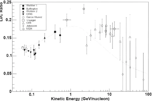
3.6 _{Li/C ratio versus kinetic energy (GeV/nucleon). The solid curve is from the} GALPROP prediction assuming low solar modulation (potential D=500MV). See the table 3.1 for the corresponding reference... 42

3.7 7Li/6Li ratio versus kinetic energy (GeV/nucleon)... 42

4.1 The AMS-01 schmetic and sketch [1]... 44

4.2 _{AMS-01 magnet dimensions and field orientation [1]. 64 groups of Nd-Fe-B block} are arranged such that a uniform 0. 15T dipole field is created inside the bore, and less than 60 G outside to prevent interference with electronics... 44

4.3 An exploded view of AMS-01 tracker ladder... 45

4.4 The tw o upper TO F planes...47

4.5 AMS-01 in the space shuttle Discovery... ₅₀

4.6 Zenith angle of AMS-01 in ten-day flight, from [69]. The cartoon on the right illustrates the definition of zenith angle... 51

5.1 _{Rigidity resolution as a function of rigidity for Li, B and C... 57}

5.2 Scintillator paddle occupancy for each TOF plane... 58

5.3 Schematic view of residual distance calculation... 59

5.4 _{Mean energy loss for pions in liquid hydrogen, gaseous helium, Aluminum, iron,} tin and lead [4]... ₆₀

5.5 _{Occupancy level for ladder 9 on the second layer of Tracker. The red line} indicates the level of 65% of average occupancy in that ladder... 61

5.6 _{Average energy deposition on Tracker as a function of velocity from 0.6 to 0.95.} The function for solid curves is -_dx = A -

p--",

5.7 _{Mean energy deposition on Tracker for Charge from 3 to 8. Red curve is the fit to} six Gaussians. Nitrogen and Oxygen are suppressed due to the ACC triggering by 6 ray s... _{. . .. 6 3} 5.8 _{The longitude and latitude coverage of AMS-01 flight. (a) is in the Geographic} Coordinate system and (b) is in the Geomagnetic Coordinate system. The South Atlantic Anomaly (SAA) is labeled. The discontinuities are due to the trigger suppression of proton data... ₆₅

5.9 _{AMS-01 proton spectra at different geomagnetic latitudes. The apices in the low}

proton s 66...-... 6 6

5.10 (a) Full trace-back track of the proton from the birth in the atmosphere (10 s) to the

detection by AMS-01 (0 s). The altitude is measured from the Earth's center.

(b) shows its partial track, which demonstrates the three motions in the Earth's

magnetic field: cyclotron, bounce and drift... 67

5.11 Proton spectrum at geomagnetic latitude less than 0.1. Red curve represents the

proton spectrum after removing the Albedo and Trapped protons... 68

5.12 (a) Lithium and (b) Carbon spectra. Black histogram is the AMS-01 data after

selection cuts discussed in section 5.1-5.4. Blue and green histograms are the

identified atmospheric events after back tracing... 69

5.13 Spectra after selection cuts of (a) Lithium and (b) Carbon. 8349 Lithium and 22709 Carbon events are kept after selection cuts... 70

5.14 Acceptance for Lithium and Carbon. Efficiency correction has been included... 72 5.15 Resolution Matrices for (a) Lithium and (b) Carbon. The darkness represents the

probability. Notice that Lithium has better rigidity resolution than Carbon.

Squares are due to calculation coarseness in domains... 74

5.16 Unfolded (a) Lithium and (b) Carbon spectra, compared with folded spectra.

Notice that Carbon spectrum has larger correction due to the worse rigidity

resolution ... . 75

6.1 Lithium to carbon ratio measured by AMS-01. Errors include statistical errors of data, and a 3.5% detector efficiency (see section 5.6.2), summed in quadrature since they are uncorrelated. The solid curve is the best fit from GALPROP including solar modulation (CD=580MV for AMS-01 flight), see section 6.3. The other six experiment data sets were converted from kinematic energy to rigidity for comparison, refer to table 3.1 for the corresponding references. The reason these measured values lie below the prediction curve is that the solar activity was much

smaller when these measurements were carried out than during the AMS-0 1 flight in 19 9 8 ... . . 7 8

6.2 Lithium Mass distribution fit assuming 7Li/6Li= 12.1. The black dots are the

AMS-01 lithium data, two shadowed histograms represent the Monte Carlo 6Li

(brown) and 7Li (blue), and the red histogram is the sum of Monte Carlo 6Li and 7Li

as the best fit to the data... 80

6.3 Lithium Mass distribution fit. Normalization factors for Monte Carlo 7Li and 6Li

are both free param eters... 81 6.4 Confidence intervals for the Monte Carlo 6Li and 7Li normalization factors. The

two normalization factors are negatively correlated. The correlation has been

6.5 7_Li/6_{Li ratio versus rigidity. The previous experimental data have been converted}

from the kinetic energy to rigidity, refer to table 3.1 for the corresponding references. Because of the conversion, the results have upward trend compared to Figure 3.7. The blue curve is from the GALPROP prediction... 83

6.6 _{Confidence intervals for diffusion coefficient Dxx and Alfven velocity VA. The}

color code represents the value of Chi Square x2. Inner contour is for 50%

confidence level and the outer one is for 68.3% (1) confidence level... 85

6.7 _{Projected ratio measurements [72]: (a) B/C results from 6 months of AMS-02 and} (b) 10Be/9Be results from 1 year of AMS-02... 87 A. 1 Schematic view of one cycle of shock wave acceleration...92

List of Tables

2.1 Li/H abundance ratio measurements. Refer to section 2.2 for details of the MPH stars and CMB measurements... 23 2.2 7Li/6_{Li isotope ratio measurements... 24}

3.1 Summary list of previous experiments which measured cosmic ray lithium isotopes with energy < 1TeV/nucleon... 41 5.1 Selection cuts on Lithium and Carbon data... 71

Chapter 1

Introduction

In June of 1998 the Alpha Magnetic Spectrometer (AMS-01) [1, 2] launched on the Space Shuttle Discovery for a 10 day mission at an altitude between 320 and 390km, a suitable place for cosmic ray measurement because of the absence of atmosphere. The AMS experiment is designed primarily to search for dark matter and antimatter by studying cosmic rays. During the flight, 100 million events with kinetic energies at MeV to TeV scales were collected and precisely measured. This thesis presents the results of cosmic ray lithium to carbon ratio and lithium isotope ratio using the AMS-0 1 data.

For more than thirty years lithium isotopes (6Li and 7Li) have been recognized as an efficient probe of nueclosynthesis in the universe [3]. The primordial lithium isotopes produced in the Big Bang Nucleosynthesis (BBN) retain the footprint of the early universe and provide tight constraints on cosmological constants [4, 5]. The lithium isotopes in cosmic rays, stellar atmospheres, and the interstellar medium record subsequent stages of evolution [3, 6, 7, 8]. Even with the large number of observations at different astrophysical regions, there are still many unsolved questions on lithium isotopes: the reason for large discrepancy of 7Li/6_{Li ratio between solar system and cosmic rays is not yet clear [9, 10], and}

the recent two "Lithium Problems" [11, 12] for primordial lithium isotopes have spurred many new hypotheses on stellar models, BBN and cosmological/galactic cosmic rays. The precise experimental characterization of cosmic ray lithium isotopes is essential for solving these problems.

The cosmic ray lithium to carbon ratio, so-called 'secondary to primary' ratio, has long been used to probe models of cosmic ray propagation within the Milky Way, because most cosmic ray lithium isotopes are expected to be produced by the spallation of carbon, nitrogen and oxygen during their propagation through the galaxy. GALPROP [6], a diffusive galactic propagation model, has been widely used by many cosmic ray experiments, such as AMS,

PAMELA, Fermi/GLAST, etc. to interpret their observations. The cosmic ray lithium to carbon ratio can provide good constrains on the propagation parameters in GALPROP, and

thus further assist in the interpretation of these many experiments' results.

Since 1970's, the direct measurement of cosmic ray lithium isotopes, especially the Li/C and 7 _Li/6

Li ratios, has been achieved through both balloon-borne and space-bome experiments. _{But most measurements are done in the energy region below 1 GeV/nucleon.} Only a very small amount of data is available above 1 GeV/nucleon with low statistics and energy resolutions.

From the AMS-01 data, about 4 thousand lithium and 20 thousand carbon nuclei have been identified using the combined information of the silicon tracker and the scintillators, which allows us to measure the Li/C and 7_Li/6_{Li ratio in the high energy region with an}

unprecedented level of statistics. The Li/C ratio versus rigidity, defined as momentum over charge, can then be used to constrain two critical Galaxy propagation parameters, the diffusion coefficient D xx and the Alfven velocity _VA.

The outline of the thesis is as follows,

Chapter 2: Mysteries of Cosmic Lithium describes the origin and production mechanism of

lithium isotopes, and briefly reviews the "Lithium Problems" and proposed model explanations.

Chapter 3: Charged Cosmic Rays presents a general overview of characteristics of cosmic

rays: their origin, acceleration and propagation in the Galaxy. Previous results for other cosmic ray lithium isotope experiments are summarized.

Chapter 4: The AMS-01 describes the details of the experiment, mission, design, flight, and

constructions of sub-detector components relevant to the data analysis in the following chapter.

Chapter 5: Data Analysis lays out the specific analysis techniques used to obtain the lithium

and carbon events from the AMS-0 1 raw data.

Chapter 6: Results presents the final results of the Li/C and 7_Li/6_{Li ratio and the best fit to}

the propagation parameters in GALPROP.

Chapter 2

Mysteries of Cosmic Lithium

The abundance of lithium isotopes (6Li and 7_{Li) provides important information about the}

early universe, galactic evolution, stellar formation and cosmic ray propagation and interactions [3]. Unlike other heavy (Z>2) nuclei, which are synthesized in stellar formation, lithium isotopes are fragile and can be easily destroyed in the hot star centers. They are produced in many other ways, such Big Bang Nucleosynthesis (BBN), cosmic ray nuclear

reactions, and non-equilibrium stellar processes such as supernova or giant star explosions. The specific mechanisms of stellar production are still under debate.

Recently, two so-called "Lithium Problems" have arisen regarding the disagreement of the primordial lithium abundance between the experimental observations and the predictions of the standard BBN model. Many speculative resolutions have been proposed, but the actual resolution of the Lithium Problems is still far from clear.

Cosmic ray lithium isotopes play an important role in attempts to resolve the above problems.

In this chapter, we introduce present knowledge of the origins and the production mechanisms of lithium isotopes. The "Lithium Problems" and possible solutions are briefly reviewed.

2.1 Origin of Lithium Isotopes

The stellar formation of chemical elements was first proposed by Fred Hoyle and his collaborators in 1957 [13]. While this idea proved to be correct for heavy nuclei, from carbon to uranium, it encountered big difficulties when trying to account for the abundances of light elements such lithium, beryllium and boron (LiBeB), which are very fragile and

rapidly consumed by radiative capture reactions in the stellar center.

Lithium has two stable isotopes, Lithium 6 (6_{Li) and Lithium 7 (7Li).}

Since they have low binding energies, 5.3MeV/nucleon for 6Li and 5.6 MeV/nucleon for 7Li, they are both destroyed in stellar interiors via 6 _Li(p,3_He)4_{He at ~2 million K and} 7_Li(p,a)4_{He at ~2.5 million} K respectively. _{Significant abundances of lithium can only be produced in regions of rapid} expansion and cooling, e.g., the Big Bang or explosive nucleosynthesis, or in cool rarefied matter such as the interstellar medium (ISM).

2.1.1 Big Bang Nucleosynthesis (BBN)

Li can be traced back to the very beginning of the universe, at the end of the

"First Three Minutes" after the Big Bang, when the BBN started [14]. At that time the temperature dropped to 109_{K which allowed the neutrons and protons to start to form} deuterons. _{In sequence, more reactions took place for roughly 20 minutes until the} temperature and density of the universe fell below what is required for nuclear fusion. The nuclear reactions of BBN are illustrated in the Figure 2.1. The specific reactions involved in the production and destruction of Li are emphasized by the red rectangle.

7 Be 12 11. 1_{H < n} H F y 11 2. 'H +n _{2 2H +,y} 3He P- He 13 7i3. 2H + 'H + He + y 4. 2H +2H - He +n 5. 2_{H +}2_H

₊

n

Figure 2.1: The nuclides involved in Big Bang Nucleosynthesis and the most important reactions that relate them. *The beta decay of 7_{Be occurs late in the time of recombination}

BBN hypothesis has been a reliable probe of the early universe, and depends on only one free parameter: baryon density or baryon to photon ratio (9) [4, 15]. The concordance between theory and observation of the abundance of the light elements 2H, 3He, 4He and 7Li

provides a powerful tool for obtaining the baryon to photon density and a consistency check for the model itself. Figure 2.2 shows the abundance of the light elements as a function of 1

[4].

7Li produced in BBN, so-called "primordial" 7Li, has abundance of 7Li/H

-10

complicated shape of the abundance curve results from two competing processes, reaction 9 and 10. At high rj, the bulk of 7Li is produced as 7Be, which will be converted to 7Li after BBN. The sum of these two processes results in the shape of abundance curve.

Deuterium abundance is always taken as the best "baryometer" to constrain the value of

,i, because it is highly sensitive to i and has no other astrophysical source. For comparison,

primordial 7Li abundance was also measured with old halo stars and globular clusters. This

direct measurement is in significant disagreement with a 7Li abundance derived from measurements of the Cosmic Microwave Background (CMB) radiation shown in Figure 2.2. The details will be discussed in the later section as one of the two famous "Lithium Problems".

In addition to the light elements listed in Figure 1.1, trace amount of 6Li, Be and B are also produced in the BBN. 6Li abundance is estimated to be of 6Li/H~10-14 _{[8]. The}

nuclear reactions for the production and destruction are:

4_He+ 2_{H -} 6_Li+y

6 Li + 'H4He +3He

2.1.2 Galactic Cosmic Ray Production

The Lithium abundance in the solar system and galactic disk has been measured to be Li/H~1-2x10-9 [8, 16, 17], which appears enriched by factor of 10 since BBN. Therefore

there must be other mechanisms which generate the major part of lithium isotopes during the galactic evolution, such as cosmic ray nuclear reaction.

The idea of Galactic Cosmic Ray (GCR) production of lithium, as well as beryllium and boron, was introduced in 1970 by Reeves [18], who conjectured that the light elements were made by the interaction of fast GCRs with the interstellar medium. The enrichment of light elements can be illustrated by the comparison of the element abundance in cosmic rays and the solar system as shown in Figure 2.3. Lithium abundance in cosmic rays is 4 orders of magnitude larger than the solar system abundances, proving GCR production to be an

0.27 0.26 0.25 0.24 0.23 10-3 10-9 5 7Li/H Ip 10-10

0.005 Baryon 0.01density UBh2 0.02

1 3 4 5 6

Baryon-to-photon ratio q x 1010

0.03

7 8 9 10

Figure 2.2: The primary abundances of 4_He, 2_H, 3_{He, and} 7_{Li as predicted by the standard}

model of BBN [4]. The bands show the 95% CL range. Boxes indicate the observed light element abundances (smaller boxes: +2G statistical errors; larger boxes: +2G statistical and systematic errors). The narrow vertical band indicates the CMB measure of the cosmic baryon density, while the wider band indicates the BBN concordance range (both at 95% CL). The 5-year WMAP study [19] reports -1 = 6.23 + 0.17 x 10-10, see section 2.2.

10 i 10 10 10I () 10 10 10 s 10 -6 10 10 ₂₅ Charge Z

Figure 2.3: The relative chemical abundances for GCRs (solid line) and within the solar system (dashed line) [20]. The differences between these two regimes are most evident for the secondary particles (LiBeB) and the sub-Iron group.

0.01 I % I I

0 100 200 30D 400 500 600 700 Ekin (MeV)

p+N -+LI

.1 1 ID 01 1 10

Ekin, GeVinuceon Ekin, GeV/nucleon

(b)

Figure 2.4: Lithium production cross section measurements: (a) a fusion [21]. The lines are simple exponential fits. (b) Spallation of CNO [22]. Solid circle symbols are

accumulated data and dashed lines are evaluated cross sections in [22].

C' 0

Fe

V) +

La B Sc

Lithium isotopes are generated by two GCR production processes: spallation of carbon, nitrogen and oxygen (CNO) and a fusion [1, 21]. Spallation occurs when energetic cosmic

CNO nuclei interact with interstellar protons and a particles (or vise versa) and split into light

elements. Most cosmic ray LiBeB, so-called secondary particles, are produced in this way. The secondary to primary abundance ratio plays an important role for cosmic ray propagation in the galaxy which will be discussed in next chapter.

The a fusion produces only 6Li and 7Li, through reactions 4He + He 4 6Li _ 2H and 4He

+ 4He 4 7Li + H. It plays a major role in production of _{6Li and} 7_{Li in the early galaxy when} the interstellar medium contains very little CNO. But a fusion does not contribute much to the present cosmic rays above 600 MeV, because the production cross section falls rapidly, essentially exponentially, with the increasing energy [21]. The production cross sections for both processes are shown in Figure 2.4.

The 6Li abundance in the solar system and ISM is 6_{Li/H~10* [20], which is by four} orders of magnitude larger than the BBN production. Therefore GCR production of 6

Li

accounts for almost the entirety of the 6_{Li in the universe.}

2.1.3 Stellar Production

Problems arose when comparing the GCR lithium isotope ratio to the ratios in solar system and galactic gas composition. As we can see form Figure 2.4, GCR produces almost equal amount of 6_{Li and} 7

Li, a result that has been observed by many cosmic ray experiments [23, 24]. _{But the measurements on protosolar meteorites [25, 26], Earth [27] and the present ISM}

[28] yield a value for 7

Li/6_{Li ratio -12, indicating that this ratio has remained nearly constant} during the last 4.5-5 Gyr. Therefore, there must be some extra sources able to produce large amounts of 7Li without generating 6_Li.

The Asymptotic Giant Branch (AGB) star 7_{Li production has been studied intensively}

since 1970's [29]. The AGB stars are post 4He-core burning objects with a C-O core, around which a H-burning shell operates, and a deep outer convective envelope. The 3_He(a,y)7_Be

reaction takes place in the deep interior of a star and then 7Be is transported via the convection zone to outer regions where the temperature is much cooler. The reaction

7_Be(e~,v)7_{Li can then produce} 7

Li under conditions where the lithium is not rapidly destroyed.

This beryllium transport mechanism was first suggested by Cameron in 1955 [30]. Now more and more lithium-rich stars have been experimentally discovered [7, 9]. However, it is hard to estimate their total contribution since it depends on the estimated number of such stars, which are hidden from observation by their own wind [9]. The estimated contribution is roughly 10-50% of total 7_{Li in the universe.}

Another major 7Li production mechanism is the neutrino nucleosynthesis in Type II supernovae (SNII) [31, 32]. When the core of a massive star collapses into a neutron star, the flux of neutrinos is so great that despite the small cross section they may still induce considerable nucleosynthesis. The neutrino process in the helium shell is responsible for the most of the 7Li production in SNII through the following reactions.

v + 4_{He 4} 3_{He +v'+n} 3_{He +} 4_{He 7+} 7_Be

7Be + e-

+

Eventually, 7Li is injected into the ISM by the Supernova explosions. Like the AGB star case, there are also large uncertainties on the total yields of the SNII [10]. Other stellar mechanisms, such as explosive hydrogen burning in nova explosions, may also contribute to the 7Li enrichment [33].

In conclusion, while 6Li only has one simple source, GCR production, 7Li owes its abundance to three different mechanisms: BBN, GCR spallation and fusion, and stellar nucleosynthesis. None of the stellar mechanisms has been quantitatively and accurately estimated nor strongly constrained by observations.

Observations of lithium isotope abundance at different astrophysical local sites are listed in tables 2.1 and 2.2.

Sample Li/H ratio Method Reference

High energy ~10-4 Direct cosmic ray 4

cosmic rays nuclei measurement

Population I Stars 1-3x10_9 _{Li I X=670.7nm}

[16, 34]

and interstellar gas Doublet

Super Li-Rich stars 10-_107 Li I X=670.7nm _{[9, 35]}

(7Li only) Doublet

Metal-poor halo 1.23x10~10 _{Li I X=670.7nm}

[11, 36]

(MPH) stars (6Li) -6.3x10-1 2 _doublet

WMAP+BBN ('Li) 5.24x10~"' CMB measurement [4, 19]

(6Li) ~ 10-"

Table 2.1: Li/H abundance ratio measurements. Refer to section 2.2 for details of the MPH stars and CMB measurements.

Sample 7_Li/6_{Li ratio Method Reference}

Cosmic rays 093 _{Direct cosmic ray [24]}

(1GeV/n) _{nuclei measurement}

Earth -12.1 Mass spectrometer [27]

Meteorites (pre-solar) -12.5 Mass spectrometer [25]

ISM (present) -12.5 Li IX670.7nm [28]

doublet

MPH stars -20 Li I X670.7nm [11]

doublet

Table 2.2: 7_Li/6_{Li isotope ratio measurements.}

2.2

Lithium Problems

The lithium problems arise from the significant discrepancy between the primordial 7_{Li and} 6Li abundance as inferred from the observations of metal-poor halo (MPH) stars and predicted by BBN theory and the Wilkinson Microwave Anisotropy Probe (WMAP) [37] baryon

density.

The first lithium problem: the latest WMAP-based analysis [11] predicts a primordial 7Li abundance of 7_{Li/H=5.24i07 x 10-10, which is by factor of 4.3 larger than the MPH}

stellar observations of Li/H=1.23to+.3 x 10-10 [36]

The observation of primordial Li was promoted first by Spite and Spite in 1982 [3], who showed that lithium abundance (>95% is 7_{Li) in the MPH (Population II) stars was}

independent of metallicity for [Fe/H]<-1.5*. The constant lithium abundance, commonly called "the Spite plateau", was interpreted as resulting from a pre-galactic origin, from BBN. In subsequent years, a voluminous literature has accumulated on the lithium abundance in MPH stars, but the published lithium abundance varied little from the initial plateau measurements [11, 38, 39]. In 2000, Ryan reported a slight dependence of lithium abundance on the metallicity in MPH stars [36], which was attributed to enrichment of galactic cosmic ray lithium. The primordial lithium abundance is then identified with the extrapolation of the observed lithium abundance to zero metallicity, commonly cited as Li/H= 1. 230.34x 10-10. This value is recently confirmed by Ultraviolet and Visual Echelle Spectrograph (UVES) on VLT telescopes [11], which has the highest spectral resolution of any telescope for this wavelength.

This simple but beautiful picture has been shaken by recent observations from WMAP.

By precisely measuring the CMB anisotropies and mapping these anisotropies to the "acoustic"

baryon density, as the only free parameter for BBN, to unprecedented accuracy to be

fiBh2 = 0.02273 + 0.00062 or equivalent to baryon to photon density 11 = 6.23 + 0.17 x

10-10 [40]. Adopting this baryon density in the standard BBN model, Figure 2.2 shows the

predicted abundance of 4He, 2H, 3He, and 7Li. The primordial 7Li abundance is expected to

be 4.3 times larger than the plateau value. Additional support for the reliability of baryon density comes from the excellent agreement of 2H abundance achieved from the WMAP

prediction and the measured value from quasar absorption systems [41]. This perfect agreement makes the discrepancy between WMAP predictions and measured values of lithium abundance even harder to explain.

The second lithium problem is even more serious: a 6Li plateau of 6Li/H~6.3 X 10-4

has been found [42, 43] and recently confirmed by UVES/VLT, on the MPH stars which favors the primordial origin, but Standard BBN should only produce trace amounts of 6Li, with an abundance of 6Li/H ~10-14; a two orders of magnitude discrepancy.

The 7_{Li and} 6_{Li plateaus measured by UVES/VLT are shown in Figure 2.5.}

2.3

Proposed Model Explanations

Many mechanisms have been invoked to explain these two lithium isotope problems.

For 7Li, systematic errors on lithium spectra measurements and nuclear reaction rate models cannot account for such a significant discrepancy [19], and discarding WMAP estimation of baryon density will introduce more problems. Therefore the depletion of 7Li during stellar evolution seems presently the most favored solution. 7Li are assumed to be destroyed by Li(pa)4He when transported deep into the stellar center due to atomic diffusion or rotationally-induced mixing. Many so-called non-standard stellar models have been developed by including the rotation, diffusion and mass loss effect to reconcile the 7Li reduction [44, 45]. But the depletion has only been observed on the main sequence stars, and may fail on the requirement to deplete 7Li in different stars of different surface temperature, mass and rotation velocity without introducing large dispersion in the plateau.

Since 6Li are assumed to be only produced in the cosmic rays, the excessive Li abundance found on MPH stars has been mostly attributed to cosmological/galactic cosmic rays. The pre-galactic large-scale structure formation [46] or the explosion of Population III stars [47] produced cosmological cosmic rays which consisted of mostly protons and a particles. As we discussed in section 2.1.2, 6Li and 7Li were then produced by cosmic ray a fusion and brought to the atmosphere of MPH stars. Galactic cosmic rays are also expected

to provide extra 6_{Li and} 7_{Li by CNO spallation to MPH stars [48].}

To reconcile the potential depletion of both lithium isotopes during the stellar evolution, the production of 6Li by the interaction of in situ solar-like flares [49] with MPH stellar

atmosphere is also proposed as one explanation.

0 3.0 2.5 2.0 1.5 1.0 0.5 0.0 -3.0 -2.5 -2.0 -1.5 [Fe/H] -1.0 -0.5 0.0

Figure 2.5: Observed logarithmic abundances of 7_{Li (open triangles) and} 6_{Li (filled circles)}

as a function of [Fe/ H] for UVES. The large circle corresponds to the solar system meteoritic 6Li abundance [43], while the solid line is the predicted 7Li abundance from WMAP+BBN prediction [19]. The dotted line is zero metallicity 7_{Li abundance [36] and}

dashed line is the average 6_{Li abundance for UVES. loge(Li) is defined as logE(Li)}

=

log(Li/H) + 12.

A mechanism that can solve the two lithium problems simultaneously has been proposed by incorporating non-standard model particles, such as the neutralino or gravitino [12]. The

decay or annihilation of these particles (as relics of the very early universe) will inject thermal neutrons into BBN. Neutrons will reduce the primordial 7_{Li by destroying the} 7_{Be which is}

WMAP+BBN

Li

6

_Li

-expected to be converted to 7Li after BBN. Thermal neutrons will also develope a nuclear

cascade to produce more Deuterium which results in excessive 6Li production. But the existence of such particles is not yet experimentally proven.

Nevertheless, cosmic ray lithium isotopes may play an important role for the excessive

6Li abundance on MPH stars. To solve the 6Li plateau problem, both a better understanding of cosmic rays and a more accurate measurement of cosmic ray lithium isotopes are

necessary.

* In astrophysics, metallicity is defined as the proportion of matter made up of chemical elements other than hydrogen and helium. It is usually expressed by [Fe/H] = logo10

(Ne)

(

-)

NH sun

atoms per unit of volume respectively. The metallicity provides an indication of age since older stars have lower metallicities than younger one, e.g. Sun is one of the metal-rich Population I stars.

Chapter 3

Charged Cosmic Rays

Nearly 100% of the galaxy's 6Li and 10-20% of the 7Li is conjectured to be produced through

cosmic ray spallation and fusion during galactic propagation. The direct measurement of cosmic ray lithium isotopes therefore provides an essential probe of the nature of

characteristics of these propagation processes.

A general overview of the features of cosmic rays, including their origin and acceleration,

will be given in the first part of this chapter. Then we will focus on the details of the galactic propagation of cosmic rays. The propagation of cosmic rays through the local solar

environment and the Earth's magnetic field will also be discussed. Finally, we will discuss previous cosmic lithium ratio experiments and summarize their results.

3.1

Cosmic Ray Sources and Acceleration

Cosmic rays are energetic charged particles reaching the Earth's atmosphere from all directions. The discovery of cosmic rays came in 1912 with the first pioneering balloon measurements of an increasing ionization rate with altitude [50]. Since then, cosmic ray composition and intensity have been measured by many satellites, balloons, and ground-based experiments.

Cosmic ray energies span more than 20 orders of magnitude, from several eV to 102 eV and above, and the rough composition of cosmic rays is 86% protons, 11% ionized helium, 2% electrons and positrons, and trace amounts of heavier elements [4]. Hydrogen and helium are produced in the Big Bang Nucleosynthesis (BBN) and heavier elements from carbon to nickel are synthesized in the stellar evolution by the nuclear fusion. The elements above iron are typically produced in supernova (SN) explosions. The nuclei generated before propagation are called primary cosmic rays. Secondary cosmic rays, such as lithium, beryllium and boron (LiBeB), are generated by spallation of primary nuclei in the interstellar medium during propagation. Therefore, the LiBeB nuclei provide important information of

Galaxy chemical evolution and cosmic ray propagation [3, 6]. The major components of the primary cosmic ray nuclei are given in Figure 3.1.

10

Sx0

1i

1

1 11al

' ' '"'nal

1n

Kinetic energy per particle (nucleus) [GeV]

Figure 3.1: _{Major components of the primary cosmic radiation from [4].}

In the intermediate energy range from 0.1 GeV to 106 GeV, the cosmic ray flux can be described by a single power law distribution [2],

nucleons IN (E) ~ 1.8 x 10 4_{E -Y muces}

(3.1)

m 2 sec sr GeV

The spectra index y is 2.7 for over all flux and takes value from 2.5 to 3 for individual species. The cosmic rays in this energy range are believed to be produced primarily within the galaxy. A strong support to this local source hypothesis comes from the observed power-law spectrum for high energy electrons. _{Inverse-compton scattering with the Cosmic Microwave} Background (CMB) would destroy this spectrum, if they were produced at distances greater than 300 kpc [51].

assumed that the charged particles were randomly scattered by the moving magnetized clouds, which resulted in net energy gain per bounce proportional to the square of the velocity of the magnetized clouds. That is why the mechanism is called Second Order Fermi Acceleration. Although such a process can explain the power-law spectrum, it is unable to accelerate particles to GeV energy.

The First Order Fermi Acceleration in Supernova Remnant (SNR) shock wave is now a widely accepted mechanism for the efficient acceleration of cosmic ray particles to energies

up to 106 GeV [53]. The model has been supported by recent observations of X-ray and gamma ray emissions near SNs, which has revealed the presence of energetic electrons accelerated in the SN shock waves. Assuming a galactic rate of 3 supernovae per century and an explosion energy of 10 erg, less than 10% of the energy is needed to channel into acceleration to sustain the average cosmic ray energy density, estimated to be ~1eV/cm 3.

The details of the first-order and second-order Fermi acceleration mechanisms will be discussed in the Appendix A. In summary, each time the particle up-scatters off the SNR shock front, it gains energy proportional to the velocity of the shock wave. Higher and higher energies are achieved when the particle repeatedly crosses and re-crosses the shock front. Meanwhile, the particles' probability of escaping the SN magnetic field altogether increases with velocity. The combination of these two effects would result in a power law spectrum with index ~ -2.1 [54]. The observed much steeper cosmic ray spectral index of

-2.7 can be achieved by accounting for the energy dependence of the probability of a cosmic ray particle to escape to infinity during galactic propagation.

The upper limit for the accelerated energy comes from the increasing gyroradii of the charged particles compared to the size of the shock wave. The steepening at 106 GeV in the cosmic ray spectrum, usually called the Knee, is believed to represent the maximum energy transferable from the SNR shock waves. The spectrum above the Knee flattens again at the

109 Gev, the so-called Ankle [55]. The particles observed at this energy have gyroradii of the order of the galaxy's size. Therefore they are still speculated to be of the galactic origin and accelerated at the termination of galactic wind [56]. The particles with energy above

1010 GeV are called Ultra High Energy Cosmic Rays (UHECRs). Their origin and

acceleration mechanism are still debated. The gyroradii indicate extragalactic source, i.e. Gamma Ray Burst (GRB) [57]. But the extragalactic UHECRs should have been highly suppressed by the "GZK-cutoff' [58] due to the energy losses of protons by photon-pion-production with the Cosmic Microwave Background.

Cosmic rays with energy below 1GeV/n are mostly from the solar wind as discussed later in section 3.3.

3.2

Galactic Cosmic Ray Propagation

Once accelerated by supernova shocks, cosmic rays spend ~107 years diffusing through the galaxy, confined by magnetic fields. During this propagation, cosmic rays spiral around magnetic field lines, frequently scattered by magnetic irregularities and turbulence. This process has long been interpreted as slow diffusion [54], which results in an isotropic distribution of charged cosmic rays as observed at Earth.

PPP_

halo

CRS

15 kpc 8.5 kpc

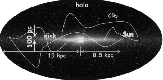
Figure 3.2: Side view of the Milky Way and schematic propagation of cosmic rays.

3.2.1 Galactic Structure

A cartoon representation of our galaxy and the propagation of cosmic rays is shown in Figure 3.2. The Milk Way has a form of a flat disk with a radius of -15 kpc (1 kpc= 3.086x 102 1_{cm) and a thickness of approximately 100 pc. The luminous matter of the galaxy is}

mainly distributed in the center bulge and the spiral arms on the disk. The galactic disk is surrounded by a spheroid halo of old stars and globular clusters, of which 90% lie within 30 kpc. The solar system lies at a distance of 8.5 kpc away from the galactic center. The cosmic rays will be confined inside the halo for ~107 years depending on their energies [59].

While traveling through the galaxy, cosmic rays interact with the Interstellar Medium

(ISM), which consists of clouds of gas and dust, magnetic fields both coherent and turbulent,

radiation fields from starlight, and CMB radiation. Interaction processes include energy loss through ionization, synchrotron radiation and inverse-Compton scattering; energy gain by the

stochastic acceleration; and nuclear reactions such as radioactive decay and fragmentation. The interstellar gas and dusts have important effects for the secondary production. The

gas consists mostly of hydrogen in the form of atomic neutral hydrogen (HI) and molecular hydrogen (H2), and small portion (about 10%) of Helium. The average density of interstellar

matter is estimated to be 1 nucleon/cm3 [60], from various measurements [61, 62, 63].

The average magnetic field in the Galaxy is on the order of 10-6 Gauss. Magnetic turbulence and irregularities play important roles to confine and reaccelerate the energetic particles.

The Interstellar Radiation Field (ISRF) includes photons emitted from stars and CMB radiation. The latter is well-known by its black body spectrum.

3.2.2

Propagation Models

Two general classes of models have been proposed to describe the propagation of cosmic rays in the galaxy: the Leaky Box Model (LBM) and the Diffusion Halo Model (DHM). The LBM uses the simple picture of an equilibrium system, in which the cosmic ray sources, interstellar gas, and radiation field are uniformly distributed in a confinement volume (the galaxy), and these sources are constant in time [54, 64]. The diffusion is approximated by the mean escape time (-esc), the mean time spent by a cosmic ray in the containment volume. The recent modified LBMs are quite compatible with data [64, 65, 66], but the escape mechanism and the physical size of the volume are still not well addressed [67].

The DHM model accounts for the actual structure of the galaxy, cosmic ray source distributions, and interactions of cosmic rays with the interstellar medium, which are all incorporated into the transportation equation [6],

adt U4, p. t 0 2 a10

=q(i,p,t)

V(DxVxi$-Y$)

-(V1 - -A$- A$ (3.5)

ap 3 Tr Tr

Note that in [6]

. $(r, p, t) is the density per unit of total particle momentum at position r with $p(p)dp = 4Trp2f() in terms of the phase-space density f().

. q(r, p, t) is the source term including the primary sources and contributions from spallation and decay.

. DXX is the spatial diffusion coefficient.

. V is the convection velocity. Since there is no direct observational support for the convection, we will not use this term in the later analysis.

p

= _{is the momentum gain/loss rate.}

. Tf is the timescale for fragmentation.

* Tr is the timescale for radioactive decay.

A variety of analytical and numerical approaches to the transportation equation can be

found in the literature [68]. GALPROP [6] is a widely used numerical simulation code developed by Igor Moskalenko and Andrew Strong. It has been applied towards indirect Dark Matter signature searches in AMS-01 [69], PAMELA [70] and FERMI/GLAST [71], and will also be used for AMS-02 experiment [72]. Understanding of this program becomes important interpreting future cosmic ray data.

3.2.3 GALPROP Properties

The GALPROP model is three-dimensional, with cylindrical symmetry in the Galaxy; the basic coordinates are R (Galactocentric radius), z (distance from the galactic plane) and p (particle total momentum). The propagation region is bounded by a cylinder with Rh=30 kpc and Zh=1-20 kpc, with free escape assumed. The input source is the primary cosmic rays

after the SNR acceleration. Once the input source distribution and the boundary condition are determined, GALPROP solves the time-dependent equation 3.5 for all species by advancing the solution in time until a steady state is achieved.

There are three basic parameters which govern the GALPROP model: halo size Zh,

diffusion coefficient Dxx, and Alfven velocity VA. The halo size determines how long the

cosmic rays will be contained in the galaxy, and the diffusion coefficient and Alfven velocity characterize the essential diffusive reacceleration process in the propagation.

Halo height Zh and the radioactive clocks

Long-lived unstable secondaries are good probes of confinement of cosmic rays in the galaxy. Several of the best of these so-called radioactive clocks are 10_Be, 14_C, 26_{Al and} 54_Mn.

Among these nuclei, 10_{Be is the best measured and longest lived, with a half life of 1.5 million} years, comparable to the confinement time. The data on energy dependence of '0_Be/9_Be abundance ratio and the prediction from different propagation models are shown in Figure

3.3.

9Be (stable) and '0_{Be (unstable) are both secondaries and produced with similar cross section.}

In the low energy range with negligible relativistic time-dilation, 10Be is much depleted (in relation to 9Be) due to beta decay. Therefore, the larger the halo size, the less '0_{Be will be} observed. The best fit suggests the halo height of 4 kpc [6].

0 .6

# # i i

I I I I 1 l

0.5

1-2

0.3

0.2

_T

0.01

0.1

1

10

E

[GeV

nucleon']

Figure 3.3: Beryllium isotope ratio measurements from [24]. The listed experiments will be discussed in section 3.5. The solid line is the GALPROP model and the dashed lines are two Leaky Box Models [59].

Diffusion and Reacceleration

The concept of cosmic ray diffusion explains why energetic particles are "mixed" efficiently and are retained rather well within the galaxy. In the GALPROP model, diffusion terms include the spatial diffusion and momentum space diffusion through reacceleration. On the microscopic level, both diffusion types are the result of scattering on random moving magnetic fields, Alfven waves [73]. Alfven waves are transverse magnetic tension waves which propagate along magnetic field lines and can be excited in magnetized plasma in response to perturbations. The velocity with which Alfven waves propagate along the

1

magnetic field is called Alfven velocity VA. It is estimated to be VA = B/(4Trp-), where B is the magnetic field strength and p is the interstellar medium density.

The wave-particle scattering is of a resonant character so that a particle with Larmor radius r mainly interacts with waves which have a wave number of k = 1/r. Assuming a Kolmogorov spectrum for the MHD turbulence [6], the spatial diffusion coefficient has a power-law dependence on the rigidity and can be expressed as

1

D. = D0P(R/Ro)3 (3.6)

where Do is the diffusion constant to be determined, and R is the rigidity, Ro is the reference rigidity (see Appendix C).

A rough estimation of the value of the diffusion coefficient can be obtained by picturing

diffusion in a macroscopic level (in pc) [74]. Cosmic ray particles are scattered by the sudden change of magnetic field due to the presence of stars and other objects. In our neighborhood of the galaxy, the distribution of stars is roughly 1 per cubic parsec, therefore the mean free path of a charged particle X can be estimated about 3x 10'8_{cm. Supposing the}

particle has a velocity close to the speed of light, the propagation velocity is v = c/V, because it spirals along the magnetic field line. Then the diffusion coefficient can be calculated as D = v x A ~ 5 x 102 8 _cm2 _s-1.

This value is close to the one predicted by the GALPROP at 3GV (3 - 5 x 102 8 cm2 s-1) [6].

In addition to diffusion, charge particles are also accelerated by stochastically scattering off random MHD Alfven waves. To distinguish it from the primary acceleration in SNR shock waves, scattering off such Alfven waves is called reacceleration, which shares the same mechanism with second-order Fermi acceleration. In the transportation equation 3.5 the reacceleration is presented by diffusion in the momentum space and the diffusion coefficient is estimated as

p2V2

D pp = (3.7)

9DXX

where the Alfven velocity VA _{is the only free parameter. The ISM Alfven velocity is}

approximately 30 km/s [6, 73] and the exact value needs to be determined with the help of fitting the model to specific cosmic ray observations.

3.2.4 Li/C Ratio---Constraints on Dx and VA

Secondary particles are produced by the interaction of primary particles with the ISM during galactic propagation. Therefore, their spectra encode information about the propagation processes. The secondary to primary ratio, which cancels out the uncertainty on primary spectra, provides a good probe to the propagation parameters. The boron to carbon (B/C) ratio is often used because of its well-measured cross sections and abundant cosmic ray data.

The Li/C ratio is particular interesting since its production depends not only on the interaction of CNO, but also on tertiary interactions (Be-Li, B4Li), and therefore the Li/C ratio is more sensitive to variations between propagation models and provides further constrains on them. As we can see in Figure 3.4, the ratio (red curve) is featured by a characteristic peak at ~GeV/nucleon, which can be explained by the diffusive reacceleration process. _{In the low energy region, the reacceleration is strongest, which means that the} particles with higher energy have spent longer time in the galaxy and produced more secondaries. When energy becomes larger, diffusion dominates. Particles have more

chance to escape with higher energy, which results in less interaction of ISM and less secondary production. These two processes balance at the peak position.

The overall height of the Li/C ratio determines the diffusion coefficient, while the Alfven velocity determines the peak position, as illustrated in Figure 3.4.

0 0.22,- _{.2 .2~----.--- D =6.00 2}8 _om-s-t . . .. - ),,=5.75x 10 2 8 _{Cm s'} 0.18m 0.14 0.12-0.1 0.08 0.06[ 0.04 0.02F 0.1 1 10 100

Kinetic Energy (GeV/nucleon) (a) 0 0.22 A -. VA=20 km s -0.2 VA=3 6 km s' S0.18.. - ... VA=50 km s 0.16 0.12

0.1

Kinetic Energy (GeV/nucleon)

(b)

Figure 3.4: The effects of diffusion coefficient and Alfven velocity on the Li/C ratio, simulated by GALPROP. The red curve represents the theoretical Li/C ratio prediction from the default GALPROP parameter set Dx.=5.75cm2_{s~1 and VA=36kms-}1 _{[6, 75]. In (a) we fix} VA and change the Dxx, while in (b) we make opposite parameter adjustments.