HAL Id: hal-01664198
https://hal.archives-ouvertes.fr/hal-01664198
Submitted on 24 Apr 2018
HAL is a multi-disciplinary open access
archive for the deposit and dissemination of
sci-entific research documents, whether they are
pub-lished or not. The documents may come from
teaching and research institutions in France or
abroad, or from public or private research centers.
L’archive ouverte pluridisciplinaire HAL, est
destinée au dépôt et à la diffusion de documents
scientifiques de niveau recherche, publiés ou non,
émanant des établissements d’enseignement et de
recherche français ou étrangers, des laboratoires
publics ou privés.
inhibitory noise
Simona Olmi, David Angulo-Garcia, Alberto Imparato, Alessandro Torcini
To cite this version:
Simona Olmi, David Angulo-Garcia, Alberto Imparato, Alessandro Torcini. Exact firing time statistics
of neurons driven by discrete inhibitory noise. Scientific Reports, Nature Publishing Group, 2017, 7
(1), pp.1577. �10.1038/s41598-017-01658-8�. �hal-01664198�
Exact firing time statistics of
neurons driven by discrete
inhibitory noise
Simona Olmi
1,2,3, David Angulo-Garcia
2,4,5, Alberto Imparato
6& Alessandro Torcini
2,3,4,5,7 Neurons in the intact brain receive a continuous and irregular synaptic bombardment from excitatory and inhibitory pre- synaptic neurons, which determines the firing activity of the stimulated neuron. In order to investigate the influence of inhibitory stimulation on the firing time statistics, we consider Leaky Integrate-and-Fire neurons subject to inhibitory instantaneous post- synaptic potentials. In particular, we report exact results for the firing rate, the coefficient of variation and the spike train spectrum for various synaptic weight distributions. Our results are not limited to stimulations of infinitesimal amplitude, but they apply as well to finite amplitude post-synaptic potentials, thus being able to capture the effect of rare and large spikes. The developed methods are able to reproduce also the average firing properties of heterogeneous neuronal populations.Neurons in the neocortex in vivo are subject to a continuous synaptic bombardment reflecting the intense net-work activity1. In the so-called high-input regime, in which neurons receive hundreds of synaptic inputs during
each interspike interval2, the firing statistics of model neurons is usually obtained in the context of the diffusion
approximation (DA)3, 4.
Within such an approximation the post-synaptic potentials (PSPs) are assumed to have small amplitudes and high arrival rates, therefore the synaptic inputs can be treated as a continuous stochastic process characterized simply by its average and variance, while the shape of the distribution of the amplitudes of the PSPs is irrelevant5.
However several experimental studies have revealed that rare PSPs of large amplitude can have a fundamental impact in the network activity6, 7. Furthermore, the experimentally measured synaptic weight distributions
dis-play, both for excitatory and inhibitory PSPs, a long tail towards large amplitudes and a peak at low amplitudes6–12.
The effect of rare and large excitatory post-synaptic potentials (EPSPs) has been recently examined for generalized leaky integrate-and-fire (LIF) models with generic EPSP distributions13 and in balanced sparse networks for
con-ductance based LIF neurons with log-normal EPSP distributions14. The presence of few strong synapses induce
faster and more reliable responses of the network even for small inputs13, 14. Interestingly, in ref. 14 it has been
shown that a single neuron driven by random synaptic inputs log-normally distributed reveals a clear aperiodic stochastic resonance15, 16, which is not evident for Gaussian distributed EPSPs.
However, even for the simple case of LIF neurons exact analytic results are still lacking for large PSPs with generic synaptic weight distributions, apart for the case of the exponentially distributed PSPs reported in ref. 17. In particular, Richardson and Swarbrick have been able to obtain the statistics of interspike interval (ISI) for LIF neurons receiving balanced excitatory and inhibitory Poissonian spike trains with exponentally distributed syn-aptic weights17. Furthermore, results for generic EPSP distributions have been obtained in ref. 13 by developing a
semi-analytic approach to solve the continuity equation for the membrane potential distribution.
In this paper, we report exact analytic results for the firing time statistics of neurons receiving inhibitory Poissonian spike trains for various synaptic weights distributions. Namely, we estimate the firing time statis-tics for LIF neurons subject to inhibitory post-synaptic potentials (IPSPs) (with instananeous rise and decay 1Weierstrass Institute for Applied Analysis and Stochastics, Mohrenstraße 39, 10117, Berlin, Germany. 2Aix Marseille Univ, Inserm, INS, Institut de Neurosciences des Systèmes, Marseille, France. 3CNR - Consiglio Nazionale delle Ricerche - Istituto dei Sistemi Complessi, 50019, Sesto Fiorentino, Italy. 4Aix Marseille Univ, Inserm, INMED, Institut de Neurobiologie de la Méditerranée, Marseille, France. 5Aix Marseille Univ, Université de Toulon, CNRS, CPT, UMR 7332, 13288, Marseille, France. 6Aarhus University, Department of Physics and Astronomy, 8000, Aarhus, Denmark. 7Laboratoire de Physique Théorique et Modélisation, CNRS UMR 8089, Université de Cergy-Pontoise, F-95300, Cergy-Pontoise, Cedex, France. Simona Olmi and David Angulo-Garcia contributed equally to this work. Correspondence and requests for materials should be addressed to D.A. (email: david.angulo-garcia@univ-amu.fr) Received: 22 January 2017
Accepted: 29 March 2017 Published: xx xx xxxx
time) characterized by constant amplitude, as well as for uniform and truncated Gaussian IPSP distributions. Furthermore, we apply the developed formalism to sparse inhibitory networks with heterogeneous neuronal properties.
Models and Methods
Model and population-based formalism.
We will consider the firing statistics of a LIF neuron18, 19sub-ject to a constant external DC current μ0 and to a synaptic drive I(t), in this case the dynamical evolution of the membrane potential v is given by the following equation
µ τ = − − + . dv dt v I t() (1) 0
where τ = 20 ms is the membrane time constant. The neuron fires whenever the membrane potential reaches the threshold value vth = 10 mV, afterwards the potential is reset to the value vre = 5 mV. The synaptic current I(t)
accounts for the linear superposition of the instantaneous excitatory and inhibitory PSPs and it can be written as
∑
δ∑
δ = − + − I t( ) a t( t) a t( t), (2) t e e t i i { }e { }iwhere ax denote the amplitudes of EPSPs x = e (ae > 0) and IPSPs x = i (ai < 0), while the variables tx represent
their respective arrival times, which are assumed to be Poissonian distributed with rates Rx. Eqs (1) and (2) are
equivalent to the Stein’s model20 with pulse amplitudes randomly drawn from distributions A
x(a). This model,
despite its extreme simplicity, has been shown to be able to provide optimal predictions for the average firing rates and spike times of cortical neurons21, 22.
The aim of this paper is to provide exact analytic expressions for the first two moments of the stationary firing statistics, namely the average firing rate r0 and the associated coefficient of variation CV, as well as for the spike-train spectrum (STS) ωC( ) 23. To obtain such results we follow the approach developed in ref. 17, in
particu-lar within a population-based formalism we introduce the probability density P(v, t) of the membrane potentials together with the associated flux J(v, t). The continuity equation relating these two quantities can be written as:
δ δ δ δ ∂ ∂ + ∂ ∂ = − − − + − . P t J v r t( )[ (v vre) (v vth)] ( ) (t v vre) (3) On the r.h.s. of the above equation are reported the sink (source) term for the neuronal population associated to the membrane threshold (reset), with r(t) being the instantaneous firing rate of the population. The last term on the r.h.s. takes into account the initial distribution of the membrane potentials, which are assumed to be all equal to the reset value at t = 024.
The flux J(v, t) can be decomposed in three terms as follows
µ τ = − − + + J v P J J ; (4) e i 0
where the first term on the r.h.s is the average drift, while Je (Ji) represents the excitatory (inhibitory) fluxes
orig-inating from the Poissonian synaptic drives. The fluxes can be written as a convolution of the distribution of the membrane potentials with the synaptic amplitude distribution, namely
∫
∫
= . −∞ − ∞ Jx Rx dwP w t( , ) daA a( ) (5) v v w xThe previous set of equations is complemented by the following boundary conditions:
= = =
J v te th( , ) r t( ), J v ti th( , ) 0, P v t( , )th 0; (6) and by the requirement that the membrane potential distribution is properly normalized at any time, i.e
∫
= .−∞P v t dv( , ) 1
vth
Analytical method to obtain the exact firing time statistics.
The estimation of the firing statistics for a LIF neuron subject to shot noise has proven to be a problem analytically hard to solve25, 26. The reason is relatedto the overshoots over the threshold vth induced by the finite amplitude of the PSPs, which render difficult the
esti-mation of the membrane potential distribution. However, it is well known that one of the few cases in which the first passage time problem can be solved, is represented by exponentially distributed PSP weights, thanks to the memory-less property associated with exponential distributions27. Richardson and Swarbrick17 made use of this
unique property to derive the exact solution of the firing rate for the case in which both inhibitory and excitatory kick amplitudes are exponentially distributed. The fact that the only boundary relevant for the first passage time is vth, and considering that no trajectory can cross it from above, implies that inhibitory kicks do not contribute
to the overshoot and therefore no restriction over the distribution of their amplitudes should be in principle imposed in order to obtain an analytic solution of the problem.
In the following, using the Laplace transform method, we will derive the analytic expressions for the firing rates, the coefficient of variation and for the spike-train spectrum for various distributions Ai(a) of the inhibitory
solvable cases: namely, to exponentially distributed synaptic weights, where Ae = Θ( )exp(a −a a a/ )/e e, and to
constant excitatory synaptic drive, encompassed in an external DC current μ0 > vth.
Let us first consider the excitatory term for exponentially distributed ae, in this case the integral equation for
the excitatory flux Eq. (5) can be rewritten in a differential form as
δ ∂ ∂ + = − − J v J a R P v t( , ) r t v( ) ( v ), (7) e e e e th
where the last term on the r.h.s. of the above equation accounts for the absorbing boundary condition at thresh-old. The bidirectional Laplace transform (from now on only Laplace transform) f s( )=
∫
−∞∞e ( )svf v dv of Eq. (7)can be written as a combination of linear functions in P s t( , ) and r(t), namely
= − .
J s te( , ) P s t Q s( , ) ( )e r t S s( ) ( )e (8) For the particular case of the exponentially distributed EPSP amplitudes
= − = − . Q s R sa S s sa ( ) 1 ( ) e 1 (9) e e e e sv e th
Whenever the excitatory input is simply given by the DC current μ0, we will assume Je = Qe = Se = 0 and apply
the same formulation that we will expose in the following.
For the distribution of inhibitory amplitudes, the only restriction that we will impose is that, one should be able to write the Laplace transform of the inhibitory flux as a linear function of the probability density function, namely J s ti( , )=P s t Q s( , ) ( )i .
Steady State Firing Rate. Under the above assumptions, we can estimate the Laplace transform of the
sub-threshold voltage distribution Z0 ≡ Z0(s), which corresponds to the generating function for the sub-threshold voltage moments. Therefore, Z0 can be estimated as the Laplace transform of P(v, t) when vth → ∞, implying also
that J = r(t) = 0. In particular, by taking the Laplace transform of Eq. (4) together with the assumption that J = 0, we obtain τ µ τ = + + d ds J J Z Z ; (10) e i 0 0 0 where we set = PZ0 .
Since Je and Ji are linear in P, we can rewrite Eq. (10) and solve it as:
τ µ τ = + + d ds Q Q 1 Z Z , (11) e i 0 0 0
∫
µ τ =H(
s+ dsQ)
Z eexp , (12) s i 0 0 0where the excitatory contribution is encompassed in the term = − = Θ − τ − H (1 sa) for A a( ) ( )exp(a a a a/ )/ 1 for DC current (13) e e R e e e e
Once we have calculated the generating function, we can solve the stationary case corresponding to ∂P/∂t = 0, performing the Laplace transform of the continuity equation (3), which reads as
τ µ τ = + + − − + . dP ds P Q Q r s(e e sS) (14) e i sv sv e 0 0 0 0 re th
In our notation, the variables with a zero subscript denote stationary quantities. As expected, for r0 = 0 the function P0 satisfies Eq. (11), therefore we can rewrite the previous equation as
τ = − . dP ds P d ds r s F s 1 Z Z Z Z ( ) (15) 0 02 0 0 0
where we have indicated with F(s) the function multiplying the term r0/s in the r.h.s of Eq. (14). The straightfor-ward solution of Eq. (15) is
∫
τ = + . P s s r dc c c F c P x x ( ) Z ( ) Z ( ) ( ) ( ) Z ( ) (16) s x 0 0 0 0Notice that, although we have derived an expression for Z0, we have no knowledge of the functional form of P. Whenever it is possible to identify an integration limit x, where the term 1/Z ( )0x vanishes, the following exact
∫
τr = dc c c F c 1 Z ( ) ( ), (17) x 0 0 0where we have made use of the normalization condition of the probability densities, i.e. P (0)0 =Z (0)0 =1. Our analysis is limited to the two previously reported types of excitatory drive, because in these two cases an integration limit x, where Z ( )− x =0
01 , can be easily found to be
= ∞ == . − τ − x a H sa H 1/ for (1 ) for 1 (18) e e e R e e
It should be remarked that in presence of both sources of excitatory drive, the integration limit can still be identified whenever μ0 < vth and it corresponds to the first one in (18), while we have been unable to solve the case
when both, the excitatory drift and the excitatory spike train, can lead the neuron to fire (see conclusions section for a discussion of this point).
First and Second Moment of the First Passage Time Distribution. Let us now focus on the time dependent
evo-lution of the continuity equation, in this case, the equation can be solved by performing the Fourier transform in time and the Laplace transform in the membrane potential of Eqs (3) and (4). Namely, we obtain
ω τ µ τ ω ω ρ ω − + + − = − + ˆ ˆ ˆ dP s ds Q Q i s P s s F s e s ( , ) ( , ) ( ) ( ) ; (19) e i svre
where ˆf s( , )ω =
∫
−∞∞ −e 2π ωi tdt∫
−∞∞e ( , )svf v t dv, and ρ ωˆ( ) is the Fourier transform of the spike-triggered rate.Dividing both sides by Z0 and integrating the functions over the interval =s [0, ], the l.h.s of Eq. (x 19) vanishes and an analytic expression for ρ ωˆ( ) can be obtained, namely
∫
∫
ρ ω = ωτ ωτ ˆ dss A s dss B s ( ) ( ) ( ); (20) x i d ds x i d ds 0 0 where = = . A s e Z B s F s Z ( ) ; ( ) ( ) (21) sv 0 0 reEquation (20) diverges exactly at ω ≡ 0, and in that case it should be complemented with the expression
ρ ωˆ( =0)=r0πδ ω( ). The spike-triggered rate (also called the conditional firing rate) provides all the information on the spike train statistics. For instance, the spike train spectrum ωC( ), which is the Fourier transform of the
auto-correlation function of the spike train, is related to the spike triggered rate via the formula
ω = + ρ ω
ˆ ˆ
C( ) r0[1 2Re( ( ))]23.
Moreover, ωˆC( ) and ρ ωˆ( ) are also related with the Fourier transform of the first-passage time density ωˆq( ) as follows: ω ρ ω ρ ω ω ω ω π δ ω = + = − − + ˆ ˆ ˆ ˆ ˆ ˆ q C r q q r ( ) ( ) 1 ( ); ( ) 1 ( ) (1 ( )) 2 ( ), (22) 0 2 2 02
where limω→0ˆC( )ω =r0 and limω→∞ˆC( )ω =CV2r
028.
Therefore the n − th moment of the first passage time distribution is given by
ω ∂ ∂ ω= = − . ˆq ( i) t (23) n n n n 0
For the estimation of the first two moments it is sufficient to expand to the second order in ω the terms enter-ing in Eq. (20), in particular siωτ≈ +1 iτωlog( )s − 1( log )ωτ s +( )ω
2 2 3. Finally, ρ ωˆ( ) can be approximated as
a polynomial in ω, that reads as
ρ ω ω ω ω ω ≈ + + + + ˆ n n n d d d ( ) ; (24) 0 1 2 2 0 1 2 2
where n0 = −1, d1 = i/r0, d0 = 0 and
∫
∫
= = . n i ds s d dsA s d ds s s B s log ( ) log ( ) (25) x x 1 0 2 0It is worth to notice that, despite the expansion is limited to the second order, the solutions for the first and second moments are exact since terms of higher order disappear when evaluated at ω = 0.
From the expression (23) it is easy to verify that the first and second moments of the first passage time distri-bution are given by
= − = = − + t id r t d d n d n n 1/ 2 ; (26) 1 0 2 1 2 2 0 1 1 02
and from these it is straightforward to estimate the coefficient of variation CV of the ISI, namely = ⟨ ⟩ ⟨ ⟩− . ⟨ ⟩ t t t CV (27) 2 2
As can be seen by this general solution, the two relevant quantities that define uniquely the stationary firing statistics are the functions Z0(s) and F(s) defined in the Laplace space, where F(s) depends only on the considered excitatory drive, while Z0(s) on the whole sub-threshold input.
Explicit expressions of Z0 for selected distributions. In this manuscript, we focus on the exact solutions for four
relevant types of distributions of the inhibitory synaptic weights Ai(a): namely, exponential (ED), δ (DD),
uni-form (UD) and truncated Gaussian distribution (TGD). The exact expressions for Z0(s) for each of these four cases are reported in the following, together with the average, variance and skewness of the corresponding dis-tributions Ai(a).
Exponential Distribution (ED): In this case the synaptic weight distribution is of the form:
= −Θ − − . A a a a ( ) ( ) e (28) i i a a/ i
For this distribution, the equations for the inhibitory flux (Eq. (5)) can be rewritten in a differential form analogous to Eq. (7), namely
∂ ∂ + = . J v J a R P v t( , ) (29) i i i i
where the term accounting for the absorbing boundary is not present since we are considering the inhibitory shot noise.
The Laplace transform of this equation reads as = − . J R sa P 1 (30) i i i
For this choice of distribution, it is possible to obtain an explicit expression for the generating function the sub-threshold voltage moments, namely
= − . µ τ s H sa Z ( ) e (1 ) (31) e s iR 0 i 0
The mean and variance due to the distribution of the inhibitory synaptic weights for the exponential case are 〈ai〉 = ai and var a[ ]i =ai2; while the absolute value of the skewness is two.
δ Distribution (DD): In the case in which the neuron receives spikes with a constant amplitude ai, the
distribu-tion becomes simply a δ-funcdistribu-tion:
δ
= − .
A ai( ) (a ai) (32)
In this case the equation for the inhibitory flux becomes the following ∂
∂ = − − .
J
vi R P v ti[ ( , ) P v( a ti, )] (33) and the associate Laplace transform reads as
= − − . J R P s (1 e ) (34) i i sai
For this simple distribution the generating function Z0 reads as:
µ τ = + τ s H s R E a s C s Z ( ) exp( ( )); (35) e Ri I i 0 0 0 i
where E yI( )=
∫
y∞dye yy/ is the exponential integral and C0 accounts for the normalization condition requiring that Z0(0) = 1 and its explicit expression is
τ
= Γ + | |
C0 exp( Ri( log )),ai (36)
For this distribution the mean and variance of the inhibitory process are simply 〈ai〉 = ai and var[ai] = 0, and
also the skewness is zero.
Uniform Distribution (UD): For uniformly distributed synaptic weights with support [l1 l2], we can express the UD as follows = Θ − − Θ − − . A a a l a l l l ( ) ( ) ( ) (37) i 1 2 2 1
The variation of the flux respect to the potential is given by:
∫
∂ ∂ = − −∞ − − Θ − − − − − Θ − − J v R l l dwP w t v( , )[( w l) (v w l ) (v w l) (v w l)] (38) i i v 2 1 2 2 1 1and the corresponding Laplace transform reads as = − − − + − . J P R l l s s l l s e e (39) i i l s l s 2 1 2 2 2 1 1 2
This leads to the generating function together with the normalization constant:
µ = + − + − τ τ −
(
)
s H s l E l s l E l s C s Z ( ) exp ( ) ( ) (40) e R l l I I s s R 0 0 2 2 1 1 e e 0 i l s l s i 2 1 1 2 τ = − − Γ − | | − − Γ − | | C R l l l l l lexp ( (1 log ) (1 log ))
(41)
i
0
2 1 1 1 2 2
The mean and variance of the inhibitory shot noise are 〈ai〉 = (l2 + l1)/2 and var[ai] = (l2 − l1)2/12, respectively;
while the skewness is zero.
Truncated Gaussian Distribution (TGD): A biologically relevant distribution is the Gaussian distribution38,
which is peaked at ap and with a standard deviation equal to σG. For notation simplicity we write the Gaussian
distribution as φ π σ σ = − − . y y a ( ) 1 2 exp ( ) 2 (42) G p G 2 2
Since we are only interested in the inhibitory kicks, we truncate the original distribution and we impose the support (−∞, 0]. The distribution of the synaptic weights can be written as
φ = Θ − Φ A a( ) ( a a) ( ) (0) ; (43) i
Φ(0) is the cumulative distribution of the normal distribution evaluated at the upper limit of the support accord-ing to the equation
σ Φ = + − . y y a ( ) 1 2 1 erf 2 (44) p G
The flux of inhibitory probability takes the form
∫
φ ∂ ∂ = Φ(
Φ + −∞ − Θ −)
. J v R P v t dwP w t v w v w (0) (0) ( , ) ( , ) ( ) ( ) (45) i i vThe corresponding Laplace transform is:
σ σ = − Φ Φ − + σ +
(
)
J P R s s a (0) (0) 1 2erfc 2 e (46) i i G p G s s a 2 2 /2 G2 pThe complicated expression appearing in Eq. (46) does not allow us to obtain the explicit expression for Z0. However it is easy to integrate numerically Eq. (12) once we know Ji. When dealing with a width of the Gaussian
distribution σG > 1, the exponential term in Eq. (46) can grow very rapidly while the complementary error
func-tion tends to 0, generating numerical problems due to machine precision, specially in the evaluafunc-tion of the terms
s > 1. In such cases one can use the first order expansion of the complementary error function: π
≈ −
y y y
σ π σ σ ≈ − Φ Φ + + > −σ J P R s s a s (0) (0) e 2 if , 1 (47) i i G G2 p G ap G 2 2 2
For the TGD, the mean value and variance of the membrane potentials associated to the inhibitory shot noise take the following form
σ φ = − Φ a a (0) (0) (48) i p G2 σ φ σ φ = + Φ + Φ var a[ ] 1 a (0) (0) (0) (0) ; (49) G2 p G 2
The value of the negative skewness grows with σG, namely it passes from ≃−0.22 for σG = |ai/2| to ≃−0.92 for
σG = |5ai| and it tends to the value − 2(4−π π)/( −2)3/2 − .0 9992 for σG → ∞.
Effective Input and Synaptic Noise Intensity.
In order to perform meaningful comparisons between the neuronal response for different synaptic weights distributions, we will consider the responses obtained for the same effective average input μT and noise intensity σ2.For a neuron receiving an inhibitory Poissonian spike train at a rate Ri and with an average synaptic weight
〈ai〉 the effective average input is
µT=µe+µi=µe+τR ai i . (50) where ai < 0 and μe is the average excitatory input. When only the drift term is present μe = μ0, while for a neuron receiving also an excitatory Possonian spike train of rate Re and with average synaptic weight 〈ae〉, it becomes
μe = μ0 + τRe〈ae〉. On the one hand, for an effective sub-threshold input μT < vth the dynamics of the LIF neuron
is characterized by two timescales: the relaxation time from the reset value vre to the resting value μT and the
activation time associated to the escape process from the resting state to the threshold induced by the fluctuations in the input28. On the other hand, for a supra-threshold LIF neuron for which μ
T > vth, in absence of a refractory
state, the only characteristic time is the tonic firing rate
τ µ µ = − − . r v v 1 log( ) (51) t T re T th 0
Moreover, in the set-up that we are studying, the neuron is in general subjected to two sources of randomness. A first source due to the variability of the arrival times of the Poisson process, and a second source due to the distribution of the amplitudes of the synaptic weights. Therefore, the total noise intensity σ2 associated to these two uncorrelated processes is given by the sum of the variances of each process, namely
∑
σ = τ〈 〉 + . = R (a var a[ ]) (52) x i e x x x 2 , 2From Eqs (50) and (52) one can see that the values of μT and σ can be independently tuned with an
appropri-ate selection of the parameter μe and Ri for any fixed average inhibitory amplitude. Whenever the excitatory drive
is given simply by a DC term μ0, for any choice of the couple of values {μT, σ} one has an unique solution, which
however does not always correspond to a firing activity. For instance, at small values of σ2 one can find values of
μ0 < vth, meaning that the neuron will never fire. This implies the existence of a firing onset threshold for this class
of systems which depends on the shape of the distribution. Conversely, when exponentially distributed excitatory kicks are present, two parameters (amplitude and the rate of arrival of the excitatory kicks) define μe and
there-fore a whole family of solutions exist for any fixed ai. Also, in this case there is not a finite firing onset threshold,
allowing for arbitrarily small rate even for small noise intensities.
Throughout this paper we will compare the results obtained within the shot noise framework against the widely used diffusion approximation3. Within such approximation the particular shape of the synaptic weight
distributions are irrelevant and indeed the only relevant quantities defining the stationary firing rate and the CV are μT and σ2 through the formulas
∫
τ π = θ + r dx x 1 e (1 erf( )) (53) y y x 0 r 2∫
∫
πτ = + −∞ θ r dx dy y CV 2 e e (1 erf( )) (54) y y x x y 2 2 02 2 r 2 2 where yθ = (vth − μT)/σ and yr = (vre − μT)/σ.By following17, Eqs (53) and (54) can be obtained from the shot noise formulation, namely from Eqs (26) and
µ σ + . s s s Z ( ) exp 4 (55) T 0 2 2
Results
In this Section we will apply the developed formalism to estimate the response of a single LIF neuron as well as the firing characteristics of a sparse inhibitory neural network for different synaptic weight distributions. In particular, to verify the limits of applicability of the approach we will compare the theoretical estimations with numerical data and with the DA.
Usually, the firing time statistics of a neuron subject to a noisy uncorrelated input is theoretically estimated within the DA3, 4, 29. This approximation is only valid, however, when the PSP amplitudes are small compared with
the reset-threshold voltage distance and the arrival frequencies are sufficiently high. Outside of such limits the DA fails to reproduce the numerical data and in particular it is unable to capture the differences due to different synaptic weight distributions13, 17. Furthermore, the DA has been employed to reproduce network activity of
recurrent networks, in such a case one should assume that the spike trains impinging on the neuron are tempo-rally uncorrelated, a condition usually fulfilled in sparse networks29, 30. However this should be considered as a
first approximation, indeed correlations are present even in sparse balanced networks and they can be captured by driving a single neuron with a colored Gaussian noise self-consistently generated31.
Influence of the IPSP distributions on the firing statistics.
As a first aspect, let us consider the dynamics of a single LIF neuron subject to an excitatory DC current μe = μ0 > vth plus the inhibitory contributiongiven by a Poissonian train of IPSPS with constant amplitude ai. In particular, we examine the neuronal response
by increasing the noise intensity σ2 at a constant effective input current, namely μ
T = 9 mV, corresponding to a
sub-threshold case. In particular, the noise intensity is varied by adjusting the rate of the inhibitory train Ri. The
results, reported in Fig. 1(a), show that the neuron fires only for sufficiently large noise and the firing rate r0
Figure 1. Firing time statistics for different IPSP amplitudes with δ-distributions (DD). Average firing rate r0 (a) and coefficient of variation CV (b) as a function of noise intensity σ2. The red curves/symbols correspond to |ai| = 1 mV and the blue ones to |ai| = 0.1 mV. Firing rate r0 (c) and CV (d) as a function of the synaptic
amplitude |ai| for constant noise intensity, namely σ2 = 2 mV2. Black dashed curves refer to the diffusion
approximation (DA) (Eqs (53) and (54)); solid curves to the theoretical results for shot noise with constant amplitude ai (Eqs (17) and (27)) and symbols to the corresponding numerical simulations. Simulations were
performed by exactly integrating Eq. (1) with an event driven scheme (see ref. 34 for details) and the statistics were estimated over ≈107 spikes. For all the panels the effective input is μ
T = 9.0 mV and the excitatory drive is
increases with σ2 as expected. Furthermore, as shown in Fig. 1(b) the coefficient of variation exhibits a clear min-imum at an intermediate noise amplitude σm2, an effect known as coherence resonance (CR) and widely studied in
the context of excitable systems32. The emergence of CR is related to the presence of at least two competing time
scales which depend differently on the noise amplitude, for the sub-threshold LIF neuron these two time scales are the relaxation and escape times28.
For sufficiently small IPSP amplitudes the agreement between the DA, the numerical results and the analytic expression reported in Eq. (17) is almost perfect as evident from Fig. 1(a,b), where the blue symbols/curve refer to |ai| = 0.1 mV. However, by increasing the IPSP amplitude the agreement between numerical results and the
estimation given by the shot-noise result (17) remains very good, while the DA is unable to capture the effect of large IPSP. In particular, for |ai| = 1 mV the DA fails in reproducing the onset of the firing activity as well as the
position and height of the minimum of the CV, and in general the firing statistics for low noise amplitudes (see red curves/symbols in Fig. 1(a,b)). Unitary IPSPs of amplitude ≃1 mV have been measured experimentally in the hippocampus of Guinea-pig in vitro8.
As shown in Fig. 1(a,b), the increase of the IPSP amplitude has a noticeable effect on the neuronal response, even if the effective input μT and the noise intensity are the same as in the case |ai| = 0.1 mV. Increasing IPSP
amplitudes leads to a decrease in the firing activity and it induces an increase of the maximal coherence observa-ble at σm2, which now occurs at larger noise amplitude with respect to the case |ai| = 0.1 mV. This can be explained
by the fact that the relaxation times to the equilibrium value μT are longer for larger IPSP and this induces a
deeper minimum in the CV as reported in ref. 33. Furthermore the irregularity in the emitted spikes, as measured by the CV, increases for σ2<σm2 and becomes more regular at larger noise intensities.
The effect of the IPSP amplitude can be better appreciated by performing a different test, namely by maintain-ing constant both the noise intensity and μT while increasing |ai|. These two quantities can be independently
tuned with a suitable selection of Ri and μ0 in Eqs (50) and (52). The results of this analysis are reported in
Fig. 1(c,d), the firing rate exhibits a dramatic decrease for increasing |ai|, as expected due to the increase of average
inhibitory current μi. This effect is well reproduced by Eq. (17), but it is absolutely not captured by the DA as
shown in Fig. 1(c). The increase of the IPSP amplitude leads to a small variation of the CV revealing a minimum at an intermediate value ai 0 9. mV (see Fig. 1(d)). Nevertheless, the DA provides a constant value for the CV in the whole examined range. The origin of the minimum can be understood observing Fig. 1(b): by increasing |ai| the overall minimum of the CV curve shifts towards larger noise amplitudes, and at the same time the CV
values decrease (increase) for σ2>σm2 (σ <σ
m
2 2). In Fig. 1(d), we consider a noise intensity σ2 = 2 mV2 for all the simulations. For small (large) |ai| the maximal coherence is observable at σ < 2m2 mV2 (σ > 2m2 mV2), thus the CV
value at σ2 = 2 mV2 decreases (increases) with |a
i|. The minimum in Fig. 1(d) occurs exactly when the CV displays
its absolute minimum at σ = 2m2 mV2.
For the moment we have considered only the case of constant IPSP amplitudes, now we will examine the influence of different distributions Ai on the response of the single LIF neuron. In general, we observe that the
shape of the IPSP distribution can noticeably influence the firing rate and the CV. In order to verify this observa-tion, we consider the firing statistics of a neuron subject to the same average input and noise intensity obtained by considering inhibitory spike trains with IPSP distributions of different shapes, but with the same average amplitude 〈|ai|〉. In particular, more asymmetric distributions, characterized by higher skewness and presenting
longer tails towards larger IPSP amplitudes, induce lower firing rates, as shown in Fig. 2(a,c) for supra-threshold and sub-threshold neurons, respectively. In the sub-threshold case this implies that passing from δ-distributions, to uniform, to truncated Gaussian and to exponential ones, the firing onset will occur for larger and larger σ2. For sub-threshold neurons the finite IPSP amplitude enhance the coherence resonance effect with respect to infinitesimal IPSP (corresponding to the DA), while the long inhibitory tails induce a shift of the minimum in the CV towards larger noise amplitudes (see Fig. 2(b)). For supra-threshold neurons the increased asymmetry in the distributions simply induces more regular firing, as shown in Fig. 2(d). It is quite peculiar that the TGD and the UD give almost identical results, despite the fact that the TGD is more asymmetric and characterized by a larger standard deviation, namely 0.61 mV for the TGD and 0.29 mV for the UD. Differences are instead seen with respect to the ED which reveals extremely long tails and a standard deviation of 1 mV and to the DD where there is no variability in the IPSP amplitude.
A much more detailed characterization of the firing time statistics, beyond the first two moments that we have considered so far, can be achieved by evaluating the spike train spectrum ωˆC( ) which is directly related with the first-passage time density (22). The comparison of the theoretical estimations with the numerical findings is reported in Fig. 3, showing a very good agreement for all the reported cases. We report each spectra normalized by the corresponding average firing rate r0, in order to emphasize the changes produced by the shape of the IPSP distribution, rather than the changes due to the different values of the firing rates. From Fig. 3(a), we observe that for δ-distributed synaptic weights, the increase in the kick amplitude ai induces a higher peak in the spectrum at
a lower frequency. Therefore, for increasing ai not only the rate decreases, as previously reported, but also the peak
of the ISI distribution shifts from 41 msec for |ai| = 0.1 mV to 54 msec for |ai| = 1 mV, thus suggesting that the
entire dynamics slows down for increasing IPSP amplitudes.
Furthermore, as shown in Fig. 3(b) the shape of the distributions of the IPSPs has also an influence on the spectra. In particular, the increase in the asymmetry of the distributions induces peaks at lower and lower fre-quencies, while their height increases. The neuron activity is slowed down for longer and longer tails in the IPSP distributions.
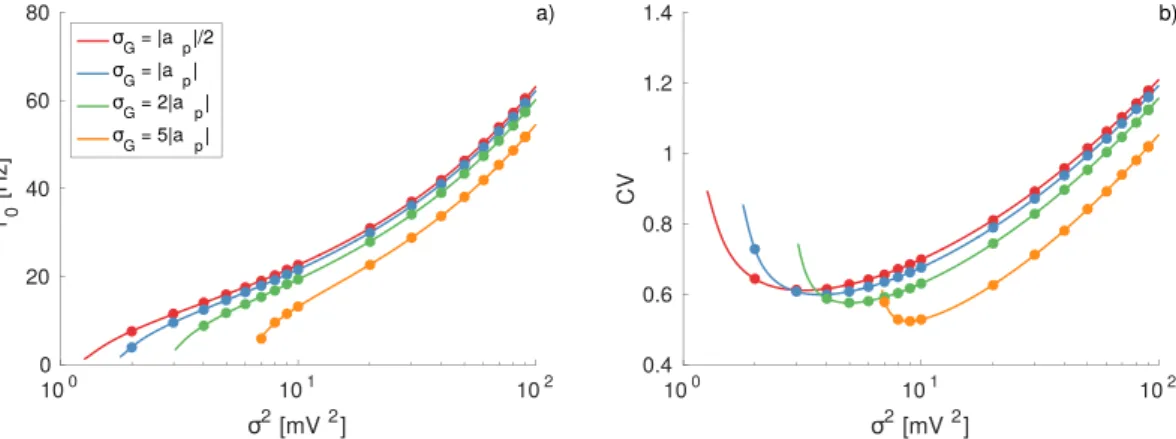
These conclusions are supported by the data reported in Fig. 4(a). In the figure are reported the average firing rate r0 for TGDs with different standard deviation σG and fixed position of the maximum at ap = −1 mV. For
increasing σG the neuronal activity decreases for corresponding noise amplitudes. Since the value of the skewness
asymmetry is also responsible for a shift of the position of the minimum of CV, associated to the CR phenome-non, towards larger σ2 and for a more regular firing activity observable at σ >σ
m
2 2, as shown in Fig. 4(b).
Figure 2. Firing time statistics for different IPSP distributions. Firing rate r0 and CV as a function of noise intensity for sub-threshold (μT = 9 mV) (a,b) and supra-threshold neurons (μT = 11 mV) (c,d). In all the panels
the symbols correspond to numerical simulations, the dashed black lines to the DA, calculated from Eqs (53) and (54), and the solid lines to the theoretical results reported in Eq. (17) and Eq. (27). The average IPSP amplitude is set to 〈|ai|〉 = 1 mV for all the distributions. For the TGD: the peak position |ap| and the width
σG of the distribution are equal (namely, ≈0.7766 mV). For the UD: l1 = 2ai and l2 = 0. Other parameters and simulation procedures as in Fig. 1.
Figure 3. Spike Train Spectra. (a) Normalized spike train spectra ωˆC( )/r0 for the same cases shown in
Fig. 1(a,b) for an effective input μT = 9 mV and noise intensity σ2 = 2 mV2; (b) Normalized spike train spectra
for the distributions considered in Fig. 2(a,b) for 〈|ai|〉 = 1, μT = 9 mV and σ2 = 4 mV2. In both panels, the
symbols correspond to the simulation results, while the continuous line to the theoretical estimations using Eq. (22). Simulated spectra were obtained by calculating the squared modulus of the Fourier transform of the spike train using a time trace of 64 s with 1 ms binning, and averaging over 10,000 realizations.
So far we considered as excitatory input a constant DC term, however the analytic approach here presented can be applied also for exponentially distributed excitatory amplitudes, namely Ae=exp(−a a a/ )/e e. We have
reported the results for this case for different inhibitory distributions in Fig. 5, the analytic estimations reproduce very well the numerical results both for the firing rate and the CV in an ample range of noise intensities. However, for small values of the noise intensity, the analytic results slightly deviates from the numerical values due to the fact that in the limit of small rates the numerical evaluation of the integrals entering in the expresssion of the generating function Z0 have problems of convergece. The effect due to the different IPSP distributions is analo-gous to the one observed with a constant DC excitatory term. The DA, conversely, is unable to capture the precise values of these two quantities. Once more, for the reported case in Fig. 5 where μT = 9 mV, the CR effect is present.
It is important to remark that, in the specific case of exponentially distributed amplitudes of the EPSP, the approach discussed in this article fails when an additional supra-threshold DC current is applied, namely for
μ0 > vth. A brief discussion in this regard will be provided in the concluding section.
Heterogeneous Sparse Networks.
The previous theoretical analysis of single neuron response to an external Poissonian input can find application also in the analysis of the dynamics of recurrent LIF heterogeneous networks with random sparse connectivity. For sparse networks, the spike-trains impinging a certain neuron can be assumed to be uncorrelated and Poissonian29, 35. Furthermore, similarly to what done in ref. 29, we can assumethat the spike-trains in the networks can be self-consistently described as Poissonian processes with firing rates
r0(μ(j)) related to the neuronal excitability μ(j) of each single neuron j.
For the sake of simplicity, we will consider a network of inhibitory neurons, where each neuron is character-ized by a different level of excitability {μ(j)} encompassing any excitatory external drive as well as the specific
Figure 4. Effect of the distribution asymmetry on the firing time statistics. (a) Average firing rate r0 as a function of the noise intensity for different values of the standard deviation of the Gaussian distribution σG as
indicated in the legend. (b) Coefficient of variation CV for the same cases depicted in (a). The reported data refer to TGDs with the peak located at |ap| = 1 mV and to an effective input μT = 9 mV. Symbols correspond
to numerical simulations, and the solid lines to the theoretical results reported in Eq. (17) and Eq. (27). Other parameters and simulation procedures as in Fig. 1
Figure 5. Firing time statistics for exponentially distributed EPSPs. Firing rate r0 (a) and CV (b) as a function of noise intensity for excitatory synaptic weights distributed exponentially with average amplitude 〈ae〉 = 〈|ai|〉 = 1 mV. In this figure excitatory and inhibitory spike trains are balanced, i.e Re = Ri, while the
effective input is sub-threshold, namely μT = μ0 = 9 mV. The symbols and lines have the same definition as in Fig. 2, as well as all the other parameters for the IPSP distributions and the numerical simulations.
characteristic of the considered neuron. Therefore, the dynamics of the j-th neuron in the network can be written as
∑
µ τ δ = − − + − v j v j j K C g k t t ( ) [ ( ) ( )] 1 ( ) ( ); (56) k jk i kwhere K ≪ N is the number of synaptic neighbors, Cjk is the connectivity matrix with entries 1 (0) if the k-th
neuron is connected (not connected) to neuron j. The amplitudes of the IPSP ai(k) = gi(k)/K < 0 associated to the
firing of the k-th neuron is assumed to be randomly distributed following some of the distributions previously introduced.
For the population dynamics we will give an estimate of the average firing rate via a self-consistent approach by assuming that in average each neuron receive a single Poissonian spike train with a rate =Ri r K0 and where
each IPSP has a random amplitude ai taken from a distribution Ai(a). An estimation of the average firing rate can
be obtained by solving the following implicit equation
∫
∫
τ µ µ µ = ∆ µ − r d P dc c F c cZ c r 1 ( ) ( ) ( , , ) ; (57) x 0 { } 0 0 0 1 Awhich is an extension to an heterogeneous network of Eq. (17) and where, as we have previously discussed, F(c) depends on the excitatory input and Z0 on the chosen IPSP distribution. It is important to stress that usually in inhibitory networks not all neurons are firing, but just a certain fraction n* will be active34, therefore the integral
reported in (57) is limited to these neurons, which are the one with higher excitability μ(j) ∈ {μA}. Furthermore
∫
µ µ∆ =
µ d P( )
{ }A is the support of the active neurons. Once the firing rates have been obtained self consistently
we can derive the coefficient of variation of each single neuron according to Eqs (26) and (27) and then to per-form the population average as follows
∫
µ µ µ = ∆ µ d P . CV 1 ( )CV( ) (58) { }AIn ref. 34 a theoretical approach to obtain self-consistently n*, r
0 and the average coefficient of variation CV has
been developed for constant IPSP, i.e. for δ-distribution. Here we extend such approach to more generic IPSP distributions, however we will limit to obtain the analytic estimations of r0 and CV. The values of n*, entering in the expressions for the average population rate and coefficient of variation, will be considered as parameter values obtained directly from the simulations. We have verified that the comparison with the numerical findings is very good for all the four considered IPSP distributions and for the whole considered range of average synaptic inputs 〈ai〉. For illustration purposes we present in Fig. 6(a,b) the average firing rate r0 and CV, for the two distributions
that have consistently presented larger differences between them, namely DD and ED, and for the DA. While it is evident that the DA overestimates r0 and CV already for 〈|ai|〉 > 0.5 mV, we observe that in the case of
heterogene-ous networks the differences among the variheterogene-ous IPSP distributions are quite limited at the level of the average firing rate r0 and CV. In order to investigate more in details the influence of different IPSP distributions on the
neuronal response, we have numerically estimated the probability distribution functions P(r0) of the single neu-ron firing rate r0 for DD and ED distributions. As shown in Fig. 6(c,d), the P(r0) obtained for the DD display a higher peak at low firing rate r0 with respect to the ED, while for higher firing rates they essentially coincide. This difference should be ascribed to the fact that sub-threshold neurons subject to IPSP trains with ED have a firing onset at definitely larger noise amplitudes than the ones subject to IPSPs with DD, while for supra-threshold neurons the differences are definitely less evident, as previously reported in Fig. 2(a,c). This explains also why the exam of the average firing rate does not reveal large difference between the two distributions, since the neurons with low firing rate contribute negligibly to the average activity. The influence of synaptic weight distributions on neuronal population dynamics has been usually examined in the context of homogeneous neuronal populations13,
17, where the single neuron response represents a good mean field approximation of the network dynamics.
However, from the present analysis it emerges that the heterogeneity in the single neuron excitability can render extremely difficult to distinguish among stimulations with different IPSP distributions.
As a final remark, we would like to stress that the reported approach works very well also for heterogene-ous sparse networks, provided that the collective dynamics is asynchronheterogene-ous. Otherwise, the presence of partial synchronization or of collective oscillations can induce correlations in the input spike trains, which cannot be accounted for with this approach. In particular, to avoid phase locking among the neurons the distribution P(μ) of the excitabilities should be sufficiently wide.
Conclusions
In this paper we have reported a theoretical methodology to obtain exact firing statistics for leaky integrate-and-fire neurons subject to discrete inhibitory noise, accounting for Poissonian trains of uncorre-lated post-synaptic potentials. Our results represent an extension to generic synaptic weights distribution of the approach developed in ref. 17 for exponentially distributed post-synaptic potentials. In particular, we report explicit results for the firing rate, the coefficient of variation and the spike train spectrum.
The comparison with numerical simulations reveals a very good agreement for all the considered distribu-tions over all the reported ranges of shot noise amplitude. Moreover, the method is also able to reproduce the average activity of an heterogeneous inhibitory neural network with sparse connectivity, by making use of a self-consistent mean field formulation. Conversely, the diffusion approximation3 (the most used theoretical
approach), gives a reasonable estimate of the firing time statistics for sufficiently small IPSP amplitudes, but the agreement rapidly degrades, and reveals large discrepancies already for amplitudes >0.5 mV, corresponding to physiologically relevant values8, 36, 37.
As a general result we observe that the firing statistics of single neurons is strongly influenced by the shape of the IPSP distributions. Distributions with longer tails lead to smaller firing rate and in general to more regular spike trains (for sufficiently large inhibition). For heterogeneous networks the value of the average IPSP has a noticeable influence on the firing activity of the neuronal population, while the shape of the synaptic weight distributions seem to have a really limited impact on the average properties of the network. However, differences induced by the IPSP distributions are still observable at the level of single neuron.
We have shown that the method works for any choice of IPSP amplitude distributions, however one has to be careful when dealing with the excitatory drive. We have shown that the agreement with numerical simulations is very good when the firing of the neuron is either promoted exclusively by a suprathreshold DC current or pro-vided by the stochastic arrivals of exponentially distributed EPSP amplitudes. In this latter case, an excitatory DC current can as well be present in addition to the EPSP trains, however the DC contribution must be strictly sub-threshold, namely, μ0 < vth. Whenever the two firing mechanisms are active at the same time (i.e. μ0 > vth), the
formulation reported in this paper is no more valid due to the inconsistency in the choice of the proper integra-tion limit x in Eq. (17). This limitation is illustrated in Fig. 7, where it is reported the response of a LIF neuron, subject to a supra-threshold excitatory DC current μ0 = 12 mV as well as to Poissonian spike trains of ED excita-tory and DD inhibiexcita-tory synaptic inputs. For small values of the noise intensity, the theoretical approach dramati-cally fails. In such a region the activity is almost exclusively current driven; i.e, the firing of the neuron promoted by the supra-threshold DC current is much faster than the arrival rate Re of the EPSPs. This can be confirmed by
the fact that in this regime the firing rate coincides with rt
0 in Eq. (51) for a tonic firing LIF neuron subject to a
constant DC current μT = μ0. As the noise intensity grows, corresponding to an increased rate Re of arrival of the
EPSPs, the numerical data approach the theoretical prediction obtained for exponentially distributed EPSPs. The
Figure 6. Firing time statistics for heterogenoeus networks as a function of the average synaptic weight. (a)
Average network frequency r0 and (b) average coefficient of variation CV as a function of the average synaptic weight 〈|ai|〉 for two representative IPSP distributions: DD (blue) and ED (green). Symbols correspond to
simulation values and solid lines to the theoretical results from Eqs (57) and (58). Dashed line denote the results of the DA. The numerically estimated probability distribution functions P(r0) of the single neuron firing rate r0 are also reported for the two considered IPSP distributions for two values of the average synaptic weight: namely 〈|ai|〉 = 0.04 (c) and 〈|ai|〉 = 0.4 (d). Simulations were performed with N = 400 neurons, K = 20 and a
distribution of the input currents uniformly chosen in the interval μ(j) ∈ [10, 11] mV. The time averages are calculated, after discarding an initial transient corresponding to 106 spikes, over the following 106 spikes. Silent neurons (those that do not emit any spike in the considered time lapse) are not included in the statistics. In all cases 〈|ai|〉 denotes the average value of the corresponding distribution.
crossover occurs for ≈Re 2r0t, indicating that the firing activity of the neuron is now mainly driven by the
sto-chastic component.
An interesting semi-analytic approach has been recently reported for excitatory shot noise in ref. 13. However, further progresses are required to achieve exact firing time statistics going beyond the diffusion approximation for generic distributions of instantaneous excitatory PSPs, as well as for more realistic neuronal models like the Exponential Integrate and Fire (EIF) neuron39 able to reproduce quite accurately the dynamics of cortical
neu-rons40. In particular, as shown in the Supplementary Information, the LIF neuron response is a limit case of
the EIF dynamics both within the diffusion approximation as well as for shot noise. Furthermore, the diffusion approximation fails also for the EIF to capture the neuronal firing statistics for sufficiently large IPSP amplitudes in particular at low noise intensities.
References
1. Destexhe, A., Rudolph, M. & Paré, D. The high-conductance state of neocortical neurons in vivo. Nature reviews neuroscience 4, 739–751, doi:10.1038/nrn1198 (2003).
2. Shadlen, M. N. & Newsome, W. T. The variable discharge of cortical neurons: implications for connectivity, computation, and information coding. The Journal of neuroscience 18, 3870–3896 (1998).
3. Ricciardi, L. M. Diffusion processes and related topics in biology vol. 14 (Springer Science & Business Media, 2013).
4. Tuckwell, H. C. Introduction to theoretical neurobiology: Volume 2, nonlinear and stochastic theories vol. 8 (Cambridge University Press, 2005).
5. Roxin, A., Brunel, N., Hansel, D., Mongillo, G. & van Vreeswijk, C. On the distribution of firing rates in networks of cortical neurons.
The Journal of neuroscience 31, 16217–16226, doi:10.1523/JNEUROSCI.1677-11.2011 (2011).
6. Song, S., Sjöström, P. J., Reigl, M., Nelson, S. & Chklovskii, D. B. Highly nonrandom features of synaptic connectivity in local cortical circuits. PLoS Biol 3, e68, doi:10.1371/journal.pbio.0030068 (2005).
7. Lefort, S., Tomm, C., Sarria, J.-C. F. & Petersen, C. C. The excitatory neuronal network of the c2 barrel column in mouse primary somatosensory cortex. Neuron 61, 301–316, doi:10.1016/j.neuron.2008.12.020 (2009).
8. Miles, R. Variation in strength of inhibitory synapses in the ca3 region of guinea-pig hippocampus in vitro. The Journal of Physiology
431, 659–76, doi:10.1113/jphysiol.1990.sp018353 (1990).
9. Mason, A., Nicoll, A. & Stratford, K. Synaptic transmission between individual pyramidal neurons of the rat visual cortex in vitro.
The Journal of Neuroscience 11, 72–84 (1991).
10. Barbour, B., Brunel, N., Hakim, V. & Nadal, J.-P. What can we learn from synaptic weight distributions? TRENDS in Neurosciences
30, 622–629, doi:10.1016/j.tins.2007.09.005 (2007).
11. DeWeese, M. R. & Zador, A. M. Non-Gaussian membrane potential dynamics imply sparse, synchronous activity in auditory cortex.
Journal of Neuroscience 26, 12206–12218, doi:10.1523/JNEUROSCI.2813-06.2006 (2006).
12. Buzsáki, G. & Mizuseki, K. The log-dynamic brain: how skewed distributions affect network operations. Nature Reviews Neuroscience
15, 264–278, doi:10.1038/nrn3687 (2014).
13. Iyer, R., Menon, V., Buice, M., Koch, C. & Mihalas, S. The influence of synaptic weight distribution on neuronal population dynamics. PLoS Comput Biol 9, e1003248, doi:10.1371/journal.pcbi.1003248 (2013).
14. Teramae, J.-n., Tsubo, Y. & Fukai, T. Optimal spike-based communication in excitable networks with strong-sparse and weak-dense links. Scientific Reports 2 (2012).
15. Collins, J., Chow, C. C. & Imhoff, T. T. et al. Stochastic resonance without tuning. Nature 376, 236–238, doi:10.1038/376236a0 (1995).
16. Gammaitoni, L., Hänggi, P., Jung, P. & Marchesoni, F. Stochastic resonance. Reviews of modern physics 70, 223–287, doi:10.1103/ RevModPhys.70.223 (1998).
17. Richardson, M. J. & Swarbrick, R. Firing-rate response of a neuron receiving excitatory and inhibitory synaptic shot noise. Physical
review letters 105, 178102, doi:10.1103/PhysRevLett.105.178102 (2010).
18. Burkitt, A. N. A review of the integrate-and-fire neuron model: I. homogeneous synaptic input. Biological cybernetics 95, 1–19, doi:10.1007/s00422-006-0068-6 (2006).
19. Burkitt, A. N. A review of the integrate-and-fire neuron model: Ii. inhomogeneous synaptic input and network properties. Biological
cybernetics 95, 97–112, doi:10.1007/s00422-006-0082-8 (2006).
20. Stein, R. B. A theoretical analysis of neuronal variability. Biophysical Journal 5, 173–94, doi:10.1016/S0006-3495(65)86709-1 (1965).
Figure 7. Firing time statistics for exponentially distributed EPSPs and supra-threshold DC current. Firing rate
r0 as a function of noise intensity for excitatory synaptic weights distributed exponentially and a supra-threshold DC current. All parameters as in Fig. 5 except for μT = μ0 = 12 mV. The dashed red horizontal line refers to the
rate rt
0 of the LIF neuron subject to constant current μT (Eq. (51)). Other symbols and lines have the same
21. Rauch, A., La Camera, G., Luscher, H.-R., Senn, W. & Fusi, S. Neocortical Pyramidal Cells Respond as Integrate-and-Fire Neurons to In Vivo Like Input Currents. J. Neurophys 90, 1598–1612, doi:10.1152/jn.00293.2003 (2003).
22. Jolivet, A., Rauch, A., Lüscher, H.-R. & Gerstner, W. Predicting spike timing of neocortical pyramidal neurons by simple threshold models. J Comput Neurosci 21, 35–49, doi:10.1007/s10827-006-7074-5 (2006).
23. Gerstner, W. & Kistler, W. M. Spiking neuron models: Single neurons, populations, plasticity (Cambridge university press, 2002). 24. Richardson, M. J. Spike-train spectra and network response functions for non-linear integrate-and-fire neurons. Biological
Cybernetics 99, 381–392, doi:10.1007/s00422-008-0244-y (2008).
25. Tuckwell, H. C. On the first-exit time problem for temporally homogeneous markov processes. Journal of Applied Probability 13, 39–48, doi:10.1017/S0021900200048981 (1976).
26. Giraudo, M. T. & Sacerdote, L. Jump-diffusion processes as models for neuronal activity. Biosystems 40, 75–82, doi: 10.1016/0303-2647(96)01632-2 (1997).
27. Kou, S. G. & Wang, H. First passage times of a jump diffusion process. Advances in applied probability 35, 504–531, doi:10.1017/ S0001867800012350 (2003).
28. Lindner, B., Schimansky-Geier, L. & Longtin, A. Maximizing spike train coherence or incoherence in the leaky integrate-and-fire model. Physical Review E 66, 031916, doi:10.1103/PhysRevE.66.031916 (2002).
29. Brunel, N. & Hakim, V. Fast global oscillations in networks of integrate-and-fire neurons with low firing rates. Neural. Comput. 11, 1621–1671, doi:10.1162/089976699300016179 (1999).
30. Amit, D. J. & Brunel, N. Model of global spontaneous activity and local structured activity during delay periods in the cerebral cortex. Cerebral cortex 7, 237–252, doi:10.1093/cercor/7.3.237 (1997).
31. Dummer, B., Wieland, S. & Lindner, B. Self-consistent determination of the spike-train power spectrum in a neural network with sparse connectivity. Frontiers in computational neuroscience 8, 10.3389/fncom.2014.00104 (2014).
32. Lindner, B., Garca-Ojalvo, J., Neiman, A. & Schimansky-Geier, L. Effects of noise in excitable systems. Physics Reports 392, 321–424, doi:10.1016/j.physrep.2003.10.015 (2004).
33. Pikovsky, A. S. & Kurths, J. Coherence resonance in a noise-driven excitable system. Physical Review Letters 78, 775–778, doi:10.1103/PhysRevLett.78.775 (1997).
34. Angulo-Garcia, D., Luccioli, S., Olmi, S. & Torcini, A. Death and rebirth of neural activity in sparse inhibitory networks. New Journal
of Physics. In Press, doi:10.1088/1367-2630/aa69ff (2017)
35. Brunel, N. Dynamics of sparsely connected networks of excitatory and inhibitory spiking neurons. J. Comput. Neurosci. 8, 183–208, doi:10.1023/A:1008925309027 (2000).
36. Buhl, E. H., Halasy, K. & Somogyi, P. Diverse sources of hippocampal unitary inhibitory postsynaptic potentials and the number of synaptic release sites. Nature 368, 823–828, doi:10.1038/368823a0 (1994).
37. Tepper, J. M., Koós, T. & Wilson, C. J. Gabaergic microcircuits in the neostriatum. Trends in neurosciences 27, 662–669, doi:10.1016/j. tins.2004.08.007 (2004).
38. Isope, P. & Barbour, B. Properties of unitary granule cell→purkinje cell synapses in adult rat cerebellar slices. The Journal of
neuroscience 22, 9668–9678 (2002).
39. Fourcaud-Trocmé, N., Hansel, D., van Vresswijk, C. & Brunel, N. How Spike Generation Mechanisms Determine the Neuronal Response to Fluctuating Inputs. J. Neurosci. 23, 11628–11640 (2003).
40. Badel, L. et al. Dynamic I–V curves are reliable predictors of naturalistic pyramidal-neuron voltage traces. J. Neurophysiol. 99, 656–666, doi:10.1152/jn.01107.2007 (2008).
Acknowledgements
We thank for useful discussions B. Lindner, G. Mato, A. Politi, G. Martelloni, MJE Richardson, M. Timme. This work has been partially supported by the European Commission under the program “Marie Curie Network for Initial Training“, through the project N. 289146, “Neural Engineering Transformative Technologies (NETT)“ and by the A*MIDEX grant (No. ANR-11-IDEX-0001-02) funded by the French Government “Programme Investissements d'Avenir” (D.A.-G. and A.T.). AT gratefully acknowledges a “VELUX Visiting Professor Grant“ from Villum Fonden that supported his stay at Aarhus University during the initial stages of this work in 2011. AI is supported by the Danish Council for Independent Research and the Villum Fonden. This work has been completed at Max Planck Institute for the Physics of Complex Systems in Dresden (Germany) as part of the activity of the Advanced Study Group 2016 entitled “From Microscopic to Collective Dynamics in Neural Circuits”.
Author Contributions
S.O. and D.A.-G. performed the numerical simulations. D.A.-G. and A.T. prepared the manuscript. All the authors developed the theoretical methods and reviewed the manuscript.
Additional Information
Supplementary information accompanies this paper at doi:10.1038/s41598-017-01658-8 Competing Interests: The authors declare that they have no competing interests.
Publisher's note: Springer Nature remains neutral with regard to jurisdictional claims in published maps and
institutional affiliations.
Open Access This article is licensed under a Creative Commons Attribution 4.0 International
License, which permits use, sharing, adaptation, distribution and reproduction in any medium or format, as long as you give appropriate credit to the original author(s) and the source, provide a link to the Cre-ative Commons license, and indicate if changes were made. The images or other third party material in this article are included in the article’s Creative Commons license, unless indicated otherwise in a credit line to the material. If material is not included in the article’s Creative Commons license and your intended use is not per-mitted by statutory regulation or exceeds the perper-mitted use, you will need to obtain permission directly from the copyright holder. To view a copy of this license, visit http://creativecommons.org/licenses/by/4.0/.