A Better Understanding of the Ecological Conditions for Leontopodium alpinum Cassini in the Swiss Alps

A Better Understanding of the Ecological Conditions

for Leontopodium alpinum Cassini in the Swiss Alps

Mélanie Ischer&Anne Dubuis&Roland Keller&

Pascal Vittoz

# Institute of Botany, Academy of Sciences of the Czech Republic 2014

Abstract Although Leontopodium alpinum is considered to be threatened in many countries, only limited scientific information about its autecology is available. In this study, we aim to define the most important ecological factors which influence the distribution of L. alpinum in the Swiss Alps. These were assessed at the national scale using species distribution models based on topoclimatic predictors and at the community scale using exhaustive plant inventories. The latter were analysed using hierarchical clustering and principal component analysis, and the results were interpreted using ecological indicator values. Leontopodium alpinum was found almost exclusively on base-rich bedrocks (limestone and ultramafic rocks). The species distribution models showed that available moisture (dry regions, mostly in the Inner Alps), elevation (mostly above 2,000 m a.s.l.) and slope (mostly >30°) were the most important predictors. The relevés showed that L. alpinum is present in a wide range of plant communities, all subalpine-alpine open grasslands, with a low grass cover. As a light-demanding and short species, L. alpinum requires light at ground level; hence, it can only grow in open, nutrient-poor grasslands. These conditions are met in dry conditions (dry, summer-warm climate, rocky and draining soil, south-facing aspect and/or steep slope), at high eleva-tions, on oligotrophic soils and/or on windy ridges. Base-rich soils appear to also be essential, although it is still unclear whether this corresponds to physiological or ecological (lower competition) requirements.

Keywords Alpine grasslands . Autecology . Phytosociology . Species distribution models . Switzerland

DOI 10.1007/s12224-014-9190-8

Electronic supplementary material The online version of this article (doi:10.1007/s12224-014-9190-8) contains supplementary material, which is available to authorized users.

M. Ischer

:

:

Department of Ecology and Evolution, University of Lausanne, Biophore Building, CH-1015 Lausanne, Switzerland

e-mail: pascal.vittoz@unil.ch R. Keller

Introduction

Leontopodium alpinum is a perennial herbaceous hemicryptophyte that grows 8–20 cm high (Aeschimann et al. 2004) and is characterized by 2–10 small yellow capitula surrounded by white and woolly bracts visited by a wide range of insects (Erhardt 1993). Its colour, shape, rarity and legendary inaccessibility have conferred upon it a high symbolic value in alpine regions. Indeed, this species is prized by tourists and botanists (Erhardt1993); its common name, Edelweiss, comes from German and means noble (edel) and white (weiss; Dweck2004).

Leontopodium alpinum is mostly found in alpine areas, ranging from the Pyrenees to the Central Balkans in Bulgaria (Wagenitz1979). The genus is native to the Tibetan Plateau and might have migrated during the Pleistocene, when a continual distribution between Asia and Europe was possible (Blöch et al. 2010). This species has been mostly studied with regard to its pharmaceutical properties (antibacterial, anti-inflammatory and analgesic properties; Dobner et al. 2003, 2004; Speroni et al. 2006). In Switzerland, L. alpinum has been domesticated (var. helvetica) and is now cultivated to produce anti-aging creams, sunscreens and liquor (Carron et al.2007) or for ornamental purposes (Sigg2008).

Despite the symbolic value of L. alpinum in the Alps, limited scientific information about its autecology is available, with the literature being mostly restricted to descrip-tive floras based on expert knowledge. We could not find any descripdescrip-tive study clearly based on detailed field data. Wagenitz (1979) and Oberdorfer and Müller (1990) indicate that this plant is a light-demanding species found in sunny, rocky grasslands or on cliffs (ledges or crevices) from 1,600 m a.s.l. to 2,350 m a.s.l. (–3,000 m a.s.l.) in regions with warm summers, on base-rich, mostly calcareous, neutral and mainly humus-rich soils. According to Delarze and Gonseth (2008), this species is found in two distinct phytosociological alliances in Switzerland, Seslerion and Elynion, both of which are characterized by alkaline to neutral calcareous soils. Seslerion is distributed on sunny slopes between 1,000 m a.s.l. and 2,400 m a.s.l., on dry and stony soils. Elynion is restricted to windy ridges between 2,000 m a.s.l. and 3,000 m a.s.l., which are only partly protected by snow in winter. Wagenitz (1979) and Oberdorfer and Müller (1990) add Potentillion caulescentis on limestone cliffs as a possible alliance. Rey et al. (2011) recently published a synthesis based on previous floras and the extensive experience of the main author, adding to the previous descriptions a prefer-ence for a subcontinental climate on slightly dry, oligotrophic soils, with a pH range of 5.5–8.

Although L. alpinum is considered as of “Least Concern” on the Swiss Red List (Moser et al.2002), it is not a widespread species. Some populations include hundreds of plants; however, most of the populations are restricted to a few individuals, and the species is far from being present in all Seslerion or Elynion areas in the Alps. Unfortunately, no monitoring of its populations exists, though many botanists have an impression of decreasing populations. Indeed, this species is considered to be endangered and is protected in most countries or regions where it occurs (cf. review of its status in Rey et al. 2011 and for Switzerland at www.infoflora.ch). Collection by tourists for the species’ beauty and symbolic value is most likely responsible for the population decreases (Jean 1947; Wagenitz 1979; Rey et al. 2011).

In order to ensure optimal conservation of L. alpinum, it is important to identify dominant ecological factors in its distribution and therefore to back up the existing expert knowledge with field measurements (evidence-based conser-vation; e.g. Arlettaz et al.2010). Distribution models are effective tools to obtain reliable information on the ecology of species (Guisan and Zimmermann 2000) because they allow detecting and ranking ecological factors affecting species fitness (Elith and Leathwick 2009). Such models produce faithful habitat suit-ability maps (Le Lay et al. 2010), and their use is possible with rare or uncommon species (Engler et al. 2004). Exhaustive phytosociological relevés, which are numerous in Switzerland (Schaminée et al.2009), offer a quick way to obtain data on many populations, with partner species giving indirect indications of ecological conditions (Deil 2005; Vittoz et al. 2006).

This study aimed to improve our knowledge regarding the necessary ecological conditions for L. alpinum in the Swiss Alps. In particular, we aimed to identify the most important ecological factors explaining the distribution of this species and to obtain a complete overview of the habitats in which the plant can grow. For this, (1) we modelled species distribution on the basis of 344 recorded occurrences, geology and five topoclimatic predictors to identify important ecological factors at the national scale and produce a map of potential habitats, and (2) performed clustering and multivariate analyses on 249 exhaustive plant inventories, interpreted with the help of ecological indicator values, to study the species ecological range at the community scale.

Material and Methods Study Area

The entire area of the Swiss Alps, representing 60 % of Switzerland, was considered in this study. Due to their proximity to the Atlantic Ocean and the Mediterranean Sea, the Outer Alps are characterized by a wet, suboceanic climate. Conversely, some valleys in the Inner Alps are protected from rainfall by high mountains and experience a dry, subcontinental climate.

Floristic Data

The existing data on L. alpinum were collected, either in the form of exhaustive species lists (phytosociological relevés) or from isolated observations. Relevés were collected from the literature (Braun-Blanquet1969; Galland1982; Reinalter2004; Steiner2002), from personal data obtained in previous projects (Randin et al. 2010) and from unpublished data (M. Ischer, J.-L. Richard, M. Schütz, R. Keller). All Swiss relevés were retained, without consideration of the size of the inventoried plot or the availabil-ity of exact coordinates. The vascular plant nomenclature is according to Aeschimann et al. (2004).

Isolated observations were mainly provided by Info Flora (Swiss Floristic Network; www.infoflora.ch/) and completed by occurrences in relevés. Only observations with a horizontal accuracy of 100 metres or less were retained for the models. 174 of the 344 available occurrences were from the relevés.

Environmental Data

The species’ distribution in relation to geology was evaluated by counting the number of L. alpinum occurrences in each geological category. We used a geotechnical map at a 1 : 200,000 scale (Swiss Geotechnical Commission, www.sgtk.ch) in which the substrates are divided into 30 categories defined by bedrock type or granulometry for recent deposits. These categories were simplified into four categories: purely calcareous bedrocks, mixed bedrocks potentially with limestone (e.g., moraines, alluvial deposits, conglomerates), ultramafic bedrocks and base-poor bedrocks (e.g., granite, quartzite).

In the species distribution models, we used three climatic and two topographic predictors, corresponding to the ecological factors susceptible to influence L. alpinum distribution on the basis of previous descriptions and generally considered as important and complementary ecological variables to explain species distribution in mountain environments (Körner2003). The climatic predictors were calculated based on tem-perature and precipitation data recorded by MeteoSwiss (www.meteoswiss.ch) and interpolated with a 25 m resolution digital elevation model (see Zimmermann and Kienast1999for methodology). We used the mean temperature for the growing season (June to August, in °C), the average moisture index over the growing season (average value of the balance between precipitation and potential evapotranspiration in mm/day) and the sum of solar radiation for the growing season (in kJ · m–2 · yr–1). The topographic predictors were derived from the digital elevation model. We used the slope (in degrees) and topographic position (an integrated measure of topographic features; Zimmermann et al. 2007); positive values of topographic position indicate ridges whereas negative values indicate valleys.

Species Distribution Models

To restrain the study area considered in the models to plausible areas for L. alpinum, a mask was created by removing urbanized areas, glaciers and lakes. Moreover, only elevations higher than 1,300 m a.s.l. were retained because no current occurrence is reported at lower elevations and the large majority of observations are above 1,500 m a.s.l. Out of the 344 available observations, we randomly selected occurrences separated by a minimum distance of 250 metres to avoid spatial autocorrelation. This selection was repeated 20 times, to test for potential differences in the models due to occurrence selection, retaining an average of 214 occurrences (see Appendix 1 in Electronic Supplementary Material for distances between occurrences before and after disaggre-gation). Absences were not directly available because occurrences were mainly obser-vations of presences only, without recorded absences. The use of other phytosocio-logical relevés in the Swiss Alps could have provided real absences, but these data are not digitalized or they issued from regional research projects and absences would have been aggregated, bringing biases in models. For these reasons, we used pseudo-absences to calibrate the models (Engler et al. 2004). Using Hawth’s Analysis Tools in ArcGIS (2004), we randomly generated 10,000 pseudo-absences in the entire study area, as defined in the preceding paragraph. We used all the pseudo-absences during the model calibration but gave to each of them a weight equal to the number of occurrences divided by 10,000, as recommended by Wisz and Guisan (2009) and Barbet-Massin et al. (2012).

The models were computed using the library BioMod (Thuiller et al.2009) in R (v.2.14.1; R Development Core Team 2011). Four model types were computed to obtain a reliable probability regarding the presence of L. alpinum: generalized linear models (GLM; McCullagh and Nelder1989) with a polynomial term and a stepwise procedure (computed with Akaike information criteria, AIC), generalized additive models (GAM; Hastie and Tibshirani1990) using a spline function with a degree of smoothing of 4, generalized boosting models (GBM; Ridgeway1999; Friedman et al. 2000) with 2,000 trees and random forest (RF; Brieman2001).

As no independent data were available to evaluate the models, we used a split-sample procedure, and 70 % of the data (presences and pseudo-absences) were randomly chosen and used for model calibration, with 30 % used for model evaluation. This procedure was repeated five times for each model type and for each of the 20 datasets of occurrence selection. For each data split, the predictive performance of the models was evaluated with two frequently used metrics: the area under the curve (AUC) of a receiver operating characteristic plot (ROC; Ogilivie and Creelman1968) and the Boyce index (Boyce et al.2002). The AUC varies from 0.5 (random predic-tions) to 1 (perfect models); a model is considered reliable with AUC higher than 0.7 (Swets1988). The Boyce index varies between−1 (counter predictions) and 1 (perfect predictions). This index is particularly adapted for our data as it is calculated based on presences only, independently of pseudo-absences (Hirzel et al.2006).

As proposed in BioMod (Thuiller et al. 2009), the relative importance of each predictor in a model was calculated by randomizing one predictor and projecting the model with the randomized variable while keeping the other predictors unchanged. The results of the model containing the randomized predictor were then correlated with those of the original model. The importance of the predictor was calculated as one minus this correlation (consequently, the higher the value is, the more important is the variable for the model quality). For each model and for each of the 20 datasets of occurrence selection, the calculation of predictor importance was repeated with five datasets of randomized values.

To produce the most reliable map of potential habitat, we used an ensemble forecasting, as recommended by Araújo and New (2007), with the final set of models calibrated using one of the randomly selected dataset with 214 occurrences and 10,000 weighted pseudo-absences. The results of the four models (GLM, GAM, GBM and RF) were average weighted by their respective AUC. The probabilities of presence predict-ed by the ensemble model were transformpredict-ed into presence-absence data with an optimized threshold maximizing the model sensitivity and specificity (Liu et al. 2005). The projection of the ensemble model was finally restricted to the three geological categories on which L. alpinum was most commonly observed (see the Resultssection).

Analyses of Relevés

All the subsequent analyses of the 249 relevés were realized following the elimination of rare species (<3 occurrences) and transformation of the cover indices (Braun-Blanquet1964), as follows: r = 1, + = 2, 1 = 3, 2 = 4, 3 = 5, 4 = 6 and 5 = 7.

To distinguish groups of phytosociological relevés, a hierarchical clustering analysis was performed using the chord distance and Ward’s minimum variance clustering

method (Borcard et al.2011). The optimal number of groups was defined according to Mantel correlation coefficients between the distance matrix and binary matrices (0 if relevés are in the same group, 1 otherwise) computed from the dendrogram sectioned at various levels (see the function in R given by Borcard et al.2011, p. 71). Differential species in the groups were selected by calculating their indicator values (Dufrêne and Legendre1997).

The ecological conditions of each group were documented by the eight ecological indicator values attributed to species by Landolt et al. (2010). The median value was calculated for each relevé and each indicator value. However, to obtain more informa-tive values than the habitual median limited to the indicator classes, the medianμ was calculated with the following formula based on the 50 % value of a cumulative frequency curve (Ellenberg1991):

μ ¼ m þ wðn=2Þ−nm

nx

where m is the lower limit of the median class (here, the intermediate value between the median class and the previous one), w is the width of the classes (0.5 for T and F; 1 for L, K, R and N; 2 for D and H; see Table2for abbreviations), n is the number of species in the relevé, nmis the number of species with an indicator value lower than the median class, and nx is the number of species with an indicator value similar to the median class.

A principal component analysis (PCA), after a Hellinger transformation of the data (Legendre and Gallagher2001), was computed to study the distribution of the groups along floristic gradients. The ecological indicator values (Landolt et al.2010) were passively projected using the correlation between the median ecological values of each relevé and its scores on corresponding axes (Wohlgemuth2000).

These analyses were computed using R software (R Development Core Team2011) with the libraries vegan (clustering, Hellinger transformation, PCA) and labdsv (indi-cator values of the species). The nomenclature of the phytosociological alliances follows Delarze and Gonseth (2008), and the names of associations were conserved from the authors of the relevés (not all the relevés were classified).

Results

Out of the 344 available occurrences, 242 were on pure calcareous bedrocks, 49 on mixed bedrocks, 42 on ultramafic bedrocks and 11 on base-poor bedrocks. The distribution of L. alpinum occurrences in relation to ecological variables are summa-rized in Appendix2in Electronic Supplementary Material.

Species Distribution Models

The evaluation values obtained for the four modelling techniques and the 20 datasets (random selection of presences) after the split-sample procedure resulted in a mean AUC value of 0.81±0.01 and a mean Boyce index of 0.90±0.18. The four modelling techniques and the 20 datasets produced predictions of similar quality. As predictions

with AUC values were above 0.8 and Boyce index values close to 1, models can be qualified as good and trustworthy (Araújo et al.2005).

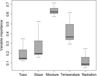
The most important predictor for modelling the distribution of L. alpinum was the average moisture index (Fig.1), followed by the summer temperature, the slope and the topographic position. Solar radiation was the least important predictor. The response curves of the models showed that the optimal value for the moisture index was less than 5 mm/day, which corresponds to dry conditions for the Alps (Fig.2). The suitability of habitat increased with decreasing mean temperature (i.e., with increasing elevation) and increasing slope.

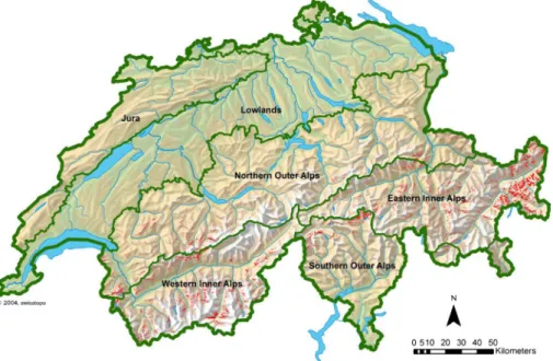
The map of predicted potential habitats showed that the Inner Alps are the most suitable area for L. alpinum, with isolated possible regions in the Outer Alps (Fig.3and Appendix3 in Electronic Supplementary Material). In summary, typical sites where L. alpinum can grow are in dry areas, at high elevations and on steep slopes.

Clustering and Principal Component Analysis of the Relevés

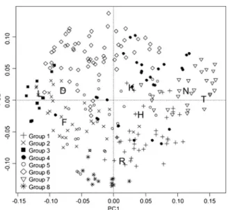
The first axis of the PCA explained 10.1 % of the variance, and the ecological indicator values pointed to a temperature and light gradient along this axis (Fig.4), extending from a heliophilous pole on the left side to a thermophilic pole on the right side. The second axis explained 7.4 % of the variance and was associated with a gradient of soil pH.

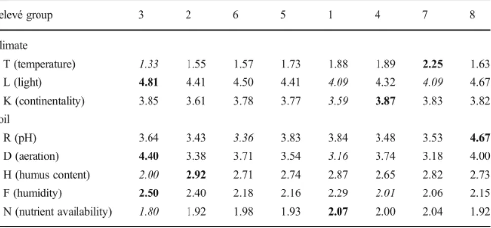
Eight groups of relevés were retained in the clustering analysis (Table 1). The median ecological indicator values (Table2) showed high ranges between the groups for soil pH (3.36–4.67, neutral to alkaline), soil aeration (3.16–4.40, moderate to good aeration), temperature (1.33–2.25, lower subalpine to alpine belts) and humus content (2.00–2.92, little to moderate). Moderate ranges of values were observed for the light conditions (4.09–4.81, well-lit sites to almost full light) whereas small ranges were found for humidity (moderately dry to fresh), continentality (subcontinental) and nutrient availability (infertile).

Fig. 1 Importance of each predictor used in the models: a high value (like moisture) indicates an important influence of the predictor in the models. Topo, topographic position; Slope, slope in degrees; Moisture, difference between precipitation and potential evapotranspiration over the growing season (June–August); Temperature, mean temperature for the growing season; Radiation, sum of solar radiation for the growing season

Group 3 contained the most heliophilous relevés under the coldest conditions and were situated on humus-poor soils but with good aeration (Table2). This group was differentiated by scree and rock species (Saxifraga oppositifolia, Carex rupestris,

Fig. 2 (a) Response curves for Leontopodium alpinum with GAM for the three most important predictors (the response curves for the other models showed similar trends) and (b) frequency distribution of the same predictors in the Swiss Alps. See Fig.1for the predictor abbreviations and Appendix2 in Electronic Supplementary Material for the distribution of L. alpinum occurrences in relation to all predictors

Fig. 3 Predicted habitat suitability map of Leontopodium alpinum (red areas) in the Swiss Alps (map from SwissTopo;www.swisstopo.admin.ch). Other colours correspond to elevation (greenish – <600 m a.s.l.; beige– 600–2,500 m a.s.l., white – >2,500 m a.s.l.). The map can be enlarged from the Appendix3in Electronic Supplementary Material

Herniaria alpina). Previous classifications of these relevés were mainly attributed to Herniarietum alpinae Zollitsch 1968 found on screes of calcareous slates (Drabion hoppeanae). Close to this group, group 2 shared Elyna myosuroides (highest frequency in this group) with two other Elynion species (Ligusticum mutellinoides, Arenaria ciliata). This group had the most humus-rich soils. The previously classified relevés were mostly attributed to Elynetum myosuroidis Rübel 1911 (Elynion), corresponding to alpine windy ridges.

At the other extreme of the light-temperature gradient, group 7 corresponded to the warmest and least lit (densest grass cover) conditions, and was differentiated by species belonging to continental steppes (Stipo-Poion: Carex humilis, Koeleria macrantha, Pulsatilla halleri, Erysimum rhaeticum) and other species from dry, thermophilous grasslands (e.g., Euphorbia cyparissias, Teucrium montanum, Dianthus sylvestris, Plantago serpentina, Galium lucidum). Almost all of these relevés are from the Zermatt region, in the Inner Alps, and were attributed to Astragalo leontini-Seslerietum Richard 1985, which is an association representing the dry, continental wing of Seslerion (Steiner2002). Group 1 is similarly characterized by poorly lit conditions and moderate soil aeration but colder conditions. All of the differential species (Senecio doronicum, Carex sempervirens, Anthyllis vulneraria subsp. alpestris, Festuca violacea aggr.) are typical of calcareous, alpine grasslands (Seslerion). The previously classified relevés were attributed to Seslerio-Caricetum sempervirentis Br.-Bl. in Br.-Bl. et Jenny 1926, the central association of the Seslerion.

The largest group (6) showed the lowest soil pH (R), corresponding to a mixture of calcicolous species (e.g., Draba aizoides, Oxytropis helvetica) and species colonizing neutral to weakly acidic soils (e.g., Artemisia glacialis, Veronica fruticans). Carex curvula s.l. is problematic, as it contains an acidophilous taxon (C. curvula s.str.) and

Fig. 4 Principal component analysis with passive projection of the ecological indicator values (Landolt et al.2010) for climate factors (T– temperature; K – continentality; L – light) and soil characteristics (N – nutrient availability; H – humus content; D – aeration; F – humidity; R – pH). The relevés are represented by symbols related to the groups obtained via clustering analysis (see Table1). Axes 1 and 2 explain 10.1 % and 7.4 % of the variance, respectively

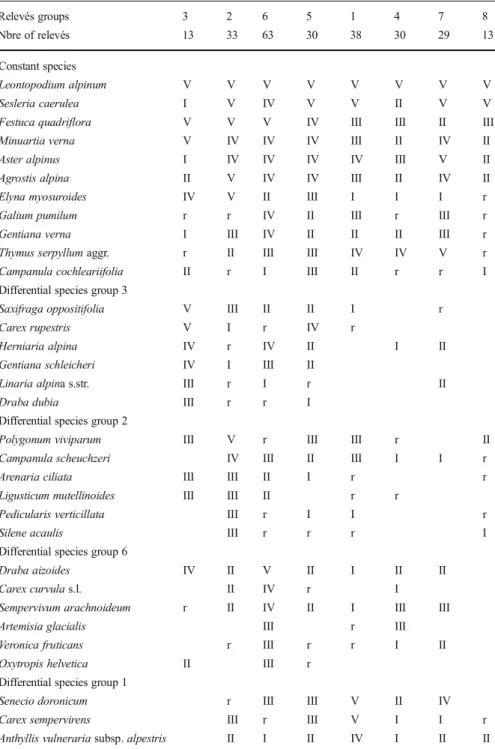
Table 1 Synthetic table of the clustering analysis. Eight groups of relevés were retained, and the species were classified based on their indicator values for the groups. The groups are approximately ordered following axis 1 of the PCA (see Fig.4). Only species present in at least 40 % of the relevés of one group are retained in this table (see Appendix5in Electronic Supplementary Material for the complete table). Species frequency in each group is given by a Roman numeral: V– species frequency >80 %; IV – 60–80 %; III – 40–60 %; II – 20–40 %; I– 10–20 %; r – <10 % Relevés groups 3 2 6 5 1 4 7 8 Nbre of relevés 13 33 63 30 38 30 29 13 Constant species Leontopodium alpinum V V V V V V V V Sesleria caerulea I V IV V V II V V

Festuca quadriflora V V V IV III III II III

Minuartia verna V IV IV IV III II IV II

Aster alpinus I IV IV IV IV III V II

Agrostis alpina II V IV IV III II IV II

Elyna myosuroides IV V II III I I I r

Galium pumilum r r IV II III r III r

Gentiana verna I III IV II II II III r

Thymus serpyllum aggr. r II III III IV IV V r Campanula cochleariifolia II r I III II r r I Differential species group 3

Saxifraga oppositifolia V III II II I r

Carex rupestris V I r IV r

Herniaria alpina IV r IV II I II

Gentiana schleicheri IV I III II

Linaria alpina s.str. III r I r II

Draba dubia III r r I

Differential species group 2

Polygonum viviparum III V r III III r II

Campanula scheuchzeri IV III II III I I r

Arenaria ciliata III III II I r r

Ligusticum mutellinoides III III II r r

Pedicularis verticillata III r I I r

Silene acaulis III r r r I

Differential species group 6

Draba aizoides IV II V II I II II

Carex curvula s.l. II IV r I

Sempervivum arachnoideum r II IV II I III III

Artemisia glacialis III r III

Veronica fruticans r III r r I II

Oxytropis helvetica II III r Differential species group 1

Senecio doronicum r III III V II IV

Carex sempervirens III r III V I I r

Table 1 (continued)

Relevés groups 3 2 6 5 1 4 7 8

Nbre of relevés 13 33 63 30 38 30 29 13

Festuca violacea aggr. r II I III r I

Phyteuma orbiculare r III

Scabiosa lucida r III

Differential species group 7

Bupleurum ranunculoides s.str. r r II I III V

Euphorbia cyparissias r II r II II V

Carex humilis r I II r V

Oxytropis campestris s.str. II II I II III IV

Dianthus sylvestris r r r III IV

Acinos alpinus r I r II II IV

Hieracium pilosella I I r II IV

Koeleria macrantha r II IV

Carlina acaulis subsp. caulescens r r I II I IV

Teucrium montanum r I r I IV r

Astragalus australis r I I II III

Plantago serpentina r r r II III

Pulsatilla halleri I r r II III

Erysimum rhaeticum r I II III

Campanula rotundifolia r I I I III

Trifolium montanum r r r r III

Astragalus leontinus r r I III

Briza media r I r III

Carex caryophyllea r r r III

Galium lucidum r r I III

Dactylis glomerata r III

Linum catharticum I III

Differential species group 8

Dryas octopetala II r I II V

Saxifraga caesia r I r V

Carex mucronata r r r I r IV

Gentiana clusii I I II IV

Carex firma I r IV

Crepis kerneri r III

Other species

Helianthemum alpestre II II IV III II III V

Carduus defloratus s.l. r I I IV r IV r

Galium anisophyllon r III IV III II I IV

Euphrasia salisburgensis I r II III r II I

Sedum atratum III I I I II I r

Gypsophila repens I r III II I III r

a calcicolous taxon (C. curvula subsp. rosae), though the exact taxon was not always indicated. However, 38 of the 39 precisely identified occurrences were C. curvula subsp. rosae. Three quarters of the relevés were previously attributed to Artemisio glacialis-Festucetum pumilae Richard 1985, a pioneer association of Seslerion on little-developed soils, rich in gravel and sand, partly unstable, in the Inner Alps (Steiner 2002), whereas one quarter was attributed to Elynetum myosuroidis.

Groups 4 and 5 presented intermediate compositions, without any frequent differ-ential species and showing median ecological values mostly around the middle of the

Table 1 (continued)

Relevés groups 3 2 6 5 1 4 7 8

Nbre of relevés 13 33 63 30 38 30 29 13

Helianthemum nummularium s.l. I II II V II V

Festuca ovina aggr. I II II II III IV

Lotus corniculatus aggr. r I I III I IV

Cerastium arvense subsp. strictum r III I I III II Gentiana campestris s.str. II I I III r I

Hieracium villosum r r III r II I

Globularia cordifolia r II II II III II

Juniperus communis subsp. nana r I II II I III

Silene exscapa III II II r I

Euphrasia alpina r II I II III

Anthyllis vulneraria subsp. valesiaca III II r I III

Leucanthemum adustum r III r III

Mean number of species 16.6 29 29.3 24.7 35.1 24.6 40.8 14.6

Table 2 Median ecological indicator values (Landolt et al.2010) of the groups of relevés. The groups are ordered following axis 1 of the PCA (Fig.4). The highest value of each indicator is in bold and the lowest in italics

Relevé group 3 2 6 5 1 4 7 8 Climate T (temperature) 1.33 1.55 1.57 1.73 1.88 1.89 2.25 1.63 L (light) 4.81 4.41 4.50 4.41 4.09 4.32 4.09 4.67 K (continentality) 3.85 3.61 3.78 3.77 3.59 3.87 3.83 3.82 Soil R (pH) 3.64 3.43 3.36 3.83 3.84 3.48 3.53 4.67 D (aeration) 4.40 3.38 3.71 3.54 3.16 3.74 3.18 4.00 H (humus content) 2.00 2.92 2.71 2.74 2.87 2.65 2.82 2.73 F (humidity) 2.50 2.40 2.18 2.16 2.29 2.01 2.06 2.15 N (nutrient availability) 1.80 1.92 1.98 1.93 2.07 2.00 2.04 1.92

ranges (Table2). The relevés were previously attributed to various associations: Artemisio glacialis-Festucetum pumilae, Seslerio-Caricetum sempervirentis, Androsacetum alpinae Br.-Bl. 1918 (fine screes of siliceous or ultramafic rocks, in Androsacion alpinae), Caricetum fimbriatae Richard 1985 (screes of ultramafic rocks, in Caricion curvulae), Androsacetum helveticae Br.-Bl. in Br.-Bl. & Jenny 1926 (alpine calcareous cliffs, in Potentillion caulescentis) or Potentillo caulescentis-Hieracietum humilis Br.-Bl. 1933 (montane-subalpine calcareous cliffs, in Potentillion caulescentis). All these associations are linked to rocky conditions with a low vegetation cover.

Lastly, group 8 was separated along the second axis of the PCA (Fig.4) and was characterized by the highest soil pH and was differentiated by six species found on rocky, open grasslands on limestone (Dryas octopetala, Saxifraga caesia, Carex mucronata, Gentiana clusii, Carex firma, Crepis kerneri). All of the previously classi-fied relevés were attributed to Caricetum firmae Rübel 1911, with rocky, calcareous grasslands in the alpine belt (Caricion firmae).

In summary, L. alpinum was observed in a broad range of phytosociological alliances (see Appendix 4 in Electronic Supplementary Material), all corresponding to subalpine-alpine communities on base-rich bedrocks, with a low to very low grass cover, on nutrient-poor, dry to fresh soils, among apparent rocks or on ridges.

Discussion

Significance of the Results

In this study, we investigated the autecology of Leontopodium alpinum to obtain a better understanding of its distribution in the Swiss Alps. The collected relevés were realized by different authors within the context of vegetation studies, mainly aiming to classify plant communities. Hence, we can consider them not to be biased toward particular conditions linked to L. alpinum growth. However, there is a regional bias, as approximately half of the 249 available relevés were from the Zermatt region, which is a particularly interesting region for the flora and plant communities and has been investigated extensively (Richard1991; Steiner2002). Nevertheless, the other available relevés are well distributed throughout the Swiss Alps, including the Outer Alps; altogether, they likely represent most of the ecological range of the species in Switzerland.

Ecological Conditions for L. alpinum

As indicated in previous descriptions (Wagenitz1979; Oberdorfer and Müller1990), L. alpinum was mostly observed on limestone, with 85 % of the occurrences on pure calcareous bedrocks or on mixtures containing limestone (e.g., moraines). However, other basic cations can replace calcium, as 12 % of the observations were on ultramafic bedrocks, previously only mentioned by Wagenitz (1979). Conversely, the species avoids siliceous bedrocks, with only 3 % of the occurrences, whereas this type of rocks represents 39 % of the Swiss Alps above 1,300 m a.s.l. As contamination by closely located limestone cannot be excluded for some of these rare occurrences, the proportion of occurrences on siliceous rocks is certainly lower. A soil map would have

probably given better results in the models. The high median ecological indicator value for soil pH (R) for all the groups of relevés (Table 2) confirmed the geological observations. However, this indicator also showed the highest variation among the groups, extending from weakly acid to alkaline soils. This corresponds to the pH of 5.5–8 reported by Rey et al. (2011) and indicates that the soil is consistently base-rich but can be completely decarbonated.

Another constant factor for all the relevés is the low grass cover, with only communities of open grasslands. L. alpinum is a light-demanding species (Wagenitz 1979), with most of the leaves in a rosette on the ground, and it most likely does not tolerate competition by other species. The importance of light at the ground level is shown by the constant species (Table 1; Sesleria caerulea, Festuca quadriflora, Minuartia verna, Aster alpinus and Agrostis alpina), which are all heliophilous (Landolt et al.2010), and by the median ecological value for light above 4 (well lit to full light) for all the groups of relevés. This low grass cover is provided by rocky conditions, sometimes in pioneer communities on slightly unstable screes, or by other harsh conditions limiting plant growth (see below). Although the species is indicated as growing in sunny conditions (Oberdorfer and Müller1990), solar radiation was not important as a predictor in the models, which most likely means that the aspect alone is not a constraint, with some stands occurring on a north aspect, and that a south-facing slope may be a way to limit plant growth through dry conditions.

Indeed, the most important predictor in the models was a low moisture index, translating into a preference for regions with an approximate balance between rainfall and potential evapotranspiration or even with a water deficit. In Switzerland, this corresponds to the subcontinental climate of the Inner Alps, as indicated by Rey et al. (2011), though the species is present in wetter regions as well. This finding is in agreement with the median ecological indicator values for continentality (K, sub-continental climate) and for soil humidity (F), ranging between moderately dry to fresh. Previously, Wagenitz (1979) characterized soil humidity for L. alpinum as relatively dry. The moderate to good aeration of the soil (indicator value D) can be considered to be a contribution to the good water drainage.

Temperature was the second most important predictor in the models, with a higher suitability for mean summer temperatures below 10°C, corresponding approximately to elevations >2,000 m a.s.l. This preference for high elevations has long been clear, though some isolated observations in lowlands have been reported (e.g., 220 m a.s.l. in Slovenia and 470 m a.s.l. in a Swiss wetland; Wagenitz1979; Rey et al. 2011). In addition, L. alpinum can grow with highly thermophilous species (e.g., Galium lucidum, Astragalus monspessulanus and Phleum phleoides which optimally grow in the warm colline belt; Landolt et al.2010), and is cultivated in the montane belt. This could indicate that low temperatures are not essential for this species, but indirectly help by limiting competition. The fundamental niche of L. alpinum related to the tempera-ture gradient is probably much larger than its realized niche.

Leontopodium alpinum has the reputation of growing in sites that are not easily accessible, on cliffs or steep slopes. However, slope had a low importance in models and its reputation is certainly overrated, with some large populations still easily accessible on weak slopes, although far away from villages. Wagenitz (1979) and Rey et al. (2011) indicated that this distribution corresponds to the populations remain-ing after decades of over-collection for the tourism market, but cliffs and steep slopes

could also be helpful in restricting competition by providing dryer conditions and continuous erosion.

Overall, the projection of the ensemble model predicted the suitable habitat (realized niche; Jiménez-Valverde et al.2008) of L. alpinum to mainly fall within the Inner Alps, with only isolated potentially favourable regions occurring in the Northern and Southern Outer Alps, though limestone is by far the dominant bedrock in the Northern Outer Alps. Moreover, the community analysis showed that the most important factor for the growth of this plant is certainly the light at the ground level, corresponding to grasslands with low plant cover. Growth under subcontinental, dry conditions (Rey et al. 2011), with summer warm temperatures (Wagenitz 1979), is most likely an efficient way for L. alpinum to limit competition with taller species whereas the Outer Alps, with their abundant rainfalls and denser grasslands, are less favourable. Oligotrophic soils (all groups with a low ecological value for N), high elevations, dry southern aspect, steep slopes, raw soils or windy ridges, where species have to withstand very cold conditions because of the absence of snow in winter (Vonlanthen et al. 2006), are other complementary or substitute stressful conditions that limit competition. However, the importance of base-rich bedrocks and soils is less clear and could be interpreted as a supplementary factor reducing plant growth and, hence, competition with other species because of the limited availability of many essential cations (Duchaufour 1995) and the often strong drainage on limestone. However, base-rich conditions are most likely physiologically neces-sary for L. alpinum. Indeed, Wagenitz (1979) stated that the species was never found on strong acidic silicate bedrocks, and none of the available relevés were from siliceous cliffs or other acidophilous, dry grasslands, though some are open communities. The physiological relationship ought to be investigated in future studies.

Limits Due to Available Data

In mountains, micro-topography is very important for explaining species distri-bution because it strongly influences wind, water and snow distridistri-bution (Körner 2003). Hence, the use of climatic and topographic predictors at a 25 m resolution could bias the models, compared to direct field measurements. However, we can be quite confident that this weak resolution did not strongly modify our results, as SDMs and indicator values, calculated at the plot level, converged to the same important ecological factors.

Another possible limitation is related to the past decline of the species due to over-collection. Because it was probably collected at the most easily accessible places (Wagenitz1979; Rey et al.2011), the present distribution does not reflect completely its realized niche. This may have biased our models towards too restrictive models for topography (i.e. L. alpinum grows potentially in a broader range of conditions), summer temperature (i.e. presence at lower elevations) and slope (i.e. presence on weaker slopes). But topography was already a weak predictor, the species was histor-ically mostly located in high elevation, weak slopes correspond generally to dense grass cover, what does not fit with the other results, and our dataset included many easily accessible locations as well.

Conclusions and Perspectives

This study allowed us to obtain a description of the ecological requirements of Leontopodium alpinum, mostly confirming the previous, empirical descriptions of its autecology, yet helping to prioritize the different ecological factors. The two essential factors are a considerable amount of light at the ground level and a base-rich soil. As a short-statured, light-demanding species, L. alpinum does not withstand competition from other species. All the other ecological characteristics can be interpreted as ways to limit competition by stressful conditions (e.g., high elevations, windy ridges, southern aspect, steep slopes, oligotrophic soils, rocks and cliffs, dry substrates). The different possible combinations of these conditions result in a broad range of plant communities in which L. alpinum can grow. Some of them, such as screes of the Drabion hoppeanae and Androsacion alpinae, have not been mentioned previously in the literature.

The projection of the models pointed to many potential areas for L. alpinum in the Swiss Alps. However, based on our experience, we know that not all of these areas are colonized. A part of the difference is certainly due to insufficiently precise predictors for modelling the exact species requirements. But supplementary investigations and monitoring would be necessary to evaluate whether the species is rarer now than originally and whether populations are really decreasing. Previous over-collection certainly modified its distribution in the past, but recent developments in the Alps, such as the marked increase of sheep herds (FSO 2010), and possible recruitment limitations due to poor seed production, dispersal capacities or establishment rate need to be addressed as potential causes for rarity. Limited regeneration and dispersal (Handel-Mazzetti1927) could be an important problem in the middle to long term when considering the scattered distribution of this species and future climate change (IPCC2007).

Acknowledgements We thank Info Flora and Martin Schütz from the Forschungsanstalt für Wald, Schnee und Landschaft (WSL) for providing data and“Fondation Dr Ignace Mariétan” and Weleda for partial funding. We are very grateful to Antoine Guisan for helpful advice regarding the modelling techniques and Tomáš Herben and two anonymous reviewers for their useful comments on an earlier draft of the manuscript.

References

Aeschimann D, Lauber K, Moser DM, Theurillat J-P (2004) Flora alpina. Belin, Paris

Araújo MB, Pearson RG, Thuiller W, Erhard M (2005) Validation of species-climate impact models under climate change. Global Change Biol 11:1504–1513

Araújo MB, New M (2007) Ensemble forecasting of species distributions. Trends Ecol Evol 22:42–47 Arlettaz R, Schaub M, Fournier J, Reichlin TS, Sierro A, Watson JEM., Braunisch V (2010) From publications

to public action: when conservation biologists bridge the gap between research and implementation. BioScience 60:835–842

Barbet-Massin M, Jiguet F, Albert CH, Thuiller W (2012) Selecting pseudo-absences for species distribution models: how, where and how many? Methods Ecol Evol 3:327–338

Blöch C, Dickoré WB, Samuel R, Stuessy TF (2010) Molecular phylogeny of the Edelweiss (Leontopodium, Asteraceae– Gnaphalieae). Edinburgh J Bot 67:235–264

Borcard D, Gillet F, Legendre P (2011) Numerical ecology with R. Springer Verlag, New York

Boyce MS, Vernier PR, Nielsen SE, Schmiegelow FKA (2002) Evaluating resource selection functions. Ecol Modelling 157:281–300

Braun-Blanquet J (1964) Pflanzensoziologie. Grundzüge der Vegetationskunde. Ed. 3. Springer Verlag, Wien-New York

Braun-Blanquet J (1969) Die Pflanzengesellschaften der rätischen Alpen im Rahmen ihrer Gesamtverbreitung. I. Teil. Bischofberger & Co, Chur

Brieman L (2001) Random forest. Mach Learn 45:5–32

Carron C-A, Previdoli S, Baroffio C (2007) Helvetia, une nouvelle variété d’edelweiss issue d’hybrides de clones. Rev Suisse Vitic Arboric Hortic 39:125–130

Deil U (2005) A review on habitats, plant traits and vegetation of ephemeral wetlands– a global perspective. Phytocoenologia 35:533–706

Delarze R, Gonseth Y (2008) Guide des milieux naturels de Suisse. Ecologie, menaces, espèces caractéristiques. Rossolis, Bussigny

Dobner MJ, Schwaiger S, Jenewein IH, Stuppner H (2003) Antibacterial activity of Leontopodium alpinum (Edelweiss). J Ethnopharmacol 89:303–301

Dobner MJ, Sosa S, Schwaiger S, Altinier G, Loggia RD, Kaneider NC, Stuppner H (2004) Anti-inflammatory activity of Leontopodium alpinum and its constituents. Pl Med 70:502–508

Duchaufour P (1995) Pédologie. Sol, végétation, environnement. Ed 4. Masson, Paris

Dufrêne M, Legendre P (1997) Species assemblages and indicator species: the need for a flexible asymmet-rical approach. Ecol Monogr 67:345–366

Dweck AC (2004) A review of Edelweiss. SÖFW-Journal 130:65–68

Elith J, Leathwick JR (2009) Species distribution models: ecological explanation and prediction across space and time. Annual Rev Ecol Evol Syst 40:677–697

Ellenberg H (1991) Zeigerwerte der Gefässpflanzen (ohne Rubus). In Ellenberg H, Weber HE, Düll R, Wirth V, Werner W, Paulissen D (eds) Zeigerwerte von Pflanzen in Mitteleuropa. Scripta Geobotanica 18. Erich Golze KG, Göttingen, pp 9–166

Engler R, Guisan A, Rechsteiner L (2004) An improved approach for predicting the distribution of rare and endangered species from occurrence and pseudo-absence data. J Appl Ecol 41:263–274

Erhardt A (1993) Pollination of edelweiss, Leontopodium alpinum. Bot J Linn Soc 111:229–240

Friedman J, Hastie T, Tibshirani R (2000) Additive logistic regression: A statistical view of boosting– Rejoinder. Ann Stat 28:400–407

FSO (2010) Agriculture Suisse– Statistique de poche 2010. Swiss Federal Statistical Office, Bern Galland P (1982) Etude de la végétation des pelouses alpines au Parc national suisse. PhD Thesis, Université

de Neuchâtel, Neuchâtel

Guisan A, Zimmermann NE (2000) Predictive habitat distribution models in ecology. Ecol Modelling 135: 147–186

Handel-Mazzetti H (1927) Systematische Monographie der Gattung Leontopodium. Beih Bot Centralbl 44:1– 178

Hastie TJ, Tibshirani R (1990) Generalized additive models. Chapman and Hall, London

Hirzel AH, Le Lay G, Helfer V, Randin C, Guisan A (2006) Evaluating the ability of habitat suitability models to predict species presences. Ecol Modelling 199:142–152

IPCC (2007) Summary for Policymakers. In Solomon S et al (eds) Climate Change 2007: The Physical Science Basis. Contribution of Working Group I to the Fourth Assessment Report of the Intergovernmental Panel on Climate Change. Cambridge University Press, Cambridge

Jean L (1947) Fleurs des Alpes. Ophrys, Paris

Jiménez-Valverde A, Lobo JM, Hortal J (2008) Not as good as they seem: the importance of concepts in species distribution modelling. Divers & Distribution 14:885–890

Körner C (2003) Alpine plant life. Springer Verlag, Berlin

Landolt E, Bäumler B, Erhardt A, Hegg O, Klötzli F, Lämmler W et al (2010) Flora Indicativa. Haupt Verlag, Berne

Le Lay G, Engler R, Franc E, Guisan A (2010) Prospective sampling based on model ensembles improves the detection of rare species. Ecography 33:1015–1027

Legendre P, Gallagher ED (2001) Ecologically meaningful transformations for ordination of species data. Oecologia 129:271–280

Liu CR, Berry PM, Dawson TP, Pearson RG (2005) Selecting thresholds of occurrence in the prediction of species distributions. Ecography 28:385–393

McCullagh P, Nelder JA (1989) Generalized Linear Models. Ed. 2. Chapman & Hall, London

Moser D, Gygax A, Bäumler B, Wyler N, Palese R (2002) Liste rouge des fougères et plantes à fleurs menacées de Suisse. Office fédéral de l’environnement, des forêts et du paysage, Centre du Réseau suisse de floristique, Conservatoire et Jardin botanique de la Ville de Genève, Bern, Chambésy

Ogilivie JC, Creelman CD (1968) Maximum-likelihood estimation of receiver operating characteristic curve parameters. J Math Psychol 5:377–391

Randin CF, Engler R, Pearman PB, Vittoz P, Guisan A (2010) Using georeferenced databases to assess the effect of climate change on alpine plant species and diversity. In Spehn E, Körner C (eds) Data mining for global trends in mountain biodiversity. CRC Press, Taylor & Francis Group, Boca Raton, pp 149–163 Reinalter R (2004) Zur Flora der Sedimentgebiete im Umkreis der Südrätischen Alpen, Livignasco, Bormiese

und Engiadin'Ota (Schweiz-Italien). Birkhäuser, Basel

R Development Core Team (2011) R: A language and environment for statistical computing. R Foundation for Statistical Computing, Vienna. Available at:http://www.R-project.org

Rey C, Rey S, Baroffio C, Vouillamoz JF, Roguet D (2011) Edelweiss, reine des fleurs. Editions du Belvédère, Fleurier

Richard J-L (1991) Flore et végétation de Zermatt (VS): premier aperçu et réflexions. Bull Murith 109:27–40 Ridgeway G (1999) The state of boosting. Comput Sci Stat 31:172–181

Schaminée JHJ, Hennekens SM, Chytrý M, Rodwell JS (2009) Vegetation-plot data and databases in Europe: an overview. Preslia 81:173–185

Sigg P (2008) Culture de l’edelweiss pour la fleur coupée. Rev Suisse Vitic Arboric Hortic 40:349–356 Speroni E, Schwaiger S, Egger P, Berger AT, Cervellati R, Govoni P, Guerra MC, Stuppner H (2006) In vivo

efficacy of different extracts of Edelweiss (Leontopodium alpinum Cass.) in animal models. J Ethnopharmacol 105:421–426

Steiner A (2002) Die Vegetation der Gemeinde Zermatt. Geobot Helvetica 74:1–204 Swets JA (1988) Measuring the accuracy of diagnostic systems. Science 240:1285–1293

Thuiller W, Lafourcade B., Engler R, Araújo MB (2009) BIOMOD– a platform for ensemble forecasting of species distributions. Ecography 32:369–373

Vittoz P, Wyss T, Gobat J-M (2006) Ecological conditions for Saxifraga hirculus in Central Europe: A better understanding for a good protection. Biol Conservation 131:594–608

Vonlanthen CM, Bühler A, Veit H, Kammer PM, Eugster W (2006) Alpine plant communities: a statistical assessment of their relation to microclimatological, pedological, geomorphological, and other factors. Phys Geogr 27:137–154

Wagenitz G (1979) Compositae I: Allgemeiner Teil, Eupatorium-Achillea. In Hegi G, Conert HJ, Hamann U, Schultze-Motel W, Wagenitz G (eds) Illustrierte Flora von Mitteleuropa. Band VI, Angiospermae Dicotyledones 4, Teil 3. Ed. 2, Paul Parey, Berlin, pp 133–136

Wisz MS, Guisan A (2009) Do pseudo-absence selection strategies influence species distribution models and their predictions? An information-theoretic approach based on simulated data. BMC Ecology 9:8 Wohlgemuth T (2000) Diskreter und kontinuierlicher Charakter der Vegetation– Waldvegetationsdaten als

Referenz. Bauhinia 14:67–88

Zimmermann NE, Edwards TC, Moisen GG, Frescino TS, Blackard JA (2007) Remote sensing-based predictors improve distribution models of rare, early successional and broadleaf tree species in Utah. J Appl Ecol 44:1057–1067

Zimmermann NE, Kienast F (1999) Predictive mapping of alpine grasslands in Switzerland: species versus community approach. J Veg Sci 10:469–482

Received: 27 April 2012 / Revised: 22 October 2013 / Accepted: 30 October 2013 / Published online: 6 March 2014