HAL Id: hal-00295571
https://hal.archives-ouvertes.fr/hal-00295571
Submitted on 16 Dec 2004
HAL is a multi-disciplinary open access
archive for the deposit and dissemination of
sci-entific research documents, whether they are
pub-lished or not. The documents may come from
teaching and research institutions in France or
abroad, or from public or private research centers.
L’archive ouverte pluridisciplinaire HAL, est
destinée au dépôt et à la diffusion de documents
scientifiques de niveau recherche, publiés ou non,
émanant des établissements d’enseignement et de
recherche français ou étrangers, des laboratoires
publics ou privés.
using a Chemistry Transport Model
T. M. Butler, I. Simmonds, P. J. Rayner
To cite this version:
T. M. Butler, I. Simmonds, P. J. Rayner. Mass balance inverse modelling of methane in the 1990s
using a Chemistry Transport Model. Atmospheric Chemistry and Physics, European Geosciences
Union, 2004, 4 (11/12), pp.2561-2580. �hal-00295571�
www.atmos-chem-phys.org/acp/4/2561/ SRef-ID: 1680-7324/acp/2004-4-2561 European Geosciences Union
Chemistry
and Physics
Mass balance inverse modelling of methane in the 1990s using a
Chemistry Transport Model
T. M. Butler1,*, I. Simmonds1, and P. J. Rayner2
1School of Earth Sciences, Melbourne University, Australia 2CSIRO Atmospheric Research, Melbourne, Australia
*Present affiliation: Max Planck Institute for Chemistry, Mainz, Germany
Received: 7 April 2004 – Published in Atmos. Chem. Phys. Discuss.: 22 June 2004
Revised: 30 September 2004 – Accepted: 3 December 2004 – Published: 16 December 2004
Abstract. A mass balance inverse modelling procedure is applied with a time-dependent methane concentration boundary condition and a chemical transport model to re-late observed changes in the surface distribution of methane mixing ratios during the 1990s to changes in its surface sources. The model reproduces essential features of the global methane cycle, such as the latitudinal distribution and seasonal cycle of fluxes, without using a priori knowledge of methane fluxes. A detailed description of the temporal and spatial variability of the fluxes diagnosed by the inverse pro-cedure is presented, and compared with previously hypoth-esised changes in the methane budget, and previous inverse modelling studies. The sensitivity of the inverse results to the forcing data supplied by surface measurements of methane from the NOAA CMDL cooperative air sampling network is also examined. This work serves as an important starting point for future inverse modelling work examining changes in both the source and sink terms in the methane budget to-gether.
1 Introduction
Methane (CH4) is a potent greenhouse gas which is about
two and a half times more concentrated in the present day atmosphere than it was in pre-industrial times, and presently contributes to about 22% of the enhanced greenhouse effect (Lelieveld et al., 1998). Although its concentration in the at-mosphere is growing, the rate of that growth is slowing, and has fluctuated during the 1990s. In order to understand bet-ter the processes which control the concentration of methane in the atmosphere and to enable better prediction of methane trends into the future, it is important to understand the rea-sons for these fluctuations. This work will study the rearea-sons
Correspondence to: T. M. Butler ([email protected])
for these observed fluctuations in the growth rate by using mass balance inverse modelling techniques with a chemical transport model.
About one third of the present day methane source is due to natural processes, mostly natural wetland emissions, with the remaining two thirds due to anthropogenic processes (Houweling et al., 1999). Most anthropogenic sources tend to be located around regions of high population density, such as the northern midlatitudes. There is also a large tropical methane source from wetlands and biomass burning. The wetland source is particularly sensitive to temperature (Wal-ter et al., 2001), and the biomass burning source can also show interannual variability (Lowe et al., 1997). Sources in the low latitudes generally show a large seasonal varia-tion, with biomass burning sources peaking in the dry (win-ter) season and emissions from wetlands and rice cultivation peaking in the wet (summer) season. Boreal wetland emis-sions also show a seasonal peak in summer. The midlatitude anthropogenic sources of landfills, domestic ruminants, and emissions associated with fossil fuel production and use are generally assumed to have no seasonal variation (Fung et al., 1991; Hein et al., 1997).
The major sink (∼90%) for methane in the atmosphere is reaction with hydroxyl radical (OH) in the troposphere, with the remainder being oxidised in the stratosphere by reac-tion with OH, O(1D) and Cl radicals (Lelieveld et al., 1998). Changing emissions of NOx, CO and CH4 itself during
in-dustrial times may be leading to changes in the oxidising capacity of the atmosphere through a number of chemical feedback processes, and thus to changes in the lifetime of CH4(Crutzen and Zimmerman, 1991).
Figure 1 shows the year to year molar mixing ratio and trend of CH4 through the 1990s, derived from the
concen-tration boundary condition to be shown in Fig. 6, which was obtained using the measurement network and constructed us-ing the methodology described in Sect. 5. The interannual variability of CH4 in the 1990s exhibits three high-growth
Fig. 1. The molar mixing ratio (ppb, solid line, left scale) and trend (ppb/yr, year-to-year change, dashed line, right scale) of methane through the 1990s.
“events”, in 1991–1992, 1994–1995 and 1997–1998, sepa-rated by periods of low growth.
The increase in the growth rate during 1991 and subse-quent decrease during 1992 has been attributed to the June eruption of Mount Pinatubo in the Phillipines. Dlugokencky et al. (1996) suggest that the injection of volcanic dust and sulphur dioxide into the stratosphere following the erup-tion would have increased the scattering and absorperup-tion of UV light in the stratosphere, with the effects of scattering aerosols persisting into 1992. This would have reduced the flux of UV light into the troposphere, and led to a fall in the tropospheric OH concentration, thus reducing the sink and leading to the increased CH4growth observed in 1991.
Lowe et al. (1997) suggest that there may have been an in-creased source from biomass burning in the Amazon in 1991 as well. Bekki et al. (1994) suggest that up to half of the re-duced growth in CH4(and CO) observed in 1992 was due to
an increased sink from the increased tropospheric OH con-centration resulting from stratospheric ozone depletion fol-lowing the eruption leading to an increased flux of UV light into the troposphere.
Lowe et al. (1997) point out that, based on δ13C data, a reduction in the tropical biomass burning source in 1992, again from the Amazon, was probably more likely than a change in the sink due to OH. Additionally, Walter et al. (2001) suggest that reduced emissions from boreal wetlands due to large negative temperature and precipitation anoma-lies may have played a role in the 1992 event, although the results are highly sensitive to the input data used. Dlugo-kencky et al. (1994) has also proposed that the reduction in growth observed in 1992 may be due to a reduction in fos-sil CH4emissions associated with the breakup of the Soviet
Union. Figure 1 shows that the low growth rate observed in 1992 was not unique. Recent low growth in 2000 has oc-curred without being preceded by a major volcanic eruption.
Using multiple species measurements from a global sam-pling network and vertical profile measurements above Cape Grim, Langenfelds et al. (2002) identified major biomass burning events in both 1994–1995 and 1997–1998, occurring in both tropical and boreal regions, which they characterised by 1 year emissions pulses centred on August 1994 and February 1998. They were however unable to say how much of the trace gas emissions were due to covarying factors such as CH4emissions from wetlands or rice paddies. They
no-ticed much larger emissions of CO from the 1997–1998 event than they did from the 1994–1995 event. Large CO emis-sions in late 1997 were also noticed by Levine (1999), us-ing satellite measurements of burnt area, and Taguchi et al. (2002), using upper tropospheric CO measurements from air-craft.
To explain the high growth of CH4observed in 1998,
Dlu-gokencky et al. (2001) divided the globe into four semi hemi-spheres and translated the observed changes in surface mix-ing ratio for 1998 in each region into a growth of the CH4
burden in those regions which they attempted to explain by a change in the surface source in each region. They used a wet-land model forced by observed temperature and precipitation anomalies, and found that the mixing ratio increase observed in 1998 could be explained by a rise in emissions from trop-ical and boreal wetlands due to the warmer and wetter con-ditions observed in 1998, as well as an extra source from bo-real biomass burning. This approach takes no account of the influence of changes in the chemical sink and transport be-tween semi hemispheres on the observed changes in mixing ratio.
In this paper we start by explaining the experimental setup and then briefly describing the climatological CH4 fluxes
from the mass balance inverse runs, this paper will then com-ment in detail on the interannual variability of those CH4
fluxes. Results will be presented for a control model run done with fully interactive chemistry, as well as two runs performed with annually repeating seasonal cycles of OH, which explore the effect of feedbacks CH4on its own sink,
and two more runs performed with boundary conditions de-rived from the different measurement networks discussed in Sect. 5, which explore the sensitivity of the inverse result to the choice of network, which previous studies have found to be an important effect (Sect. 2). Other important effects, such as the radiative changes following the eruption of mount Pinatubo, variability in the emissions of other chemically re-active species, and other effects discussed more fully in Den-tener et al. (2003b) are neglected in this study and left as topics for future work.
There will be brief discussion of the climatological flux and seasonal cycle, but emphasis will be placed on inter-preting the anomalous interannual variability in terms of the hypothesised causes of that interannual variability. Results will also be interpreted in terms of the response of the CTM (Chemistry Transport Model) to the forcing supplied by the concentration boundary condition, which can have a large
effect on the deduced flux. Where appropriate, these results will be compared with the three other time-dependent CH4
inverse modelling studies of Saeki et al. (1998), Law and Vohralik (2001) and Dentener et al. (2003a). Comparisons with these studies are not always possible due to the different analysis periods involved (1984–1994 for Saeki et al. (1998), 1985–1997 for Law and Vohralik (2001), and 1979–1993 for Dentener et al. (2003a), while this study covers 1990–2000), but they overlap around the time of the Mount Pinatubo erup-tion, so comparisons of the handling of that event will be made. Results are also compared with some of the published methane budget related non inverse modelling studies, such as those of Dlugokencky et al. (2001) and Langenfelds et al. (2002).
2 Inverse modelling
In this study a mass balance inverse study is performed with a 3-D CTM. This method involves applying a concentration boundary condition to a CTM run of the species of interest. At each timestep the model corrects the predicted surface mixing ratio back to the imposed mixing ratio, thus diag-nosing the flux required to maintain that mixing ratio. Since this study is a starting point for future work examining the potential importance of chemical and radiative processes in controlling growth rates, the mass balance inverse method is chosen for this study because it is capable of preserving the complexity of the atmospheric chemistry system.
Weaknesses of the mass balance technique are that the method itself provides no uncertainty analysis, and that the method can not distinguish between different source pro-cesses. To obtain an estimate of the variability in the inverse result, a number of sensitivity studies must be performed. A further weakness of the method used here is that only zonal average fluxes are retrieved, although this limitation is due primarily to the data used to construct the boundary condition rather than the mass balance inverse method itself (see Sect. 5 for details of the concentration boundary condition used in this study). The mass balance approach differs from the syn-thesis inverse technique (e.g. Fung et al., 1991; Brown, 1993; Hein et al., 1997; Houweling et al., 1999) which can provide a rigorous uncertainty analysis and distinguish between dif-ferent source processes, although a weakness of the synthe-sis technique is that the chemistry must be linearised, thus removing the potential for the chemical feedbacks to occur. Another alternative inverse modelling method is the Kalman filter technique (e.g. Jacob et al., 2002), although we are aware of no previous work using this technique to study the global methane budget using surface observations, or indeed any work at all using this technique to estimate the surface fluxes of atmospheric trace gas species while preserving the nonlinear nature of atmospheric chemistry.
Mass balance inverse studies have been performed previ-ously for CH4 using prescribed fields of OH with both
2-D (Saeki et al., 1998) and 3-2-D CTMs (Law and Vohralik, 2001). The choice of measurement network used to construct the concentration boundary condition was found by Law and Vohralik (2001) to make more of a difference to the interan-nual variability of the global CH4flux than the CTM used
or the source of the dynamics data used to drive the CTM. They found, for example, that a network of 10 stations gave very similar interannual variability of diagnosed fluxes on the global scale to a network of 20 stations. The smaller network did however make more of a difference to interannual vari-ability on regional scales. They found that an important fac-tor in the sensitivity of the diagnosed interannual variability was the number of temporal gaps in the measurement record used to construct the boundary condition, which could lead to spurious interannual variability in the diagnosed fluxes. For example, Law and Vohralik (2001) pointed out that the observed growth in CH4mixing ratio in 1991 may be
exag-gerated if data from stations which came online around the time of the Mount Pinatubo eruption (which tended to mea-sure higher mixing ratios than the previously existing sta-tions) are used to construct a concentration boundary condi-tion. The exaggerated growth in mixing ratio is translated into an exaggerated diagnosed flux by the mass balance in-verse procedure. Law and Vohralik (2001) showed that this effect can be avoided by using a network of stations which remains constant in size over the time period being studied. The boundary condition used in this study will be described in Sect. 5.
Dentener et al. (2003a) performed a mass balance inverse modelling study using a 3-D CTM with interactive chemistry. Their concentration boundary condition was constructed by taking the zonal average mixing ratio for a single year, and then superimposing on this the observed global mean annual trend. This method may have been necessary due to the in-ability of the small number (12) of observing stations operat-ing duroperat-ing their analysis period (1979–1993) to determine the full zonal variability. Unfortunately the use of this method does not allow the regional variability of CH4measurements
to drive regional variability in their diagnosed fluxes. As well as using a concentration boundary condition for CH4, they
also applied a flux boundary condition which included CH4
emissions from Houweling et al. (1999). The fluxes deduced by the mass balance inverse procedure therefore represent the interannual variability on top of the fluxes from Houweling et al. (1999).
As well as a fully interactive chemistry run, Dentener et al. (2003a) performed two additional studies using monthly av-eraged OH fields from the interactive chemistry run to test the relative sensitivity of the deduced emissions to transport and chemistry. In one simulation they used an annual cy-cle of dynamics with OH from the full time period, and in another simulation they used an annual cycle of OH with dynamics from the full time period. They found that the deduced emissions were all quite similar, showing that the emissions are most sensitive to the concentration boundary
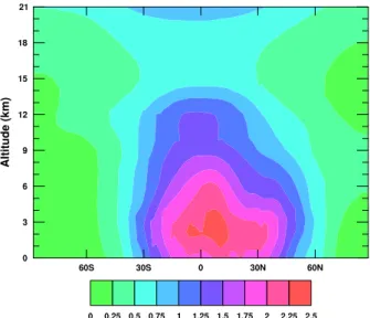
Fig. 2. Zonal Average MATCH OH concentration (molecules cm−3).
condition, but that the annually varying OH with annually repeating dynamics was most similar to the fully interannual run, showing that deduced emissions are more sensitive to OH than to transport. It is not clear however to what extent the OH fields are influenced by the interannually varying me-teorology used in the initial run.
Their treatment of the 1991–1992 anomaly is noteworthy. They mention the decreased growth rate in 1992 along with possible mechanisms, but not the increased growth rate in 1991, seen in Fig. 1 and discussed in the literature as men-tioned in Sect. 1. Their boundary condition (their Fig. 2) does not seem to include such a strong perturbation in the growth rate as observed in Fig. 1 or by others such as Dlugo-kencky et al. (1996) and Lowe et al. (1997). They did deduce a reduced source in 1992–1993 which they attributed to the effects of the Pinatubo eruption.
3 The CRC-MATCH CTM
The model used in this work is CRC-MATCH, the Coop-erative Research Centre (for Southern Hemisphere Meteo-rology) Model of Atmospheric Chemistry and Transport, a three dimensional chemical transport model developed at the CRC-SHM and based on the NCAR Community Climate Model (version 2)(Hack et al., 1994). It has previously been used for simulations of long-lived stratospheric trace species (Waugh et al., 1997) and tropospheric CO2(Law and Rayner,
1999), and was a part of the Transcom model intercompari-son project (Gurney et al., 2004). The model is run at a res-olution of 32 longitudes by 64 latitudes (11.25◦×2.81◦) with 44 levels in the vertical. The vertical coordinate system used is the hybrid pressure-sigma system. The vertical coordinates extend to the mesopause, at an altitude of about 70 km, with
Table 1. Nitrogen oxides sources (Tg(N)/yr).
Source Magnitude Industrial emissionsa 21 Biomass burningb 7.8 Soilsa 5.5 Lightningc 2 Total 36.3 aGEIA bGalanter et al. (2000) cGEIA, scaled
Table 2. Carbon monoxide sources (Tg(CO)/yr).
source Magnitude
Fossil fuel burninga 261
Industrial emissionsa 35 Anthropogenic NMHC oxidationa 235 Natural NMHC oxidationb 300 Biomass burningc 748 Oceansd 50 Total 1629 aEDGAR
bGEIA, Lawrence et al. (1999) cGalanter et al. (2000)
dBates et al. (1995), Lawrence et al. (1999)
increased vertical resolution in the planetary boundary layer and the tropopause. The model uses the semi-Lagrangian advection scheme of Williamson and Rasch (1989). To con-serve mass, a mass fixer is also used. Vertical diffusion is from Kiehl et al. (1998) and moist convection is from Hack (1994), which only allows tracer mass to be exchanged be-tween adjacent model layers, and so does not represent deep convection very well. This is more of a problem for species with lifetimes comparable to the timescales of deep convec-tion (such as NOx) than it is for CH4, although it could
po-tentially influence the inverse result through effects on the chemical sink of CH4due to the OH radical. Section 4
ex-amines the OH radical in more detail. The distributions of species such as O3, NOxand CO are described in detail in
Butler (2003).
The chemical scheme is also described fully in Butler (2003). It includes “background” tropospheric reactions of the CH4-CO-O3-NOxsystem as well as “background”
strato-spheric reactions including catalytic O3 destruction cycles,
Table 3. Tropospheric OH averages (molecules cm−3) compared. Distribution Airmass weighted CH4reaction weighted
MATCH 1.14 1.37
SMATCH 1.28 1.41
The emissions of NOxand CO used in CRC-MATCH are
summarised in Tables 1 and 2 respectively. NOxemissions
from industry and soils are taken from the GEIA inventory (Graedel et al., 1993), as are emissions from lightning which are scaled to a global rate of 2 Tg(N)/yr after Lawrence et al. (1999) and distributed vertically according to Pickering et al. (1998). NOx emissions due to biomass burning are from
Galanter et al. (2000). Anthropogenic emissions of CO from industry and fossil fuel combustion are from the EDGAR in-ventory (Olivier et al., 1996), along with a source from the oxidation of anthropogenically emitted NMHC, which is pa-rameterised here as a direct release of CO due to the lack of reactions involving NMHC in CRC-MATCH. Also treated this way are emissions of natural NMHCs from the GEIA in-ventory, which are scaled to 300 Tg(CO)/yr after Lawrence et al. (1999). Oceanic emissions of CO follow the pattern of Bates et al. (1995) and are scaled after Lawrence et al. (1999). Biomass burning emissions of CO are from Galanter et al. (2000).
The NMHCs accounted for in this study are of both natural (e.g. isoprene and monoterpenes; Graedel et al., 1993) and anthropogenic origin (e.g. aromatic and unsaturated com-pounds as well as longer lived alkanes such as ethane; Olivier et al., 1996) generally have lifetimes in the atmosphere rang-ing from hours to several days. Accountrang-ing for these emis-sions as direct emisemis-sions of the longer lived CO will tend to delocalise their effect away from the source regions, so the OH fields calculated in this study can be expected to be higher over continents than they would have been if the NMHCs were included directly in the model (e.g. Houwel-ing et al., 1998).
CRC-MATCH is an “offline” chemical transport model, meaning that it uses archived dynamics data (e.g. wind, pressure, temperature, humidity, diffusion and convection) instead of calculating these quantities. CRC-MATCH is driven by an annual cycle of archived dynamics from the NCAR Middle Atmosphere Community Climate Model (ver-sion 2)(Boville, 1995), which are stored at a 6 hourly interval and interpolated to the model timestep of one hour. The use of annually repeating dynamics from a climate model rather than analysed winds means that the effect of interannual vari-ability in the transport can not be explored. The mass bal-ance inverse results of Law and Simmonds (1996) for CO2
were less sensitive to this than they were to the concentra-tion boundary condiconcentra-tion, and the results of Dentener et al.
Table 4. Percentage of CH4oxidised in various subdomains of the
atmosphere from the (a) MATCH and (b) Spivakovsky OH distribu-tions. The vertical lines represent latitudes of 30◦S, 0◦, and 30◦N. The horizontal lines represent pressure levels of 750 hPa, 500 hPa, 250 hPa and the climatological tropopause.
5.4 0.2 0.2 2.0 3.1 3.5 5.0 3.4 9.1 10.5 12.2 3.9 12.5 15.3 13.7 2.4 0.3 0.2 3.5 4.7 4.6 4.9 6.9 13.3 12.7 11.4 4.5 9.8 10.8 9.9 (a) MATCH OH (b) Spivakovsky OH
(2003a) for CH4 were more sensitive to interannual
varia-tions in OH than in the transport (see Sect. 2). However the forward modelling study of Warwick et al. (2002) has shown that interannual variability in transport can be important in effecting the interannual variability in the CH4growth rate.
Also concerning is the sensitivity to the GCM used to pro-duce the dynamics data noted by Law and Vohralik (2001) as described in Sect. 2. Since the CRC-MATCH CTM used in this study is only capable of using annually repeating dy-namics data from a single source, these sensitivities cannot be explored in this study, and are an important topic for fu-ture work.
4 Hydroxyl radical
The average CH4 lifetime due to destruction by OH in the
troposphere from this run is 7.86 years. The average CH4
lifetime due to all chemical destruction processes through the entire model domain is 8.68 years. This is consistent with the figure of 90% of CH4being destroyed by reaction with OH in
the troposphere, mentioned in Sect. 1. The definition of “tro-posphere” used in these calculations is taken from Lawrence et al. (2001), who themselves compare a number of OH dis-tributions. The tropospheric CH4 lifetime from a number
of different OH distributions calculated by their version of MATCH ranges between 7.79 and 10.25 years, while they report the tropospheric CH4lifetime from the Spivakovsky
et al. (2000) OH distribution as 8.23 years.
Comparing the MATCH OH distribution (shown in Fig. 2) with other distributions from the literature, we look at the tropospheric airmass-weighted average and the tropospheric CH4 reaction weighted average (Table 3). Interestingly,
the averages of the Spivakovsky OH regridded onto the MATCH grid are somewhat higher than the values reported by Lawrence et al. (2001), and also higher than the airmass-weighted average reported by Spivakovsky et al. (2000) themselves (albeit over a different tropospheric domain). It is suspected that the process of vertically interpolating the OH
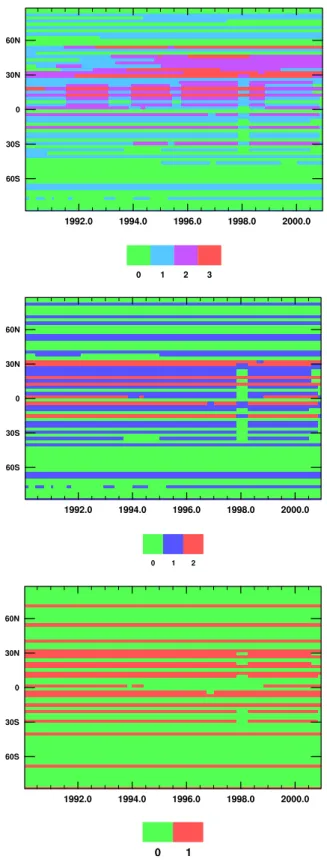
Fig. 3. The stations from the NOAA CMDL cooperative air sampling network used in this study, colors are explained in the text (Sect. 5.1).
number density between pressure levels used in this study is to blame for the discrepancy, because OH is conserved dur-ing the horizontal regridddur-ing process, but not durdur-ing the ver-tical regridding process. The CH4lifetime from the
regrid-ded Spivakovsky OH distribution is 7.66 years.
Lawrence et al. (2001) also analyse OH distributions by dividing the atmosphere into a number of subdomains and reporting the percentage of CH4oxidised in each. The same
analysis is performed here, and the results for the MATCH OH distribution are presented in Table 4a and for the Spi-vakovsky OH in Table 4b. The MATCH OH is very simi-lar to the OH from the three other versions of MATCH pre-sented by Lawrence et al. (2001). The percentage of CH4
ox-idised in each latitude band decreases with height, is larger in the tropics than the extratropics and larger in the NH than the SH. Comparing our version of the Spivakovsky OH with the analysis by Lawrence et al. (2001), there is more CH4
being oxidised in the tropics between 750 hPa and 500 hPa. The distributions used here also lead to proportionally more CH4 oxidation between 30 and 60 degrees north compared with Lawrence et al. (2001). There is no significant interan-nual variability in the distribution of CH4oxidation from the
MATCH OH field.
Another measure of OH concentration is the MCF (Methyl Chloroform, CH3CCl3) lifetime. The tropospheric MCF
life-time, calculated assuming a constant distribution of MCF in the troposphere, from the MATCH OH field is 4.81 years. This agrees well with the value of 4.6±0.3 years reported by Prinn et al. (1995) and Krol et al. (1998) for the period 1978– 1994. Lawrence et al. (2001) report MCF lifetimes in the range 4.66–6.16 years for their OH fields, and 4.95 years for
the Spivakovsky OH field. Using our analysis software and the Spivakovsky OH field regridded onto the MATCH grid, the MCF lifetime obtained is 4.63 years, which is only 94% of the lifetime reported by Lawrence et al. (2001). The dif-ference could be due to the regridding process as mentioned above.
5 Methane concentration boundary condition
5.1 Selection of data
All concentration boundary conditions used in this study are derived using monthly mean methane mixing ratio measure-ments from the NOAA CMDL cooperative air sampling net-work (Dlugokencky et al., 1994). The data is available from the internet via www.cmdl.noaa.gov. Sensitivity runs are performed using concentration boundary conditions derived from different subsets of the NOAA CMDL cooperative air sampling network in order to examine the sensitivity of the inverse results to temporal and physical gaps in the network, which were found by Law and Vohralik (2001) to be impor-tant (Sect. 2).
The three different subsets of the NOAA CMDL coopera-tive air sampling network used to construct the CH4
concen-tration boundary conditions used in this study are referred to hereafter as the “full”, “selected”, and “half” networks. The full network uses all of the available data from all measuring stations. The selected network is derived following Law and Vohralik (2001). Stations with more than 12 months of miss-ing data at the start or end of the period were not used. The half network case uses every second station (starting from
the South Pole) from the selected network case. The half network case is run to examine the sensitivity of the inverse result to geographical gaps in the measurement network.
Station locations are shown in Fig. 3, and explained in more detail in Butler (2003). Blue markers show the lo-cation of stations in the half network. Green markers refer to stations in the selected network which are not in the half network (i.e. the selected network consists of stations rep-resented by both blue and green markers). Likewise, red markers refer to stations in the full network which are not in the selected network (i.e. the full network consists of sta-tions represented by all markers). There are 68 stasta-tions in the full network, 38 in the selected network and 19 in the half network.
A graphical representation of the “density” of measure-ments from the full, selected and half networks is given in Fig. 4. This figure was produced by counting the number of measurements available for each month in each of the 64 lat-itude bands used by the CTM for each of the three networks. It shows the geographical coverage and length of the mea-surement record from the stations shown in Fig. 3. Compar-ing Figs. 4a, b and c the full network contains stations in the northern midlatitudes which came online in the mid 1990s. Based on Law and Vohralik (2001) this could be expected to influence the inverse results by introducing spurious in-terannual variability or trends into the boundary condition. All three figures show a substantial gap in the measurements around 1997–1998. This may also have some influence on the inverse result. These effects will be examined later in this study.
5.2 Construction of the boundary condition
Each station is assumed to be zonally representative, and a cubic smoothing spline is fitted through the data in sine lat-itude for each month to yield a zonal average CH4 mixing
ratio for each month from 1989–2000. Cubic smoothing splines have been shown to be particularly suitable for in-terpolating irregularly spaced atmospheric constituent data (Enting, 1987). The assumption that each station is zon-ally representative is not ideal, as stations at similar latitudes which are otherwise far apart can measure different mixing ratios (Law, 1999). It is possible to account for longitudinal variations in trace gas mixing ratios by using the measure-ments to adjust a previously calculated distribution of trace gas (Law, 1999), but this requires “a priori” knowledge of the sources of that trace gas.
Figure 5 shows the station data and smoothing splines for the three networks in February of 1990 and 1998 (the color scheme used is the same as for Fig. 3). The new stations measure higher mixing ratios than the stations which oper-ated continuously through the 1990s, and these new measure-ments lead to higher mixing ratio values in the smoothing spline for the half network. This could be expected to lead to an increasing trend in diagnosed emissions from the mass
Fig. 4. The station density (number of stations in each model lati-tude band) from the three networks. (a) The full network. (b) The selected network. (c) The half network.
Fig. 5. Station data (markers) and smoothing splines (lines) for the three networks (colors the same as for Fig. 3) in February 1990 and February 1998. (a) February 1990; (b) February 1998.
balance inverse procedure for the full network case. It may be that the extra measurements from the new stations in the northern midlatitudes provide a more zonally representative concentration boundary condition, but the fact that these sta-tions were not measuring during the early 1990s means that any increasing trend observed in these latitudes may not be real.
The effect of the gap in the measurement record for sta-tions in low southern latitudes observed in Fig. 4 can also be seen by comparing Figs. 5a and b. The absence of mea-surements between about 15◦–30◦S in 1998 leads to lower mixing ratio values in the smoothing spline around those lat-itudes in 1998 compared with 1990. This could be expected to lead to lower diagnosed emissions anomalies for those lat-itudes in 1998 compared with 1990.
The concentration boundary condition for the CTM is con-structed by appending all smoothing splines together in time to produce a latitude/time distribution of CH4surface mixing
Fig. 6. The CH4concentration boundary condition (ppb).
ratio. Figure 6 shows the resulting boundary condition cal-culated from the full network. Data were extrapolated back-wards one year in time (assuming a linear trend) so that 1988 and 1989 can be used as spinup years for the model. The boundary conditions derived from the selected and half mea-surement networks both appear very similar to the bound-ary condition derived from the full network (Fig. 6). All boundary conditions are dominated by the long term trend and seasonal cycle of CH4mixing ratio. The anomalies in
the concentration boundary conditions from the full and se-lected networks, calculated by removing the long term trend and seasonal cycles are presented in Figs. 14 and 15 where they are compared with the anomalies in the diagnosed fluxes from the mass balance inverse model runs.
From Fig. 3 one notices that there are numerous sites con-tributing measurements in the Pacific Ocean. This has the ef-fect of making the boundary condition more representative of the Pacific than of other sites at similar latitudes, especially in the Southern Hemisphere where most of the measurements that make up the boundary condition come from the Pacific. This effect can be seen by comparing the CH4timeseries at
5◦S in the Pacific Ocean with the timeseries from Ascension
Island which is located at 7◦S in the Atlantic Ocean (Fig. 7). In the Pacific, the boundary condition agrees quite well with the shipboard measurements, but is actually out of phase with the measurements from Ascension Island. This is not ideal but it is best to have a boundary condition which represents the largest possible area. See Butler (2003) for a more de-tailed comparison of the concentration boundary condition with observed mixing ratios.
6 Diagnosed CH4fluxes
Table 5 presents a summary of the specifications in each of the model runs. The average CH4sources from all five runs
Fig. 7. CH4 mixing ratio timeseries (ppb) at 5◦S in the Pacific
Ocean and at Ascension Island: observations (solid line) and bound-ary condition (dashed line). (a) 5◦S in the Pacific Ocean; (b) As-cension Island.
are within the range of 569–573 Tg/yr, which is well within the uncertainty range given by Houweling et al. (1999). This is despite the differing treatments of CH4 oxidation used
in these runs, and the different measurement networks used to construct the boundary condition. The diagnosed CH4
emissions fall within such a small range due to the similar CH4-reaction weighted averages of the OH distributions used
(Sect. 4), and the fact that the source and sink of CH4are
ap-proximately in balance.
6.1 Latitudinal structure
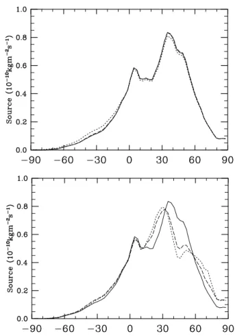
Figure 8a shows the zonal average of the deduced CH4fluxes
from the three inverse runs. The zonal distribution of fluxes from all three runs is virtually identical, and corresponds well with the zonal structure of the previous mass balance inverse studies of Saeki et al. (1998) and Law and Vohralik (2001). Figure 8b shows the sensitivity of the latitudinal structure of fluxes to the measurement network used to construct the
Fig. 8. Zonal average CH4fluxes (10−10kgm−2s−1): Sensitivity
to hydroxyl fields and choice of network. (a) The full chemistry (solid line), MATCH OH (dashed line) and Spivakovsky OH (dot-ted line) runs; (b) the Full Network (solid line), Selec(dot-ted Network (dashed line) and Half Network (dotted line) runs.
Table 5. Overview of all simulations performed.
Run Name Full Chemistry? Which Network?
Control yes full
MATCH OH no full
Spivakovsky OH no full
Selected no selected
Half no half
boundary condition. The fluxes are much more sensitive to the network than they are to the OH field used. The shift in the northern midlatitude emissions maximum seen in Fig. 8b is due to the effect of extra measurement stations coming on-line in the full network during the 1990s, as seen in Fig. 4a.
The structure of the sources from Fig. 8 also corresponds well with the methane sources as described in Sect. 1, and synthesis inverse studies such as Fung et al. (1991). The large peak in the northern midlatitudes corresponds with the
Fig. 9. Seasonal cycle of CH4fluxes from the full, selected, and half network runs (kg m−2s−1). Note the use of different scales. (a) The full network. (b) The selected network. (c) The half network.
anthropogenic emissions associated with fossil fuel produc-tion and use, as well as emissions from domestic ruminants and landfills. There is also a peak in the tropics which corre-sponds with the location of emissions from tropical wetlands and biomass burning. The latitudes between the two peaks correspond with the location of emissions from rice cultiva-tion. The absence of substantial emissions from the southern hemisphere corresponds with the mostly oceanic character of this hemisphere and hence the lack of significant sources of CH4. Considering the different techniques used in
construct-ing the concentration boundary condition and the different treatments of the chemical sink in all of these simulations, the degree of agreement between the studies on the basic lat-itudinal structure of the diagnosed CH4flux indicates that the
method is quite robust at describing this aspect of the global CH4budget.
6.2 Seasonal cycle
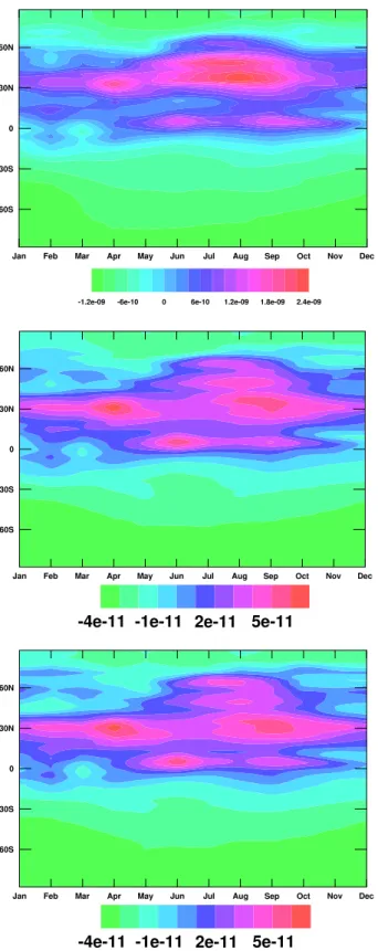
Figure 9 shows the climatological seasonal cycle of CH4
fluxes from runs performed with the three networks, obtained by averaging the flux from each month. Note that different scales are used in Fig. 9. The most striking feature of Fig. 9a is the large peak in the flux in northern midlatitudes between about June–September, which corresponds with the north-ern midlatitude peak seen in Fig. 8. The summer timing of this peak corresponds well with the timing of emissions from rice cultivation and boreal wetlands, although it is located in between the latitudes at which these sources would be ex-pected. There is also another distinct peak in the seasonal cycle of the deduced flux at 30◦N in April. None of the CH
4
sources listed in Sect. 1 can account for this diagnosed sea-sonal variability in the CH4flux. As mentioned in Sect. 1 the
northern midlatitude sources are generally assumed to have no seasonal variation.
Figures 9b and c are more similar to each other than ei-ther is to Fig. 9a, showing that the deduced seasonal cycle of fluxes is more sensitive to the addition of new stations into the network than it is to the size of the network. The new midlatitude stations coming online can be seen by comparing Figs. 5a and b. The fixed network (selected and half network) cases also produce a seasonal cycle of fluxes which is more consistent with the CH4 sources discussed in Sect. 1. The
midlatitude source shows less seasonal variation in the fixed network runs, and there is a more distinct peak from boreal wetlands.
All network cases show a seasonal peak in the flux from the northern tropics between June–October, which corre-sponds with seasonal emissions from low northern hemi-sphere wetlands. There are no distinct signatures of emis-sions from low southern hemisphere wetlands or biomass burning in either hemisphere in this climatological seasonal cycle of fluxes. The timing of these tropical sources was dis-cussed in Sect. 1.
Fig. 10. The year to year global-scale growth rate (solid line, left scale), deduced source (dashed line, right scale) and chemical sink (dotted line, right scale) in Tg/yr from the full-chemistry inverse run.
6.3 Interannual variability
Figure 10 shows the year to year global CH4 flux deduced
from the decadal inverse run with full chemistry, as well as the chemical sink from all reactions which remove CH4.
Also shown is the global growth rate, calculated from the sur-face mixing ratio trend which was previously shown in Fig. 1 by converting the volume mixing ratio to a mass mixing ratio and multiplying by the mass of the atmosphere. It appears that the diagnosed flux is being driven by the concentration boundary condition, which is what one would expect given that the boundary condition is the only part of the run with any interannual variability. The chemical sink shows a grad-ual increase with time because the CH4sink is proportional
to the concentration of CH4itself.
All the events mentioned in Sect. 1 are present in Fig. 10, namely the peaks in 1991, 1994, 1998, and the low growth event in 1992. Both Saeki et al. (1998) and Law and Vohralik (2001) also diagnose a large increase in the CH4flux in 1991
to account for the large increase observed in their boundary condition, and a decrease in the flux in 1992 corresponding to the decreased trend. Dentener et al. (2003a), whose bound-ary condition did not include such an increase in the trend in 1991, did not diagnose a large source, but they did diagnose a reduced source in 1992. This shows again that the forcing supplied by the concentration boundary condition can have a large effect on the fluxes diagnosed by the mass balance inverse method.
The high growth event in 1998 is interesting as it appears to be different from the events in 1991 and 1994. In the two earlier events there appears to be a close correspondence be-tween the peaks in the growth rate and the flux, but in 1998 the peak in the flux is less pronounced and broader than the peak in the growth rate. The differences between the 1997–
Fig. 11. The global-scale growth rate (solid line), deduced source from the full chemistry run (dashed line), seasonally repeating OH run with MATCH OH (dotted line) and seasonally repeating OH run with Spivakovsky OH (dashed-dotted line), in Tg/yr.
1998 event and the other events will be explored further in Sect. 7.
Figure 11 compares the global CH4 flux deduced from
the inverse runs with seasonally repeating OH with the flux deduced from the full chemistry run previously shown in Fig. 10. The two seasonally repeating OH runs are again more similar to each other than to the full chemistry run, from which they diverge over time, showing that the methane-hydroxyl feedback becomes more important over longer timescales. The difference in the annual flux of CH4 at the
end of the model run is only 6 Tg, or about 1% of the annual CH4flux. These differences are not important for this study
as results are generally presented as the interannual variabil-ity of anomalies, from which the mean source and long term trend has been subtracted.
Something else to note about Fig. 11 is the similarity of the interannual variability of the full chemistry and season-ally repeating OH runs. These similarities should not be in-terpreted as showing that interannual variability in the chem-istry is not important for CH4inversions, as there was no
in-terannual variability in any of the inputs to the model which could cause significant interannual variability in the OH con-centrations. The only source of interannual variability in the run was the CH4 boundary condition, which is driving the
interannual variability in the diagnosed CH4flux.
As seen in Fig. 10 the interannual changes in the CH4
mix-ing ratio do not cause significant interannual changes in the size of the CH4sink because they occur on timescales
signif-icantly shorter than the CH4lifetime. Interannual variability
in the chemical sink will be introduced in future work with an optical depth perturbation corresponding to an injection of aerosols into the stratosphere from the eruption of Mount Pinatubo, and an inverse run performed with a concentration
Fig. 12. The deduced source from the full network run (solid line), the selected network run (dashed line) and half network run (dotted line), in Tg/yr.
boundary condition for CO, which due to its much shorter lifetime than CH4has more of an influence on OH
concen-trations.
Figure 12 compares the CH4 flux deduced from inverse
runs with the boundary conditions from different measure-ment networks performed with annually repeating MATCH OH. Comparing Fig. 12 with Figs. 11 and 10, one sees that the inverse result is more sensitive to the choice of measure-ment network than to the representation of the CH4sink. The
two cases run with a relatively constant network (the selected and half network cases) are more similar to each other than to the full network case. This is due to the addition of spuri-ous interannual variability into the boundary condition when new stations come online, as described by Law and Vohralik (2001). Interestingly, the cases run with constant networks appear to be diagnosing a more pronounced peak in the flux in 1998 than the case run with the full network, which as commented on earlier produces a peak in the flux in 1998 which does not match the peak in the 1998 growth rate as well as it does for other years. This is despite the growth rate being calculated from the full network.
7 Anomalous interannual variability
7.1 Global scale
Figure 13 shows the sensitivity of the interannual variability of flux anomalies to the measurement network used to con-struct the boundary condition. We have plotted a 5 month running average of the monthly anomalies obtained by sub-tracting the global trend and the seasonal cycle at each grid point. The annually repeating MATCH OH was used in these runs due to the insensitivity of the interannual vari-ability of the anomalies to the OH field used (Fig. 11). All
Fig. 13. The flux anomaly (Tg/yr, 5 month running average) from the repeating OH inverse runs with the full network (solid line) with the selected network (dashed line), and with the half network (dot-ted line).
three flux anomaly curves from Fig. 13 show very similar structure, with the major differences being in the magnitude of the variability, which is consistent with Law and Vohra-lik (2001). The two cases run with constant networks show a more pronounced peak in the flux in 1998 than the case run with the full network, making them more consistent with Dlugokencky et al. (1998).
7.2 Latitudinal structure
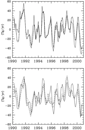
We now examine the latitudinal variability in the fluxes and explore how that variability is influenced by the boundary condition. Figure 14a shows the anomaly in the concentra-tion boundary condiconcentra-tion from the full network. This is calcu-lated by subtracting the climatological seasonal cycle and a linear fit to the long term trend from the concentration bound-ary condition shown in Fig. 6. Figure 15a is calculated simi-larly from the selected network boundary condition. Note the use of a different scale compared with Fig. 14a. Figure 14b
Fig. 14. The anomalies in the concentration boundary condition and diagnosed flux from the control run. (a) The concentration bound-ary condition anomaly (ppb). (b) The flux anomaly (kg m−2s−1).
shows the anomaly in the flux of CH4from the control run.
The anomaly is calculated by subtracting the climatological seasonal cycle of fluxes (Fig. 9) and a linear fit to the long term trend from the fluxes. Figure 15b is calculated similarly from the selected network model run. Note the use of a dif-ferent scale compared with Fig. 14b. The three events from Figs. 10 and 13 are all present in Figs. 14 and 15. Results for the half network case (not shown) are again very similar to the selected network case.
In general, mixing ratio anomalies are associated with flux anomalies. For example, the positive mixing ratio anoma-lies in low latitudes in 1991 are associated with positive flux anomalies. This is due to the mass balance inverse procedure supplying a flux to account for the increased mixing ratio. Not all changes in the mixing ratio anomaly in Figs. 14a and 15a can be directly related to respective flux anomalies in Figs. 14b and 15b however. For example there is a positive
Fig. 15. The anomalies in the concentration boundary condition and diagnosed flux from the selected network run. (a) The concen-tration boundary condition anomaly (ppb). (b) The flux anomaly (kg m−2s−1).
mixing ratio anomaly observed in high southern latitudes in 1992, with no corresponding flux anomaly. This is probably due to atmospheric transport of the CH4emissions
associ-ated with the tropical flux anomaly in 1991. This highlights the danger of simply diagnosing flux anomalies directly from growth rate anomalies: those growth rate anomalies may be due to atmospheric transport of a remote flux anomaly. This result is highly encouraging for our admittedly simple inverse technique. We did not specify, “a priori”, that there must not be a flux anomaly in high southern latitudes even though we knew this to be implausible. The inverse procedure correctly diagnosed the flux anomaly as occurring elsewhere.
Figure 16 shows the interannual variability of the flux anomalies from the four semi hemispheres from the three different network cases (note the different scales on each graph). As seen in Fig. 14b, the variability in high southern
(a) (b)
(c) (d)
Fig. 16. The CH4flux anomaly (Tg/yr) from the four semi-hemispheres for the full network (solid line), selected network (dashed line) and half network (dotted line) model runs. Note the use of different scales for each semi hemisphere. (a) 90◦–30◦S; (b) 30◦S–0◦. (c) 0◦–30◦N; (d) 30◦–90◦N.
latitudes is quite small. This is also apparent in Fig. 16a, and is consistent with the lack of any significant sources or sinks of CH4in these latitudes. Figure 16c (d) shows a
decreas-ing (increasdecreas-ing) trend in the low northern hemisphere (high northern hemisphere) which is not seen in the fixed network cases. These emissions trends can also be seen in in Fig. 14b and are likely to be caused by the addition of new stations into the network.
The differences between the fluxes from runs performed with boundary conditions derived from different measure-ment networks is greater at the semi hemispheric scale than at the global scale (compare Fig. 16 with Fig. 13). Again, however, the selected and half network cases are more sim-ilar to each other than to the full network case. This is inconsistent with the observation by Law and Vohralik (2001), whose smaller network did not diagnose regional (semi hemispheric) flux anomalies as well as their selected network. Their selected network consisted of 20 measuring stations while their half network consisted of 10. As
men-tioned in Sect. 5.1, our selected network has 38 stations and our half network 19. This suggests that a network with a size of about 20 stations is adequate for resolving the interannual variability of CH4 flux anomalies on the semi hemispheric
scale.
8 The major growth events in the 1990s
In the following sections, the major growth events mentioned in Sect. 1, and referred to briefly above are examined in more detail. The flux anomalies from the runs performed with the different networks are integrated in time and space to allow further examination of the sensitivity of these results to the boundary condition, and comparison of the events with the literature. For each latitude band examined below, the linear trend present in each network for that band is first subtracted from the timeseries before the integration is performed, al-lowing better comparison between networks with different long term trends, as was observed, for example, in Fig. 16c.
The removal of the long term trend from each band means that the sum of the flux anomalies from each semi hemi-sphere is not always equal to the global flux anomaly.
Quantitative comparison of the anomalies presented here with those presented in other studies is difficult due to dif-fering methods of calculating anomalies. For example, if the anomalies are created with a low-pass filter (e.g. Dlu-gokencky et al., 1998) then the frequency cut-offs will affect the results. Similarly, choices of the averaging period for the running means used in this study will affect the results.
8.1 Flux anomalies in 1991
Table 6a shows the integrated flux anomalies for the globe and the four semi hemispheres for 1991 in Tg for each of the three networks. The selected and half networks show very similar global flux anomalies, while the full network shows a global flux anomaly which is about 7 Tg larger, and a flux anomaly from the 0◦–30◦N region which is 10 Tg larger than the other networks. This is consistent with the suggestion by Law and Vohralik (2001) that measuring stations which came online around the time of the Mount Pinatubo eruption may have artificially inflated the measured global mixing ratio in-crease around this time. These new stations coming online can be seen in Fig. 4a. The use of a fixed measurement net-work removes this influence (Figs. 4a and b).
As mentioned in Sect. 1, a contributing factor to the large CH4 growth observed in 1991 may have been an
anoma-lously large source from biomass burning in the Amazon. Ta-ble 6a shows a consistent positive flux anomaly of 7–10 Tg in the 0◦–30◦S region across all networks, indicating that this anomaly is a robust feature of the inversion. This region in-cludes the Amazon, so the results here are consistent with increased biomass burning there, but since the flux anoma-lies are zonal averages, the results may be affected by flux anomalies elsewhere in the semi hemisphere. Interestingly, Table 6a shows an anomalous emission of 7 Tg deduced from both fixed networks in the 30◦–90◦N region which is not
de-duced from the full network.
In Sect. 1 we also mentioned a reduction in the CH4sink
resulting from the eruption of Mount Pinatubo as another suggested explanation of the mixing ratio increase observed in 1991. Since the model runs presented here do not include any such reduction in the sink it is possible that the model is responding erroneously with increased sources. The effect of the eruption on the deduced sources will be explored in future work.
Saeki et al. (1998) also noticed an increase in the global CH4 flux during 1991, but their increase was observed in
the 30◦N–90◦N latitude band. They actually diagnose a de-crease in the low latitude flux in 1991. Unfortunately they only report year to year changes in the flux, so it is not clear how their flux anomaly evolved during 1991. Law and Vohralik (2001) diagnose the increased flux in 1991 as com-ing entirely from the 15◦S–15◦N latitude band, with a
de-Table 6. Integrated global and semi-hemispheric flux anomalies (Tg) for (a) 1991 (b) 1992 (c) March 1994–February 1995 (d) September 1997–August 1998 (e) 1998.
Region Full Selected Half
Globe 27 20 19 30◦–90◦S 3 2 1 0◦–30◦S 10 8 7 0◦–30◦N 11 1 1 30◦–90◦N 1 7 7 (a) 1991
Region Full Selected Half
Globe −19 −23 −23 30◦–90◦S 0 1 0 0◦–30◦S −12 −12 −10 0◦–30◦N −4 −6 −6 30◦–90◦N −7 −7 −7 (b) 1992
Region Full Selected Half
Globe 8 6 9 30◦–90◦S −2 −2 0 0◦–30◦S −3 2 0 0◦–30◦N 16 12 14 30◦–90◦N −4 −6 −5 (c) March 1994–February 1995
Region Full Selected Half
Globe 11 18 19 30◦–90◦S −1 1 0 0◦–30◦S −7 −6 −8 0◦–30◦N 23 19 29 30◦–90◦N −2 5 −8 (d) September 1997–August 1998
Region Full Selected Half
Globe 4 21 21 30◦–90◦S 1 2 1 0◦–30◦S −2 −2 −5 0◦–30◦N −2 14 21 30◦–90◦N 8 8 5 (e) 1998
crease in the flux from the 15◦N–50◦N band. Dentener et al. (2003a) do not diagnose an increased flux in 1991 at all. The differences between Saeki et al. (1998), Law and Vohralik (2001), Dentener et al. (2003a) and this study would appear to be due to the differing methods of constructing the con-centration boundary condition, which has been seen above to have a large effect on the inverse results.
8.2 Flux anomalies in 1992
Table 6b shows the integrated flux anomalies for the globe and the four semi hemispheres for 1992 in Tg for each of the three networks. The results for all regions in Table 6b are consistent across all three networks, showing that the inverse procedure is not particularly sensitive to the choice of net-work during 1992. Comparison of Figs. 4a and b shows that the full network has gaps in the measurement record north of 30◦N during 1992, but these gaps do not appear to be af-fecting the deduced fluxes from this region. The results here are reasonably in accord with the suggestion by Lowe et al. (1997) that the reduced growth observed in 1992 can be ex-plained by an imbalance between sources and sinks of 20 Tg. As mentioned in Sect. 1 reduced biomass burning in the Amazon is a hypothesised mechanism for the low growth ob-served in 1992. The results from all networks in Table 6b for the region 0◦–30◦S show an anomalously low flux, although it is short of the 20 Tg suggested by Lowe et al. (1997). Both the 0◦–30◦N and 30◦–90◦N regions also show nega-tive emissions anomalies.
Walter et al. (2001) proposed anomalously low emissions from boreal wetlands to explain the low growth observed in 1992. Boreal wetland emissions are concentrated between 45◦–75◦N (Fung et al., 1991), and all three network cases show a negative emissions anomaly of 4–6 Tg between these latitudes in 1992, which is consistent with a negative emis-sions anomaly from boreal wetlands. Other sources between 45◦N and 75◦N are sources associated with fossil fuel pro-duction and use, domestic ruminant animals, landfills and termites (Fung et al., 1991). van Aardenne et al. (2001) re-port long term increasing trends in the fossil fuel and to a lesser extent the landfill source up to 1990, but it is unclear how much interannual variability these sources show.
As discussed in Sect. 1, there may have also been a change in the atmospheric solar radiation budget during 1992 result-ing from the Mount Pinatubo eruption. The presence of scat-tering aerosols in the stratosphere (Dlugokencky et al., 1996) and stratospheric O3depletion (Bekki et al., 1994) may have
altered the OH concentration in the troposphere and thus changed the sink of CH4. Bekki et al. (1994) suggested that
the stratospheric O3depletion could account for up to half of
the observed decrease in the CH4growth rate in 1992, which
from Table 6b would translate to an increase in the global source of about 10 Tg. This should be considered an upper limit on the source increase due to the effects of stratospheric O3depletion, for the reasons discussed in Sect. 1. The effects
of the Mount Pinatubo eruption are not included in the con-trol run or the network sensitivity runs, but will be explored in future work.
8.3 Flux anomalies in 1994–1995
Table 6c shows the integrated flux anomalies for the globe and the four semi hemispheres between March 1994 and
February 1995 in Tg for each of the three networks. Lan-genfelds et al. (2002) suggested the CH4growth anomaly in
1994–1995 could be explained by a 12 month pulse of 26 Tg from biomass burning centred on August 1994.
The results from the three networks are again quite con-sistent, showing that the inverse results are not particularly sensitive to the choice of measurement network. Interest-ingly, the 1994–1995 event is different to the 1991 and 1992 events in that it appears to have a clear spatial structure, with positive emissions anomalies in the 0◦–30◦N region, with no positive emissions anomalies in any other semi hemisphere. This structure can also be seen in Fig. 14.
Neither the global flux anomaly of 6–9 Tg nor the flux anomaly of 12–16 Tg from 0◦–30◦N seen in Table 6c are
consistent with the 26 Tg of anomalous emissions suggested by Langenfelds et al. (2002) to explain the 1994–1995 event. This inconsistency may not be due to the different measure-ment networks used by Langenfelds et al. (2002) and this study, as the half network with its 12 measuring stations and the 10 station network of Langenfelds et al. (2002) have a similar size, and Law and Vohralik (2001) found that such small fixed networks are capable of resolving similar global CH4mixing ratio anomalies to larger fixed networks such as
the selected network used here. Perhaps the different net-work geometry used by Langenfelds et al. (2002) (including use of vertical profile data above Cape Grim) could be con-tributing extra information to their study which is leading to the different emissions estimates between that study and this one. Cunnold et al. (2002), as evidenced from their Fig. 5 do not seem to diagnose any significant emissions anomaly in 1994–1995 either. They do not use vertical profile data. Law and Vohralik (2001) did notice a positive emissions anomaly in 1994–5, occurring between 15◦S–15◦N, but do not report an integrated flux for the period examined here. They do not use vertical profile data either. The results of Law and Vohra-lik (2001) for the 1994–1995 event show more sensitivity to the source of the dynamics data used to drive their CTM than the other events do. Perhaps anomalous CH4mixing ratios
observed in 1994–1995 are related to anomalous transport around that time. The differences in the treatment of trans-port between Langenfelds et al. (2002) and this study (single box model compared with 3-D CTM) may possibly be con-tributing to the differences observed here.
8.4 Flux anomalies in 1997–1998
Langenfelds et al. (2002) suggested the CH4growth anomaly
in 1997–1998 could be explained by a 12 month pulse of 33 Tg from biomass burning centred on February 1998. Ta-ble 6d shows the integrated flux anomalies for the globe and the four semi hemispheres between September 1997 and Au-gust 1998 in Tg for each of the three networks.
The results from the three networks show some large dif-ferences. The two fixed size networks show similar global flux anomalies compared with the full network, but show
large differences between the two in both northern semi hemispheres. It was noted in Sect. 5 that there were many gaps in the measurement record around 1997–1998. These gaps affect all three networks, as seen in Fig. 4, so for the 1997–1998 event, none of the three networks used here can be regarded as “fixed”. As noted by Law and Vohralik (2001), and seen here for the 1991 event in Sect. 8.1, a chang-ing network can introduce spurious variability into the results of an inversion, so the results for this event for all networks should be treated with suspicion.
None of the networks in Table 6d produce a global flux anomaly which is close to the 33 Tg estimated by Langen-felds et al. (2002) obtained using a network with no gaps. Interestingly, all three networks agree on a negative flux anomaly of 6–8 Tg for the 0◦–30◦S semi hemisphere. Closer examination of Fig. 4 reveals that the gap in the measurement record during this period for the southern hemisphere spans a particularly large latitude range. Figure 16b also shows an extremely pronounced dip in the flux anomaly for the 0◦– 30◦S region. It appears that the lack of measurements in the low southern hemisphere may be causing the smoothing spline procedure which constructs the boundary condition to assign measurements more appropriate to the high southern hemisphere to the low southern hemisphere. This was seen in Fig. 5b, and examination of Figs. 14 and 15 would appear to confirm this. It is not clear why there is such a large spread of flux anomalies between the networks in the 30◦–90◦N re-gion when there are no gaps in any of the networks north of about 30◦N. Given these concerns, it appears that all that can be said about the 1997–1998 event based on the results shown here is that there was a positive global flux anomaly which was primarily located in the 0◦–30◦N region.
Using a satellite measurements of burnt areas, Levine (1999) estimated a lower limit of 3 Tg(CH4) of emissions
(with an uncertainty of 50%) from Kalimantan and Sumatra during the 8 month period from August 1997 to March 1998. The full, selected and half network cases diagnose emissions anomalies of 11, 5, and 6 Tg respectively for this 8 month period. The selected and half network cases are more con-sistent with Levine (1999) than the full network case, which is interesting, given that the half network does not appear to be affected by the gaps in the measurements from this re-gion as the other two networks are (Fig. 4). It should also be noted that these flux anomalies are zonal averages and may be affected by emissions from elsewhere around that latitude band.
8.5 Flux anomalies in 1998
The detrended global and semi hemispheric flux anomalies for the calendar year 1998 are also presented here (Table 6e) to allow comparison with the study of Dlugokencky et al. (2001), who suggested that the growth observed in 1998 cor-responded to an anomalous increase in the imbalance be-tween sources and sinks of 24 Tg. They used a wetland
model to estimate anomalous emissions from the 0◦–30◦S
and 30◦–90◦N semi hemispheres of about 12 Tg each, but
acknowledge that these model derived wetland emissions should be treated with caution. Dlugokencky et al. (2001) also pointed out that there were also an estimated 6 Tg re-leased from boreal biomass burning in 1998, and noted a qualitative agreement between the location of these emis-sions anomalies and the observed growth in CH4mixing
ra-tio. The direct comparison between the physical locations of the observed mixing ratio increases and the emissions anomalies from the wetland model and biomass burning es-timates used by Dlugokencky et al. (2001) is different from the inverse modelling methodology employed here, as it does not include the effects of atmospheric transport.
As seen in Fig. 4 there were substantial gaps in the mea-surement record around this time. Similarly to the flux anomalies for the 1997–1998 event shown in Table 6d, the flux anomalies from Table 6e show a high sensitivity to the choice of measurement network, again suggesting that the gaps in the measurements may be influencing the deduced fluxes.
The gaps in the measurements, and the differing method-ologies make comparison of the results presented in Table 6e and by Dlugokencky et al. (2001) difficult. The anomalous global flux from both the selected and half network cases is 21 Tg, which is similar to the anomalous global imbal-ance between sources and sinks of 24 Tg, as noted by Dlugo-kencky et al. (2001), but the distribution of this flux anomaly seems poorly constrained by the available measurements. The selected and half networks in Table 6e are not as consis-tent with each other as they are for the 1992, and 1994–1995 events (Tables 6b and c), but as for the 1991 and 1997–1998 events (Tables 6a and d) they are more consistent with each other than with the full network.
The runs done with both networks seem to be suggesting that the growth in 1998 was primarily from the 0◦–30◦N re-gion, with a small contribution from the 30◦–90◦N region, and a weakly negative emissions anomaly from the 0◦–30◦S region. These flux anomalies are not close to either of the modelled wetland emissions anomalies from Dlugokencky et al. (2001), but they are consistent with about 6 Tg of emis-sions from boreal biomass burning, and perhaps some of the northern tropical biomass burning seen in Sect. 8.4 and noted by Langenfelds et al. (2002) which overlaps with this event by 7 months. Perhaps some of the growth observed by Dlu-gokencky et al. (2001) in the 0◦–30◦S and 30◦–90◦N regions may be due to transport of emissions from the 0◦–30◦N re-gion.
9 Conclusions
The inverse modelling approach used in this study is capable of resolving the global annual flux of CH4, its latitudinal