Arctic smoke ? record high air pollution levels in the European Arctic due to agricultural fires in Eastern Europe in spring 2006

HAL Id: hal-00296130

https://hal.archives-ouvertes.fr/hal-00296130

Submitted on 26 Jan 2007

HAL is a multi-disciplinary open access

archive for the deposit and dissemination of

sci-entific research documents, whether they are

pub-lished or not. The documents may come from

teaching and research institutions in France or

abroad, or from public or private research centers.

L’archive ouverte pluridisciplinaire HAL, est

destinée au dépôt et à la diffusion de documents

scientifiques de niveau recherche, publiés ou non,

émanant des établissements d’enseignement et de

recherche français ou étrangers, des laboratoires

publics ou privés.

European Arctic due to agricultural fires in Eastern

Europe in spring 2006

A. Stohl, T. Berg, J. F. Burkhart, A. M. Fj?raa, C. Forster, A. Herber, Ø.

Hov, C. Lunder, W. W. Mcmillan, S. Oltmans, et al.

To cite this version:

A. Stohl, T. Berg, J. F. Burkhart, A. M. Fj?raa, C. Forster, et al.. Arctic smoke ? record high air

pollution levels in the European Arctic due to agricultural fires in Eastern Europe in spring 2006.

Atmospheric Chemistry and Physics, European Geosciences Union, 2007, 7 (2), pp.511-534.

�hal-00296130�

www.atmos-chem-phys.net/7/511/2007/ © Author(s) 2007. This work is licensed under a Creative Commons License.

Chemistry

and Physics

Arctic smoke – record high air pollution levels in the European

Arctic due to agricultural fires in Eastern Europe in spring 2006

W. W. McMillan5, S. Oltmans6, M. Shiobara7, D. Simpson4, S. Solberg1, K. Stebel1, J. Str¨om8, K. Tørseth1, R. Treffeisen3, K. Virkkunen9,10, and K. E. Yttri1

1_{Norwegian Institute for Air Research, Kjeller, Norway} 2_{University of California, Merced, USA}

3_{Alfred Wegener Institute, Bremerhaven, Germany} 4_{Meteorological Institute, Oslo, Norway}

5_{University of Maryland, Baltimore, USA}

6_{Earth System Research Laboratory, NOAA, Boulder, USA} 7_{National Institute of Polar Research, Tokyo, Japan}

8_{Department of Applied Environmental Science, Stockholm University, Sweden} 9_{Arctic Centre, University of Lapland, Finland}

10_{Department of Chemistry, University of Oulu, Oulu, Finland}

*_{now at: Norwegian University of Science and Technology, Trondheim, Norway}

Received: 14 September 2006 – Published in Atmos. Chem. Phys. Discuss.: 5 October 2006 Revised: 8 January 2007 – Accepted: 19 January 2007 – Published: 26 January 2007

Abstract. In spring 2006, the European Arctic was

abnor-mally warm, setting new historical temperature records. Dur-ing this warm period, smoke from agricultural fires in East-ern Europe intruded into the European Arctic and caused the most severe air pollution episodes ever recorded there. This paper confirms that biomass burning (BB) was indeed the source of the observed air pollution, studies the transport of the smoke into the Arctic, and presents an overview of the observations taken during the episode. Fire detections from the MODIS instruments aboard the Aqua and Terra satel-lites were used to estimate the BB emissions. The FLEX-PART particle dispersion model was used to show that the smoke was transported to Spitsbergen and Iceland, which was confirmed by MODIS retrievals of the aerosol optical depth (AOD) and AIRS retrievals of carbon monoxide (CO) total columns. Concentrations of halocarbons, carbon diox-ide and CO, as well as levoglucosan and potassium, mea-sured at Zeppelin mountain near Ny ˚Alesund, were used to further corroborate the BB source of the smoke at Spitsber-gen. The ozone (O3) and CO concentrations were the highest

ever observed at the Zeppelin station, and gaseous elemental mercury was also elevated. A new O3record was also set at

a station on Iceland. The smoke was strongly absorbing – black carbon concentrations were the highest ever recorded

Correspondence to: A. Stohl

(ast@nilu.no)

at Zeppelin – and strongly perturbed the radiation transmis-sion in the atmosphere: aerosol optical depths were the high-est ever measured at Ny ˚Alesund. We furthermore discuss the aerosol chemical composition, obtained from filter sam-ples, as well as the aerosol size distribution during the smoke event. Photographs show that the snow at a glacier on Spits-bergen became discolored during the episode and, thus, the snow albedo was reduced. Samples of this polluted snow contained strongly elevated levels of potassium, sulphate, ni-trate and ammonium ions, thus relating the discoloration to the deposition of the smoke aerosols. This paper shows that, to date, BB has been underestimated as a source of aerosol and air pollution for the Arctic, relative to emissions from fossil fuel combustion. Given its significant impact on air quality over large spatial scales and on radiative processes, the practice of agricultural waste burning should be banned in the future.

1 Introduction

The European sector of the Arctic saw unprecedented warmth during the first months of the year 2006. At Ny ˚Alesund on the island of Spitsbergen in the Svalbard archipelago, the monthly mean temperatures from January to May were 10.7, 3.8, 1.4, 10.3, and 4.2◦C above the

corre--15 -10 -5 0 5 0401 0408 0415 0422 0429 0506 0513 0520 0527 Temperature (deg C) Date Temperature Normal temperature

Fig. 1. Time series of the 2-m air temperatures at Ny ˚Alesund on Spitsbergen measured at 00:00, 06:00, 12:00 and 18:00 UTC, from 1 April to 1 June 2006 (solid line). Shown for reference is the cli-matological mean temperature since 1969 for the same time period (dashed line).

sponding values averaged over the period since 1969 (Mete-orological Institute, 2006); the January, April and May val-ues were the highest ever recorded. Figure 1, a comparison between the temperatures measured at Ny ˚Alesund in April and May 2006 with the corresponding climate mean, shows that the entire two months were warmer than normal. Due to the abnormal warmth, the seas surrounding the Svalbard archipelago were almost completely free of closed ice at the end of April, for the first time in history. In contrast to the Arctic, the European continent saw a delayed onset of spring in 2006. Snow melt in large parts of Europe occurred only in April; even as late as 1 May, snow covered much of Scandi-navia.

Related to the abnormal warmth in the Arctic, record-high levels of air pollution were measured at the Zeppelin station near Ny ˚Alesund on Spitsbergen. It will be shown in this pa-per that they were caused by transport of smoke from agricul-tural fires in Eastern Europe. The most severe air pollution episodes happened on 27 April and during the first days of May 2006 when the concentrations of most measured air pol-lutants (aerosols, O3, etc.) exceeded the previously recorded

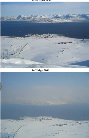
long-term maxima. Views from the Zeppelin station clearly showed the decrease in visibility from the pristine condi-tions on 26 April to when the smoke engulfed Svalbard on 2 May (Fig. 2). Iceland, where a new O3record was set at

the Storhofdi station, was also affected by the smoke plume.

2 Arctic air pollution

Because of its remoteness, the Arctic troposphere was long believed to be extremely clean but in the 1950s, pilots flying over the North American Arctic discovered a strange haze (Greenaway, 1950; Mitchell, 1957), which decreased

visi-Fig. 2. View from the Zeppelin station (a) under clear conditions on

26 April, and (b) during the smoke episode on 2 May 2006. Image courtesy of Ann-Christine Engvall.

bility significantly. The Arctic Haze, accompanied by high levels of gaseous air pollutants (e.g., hydrocarbons; Solberg et al., 1996), was observed regularly since then and is a re-sult of the special meteorological situation in the Arctic in winter and early spring (Shaw, 1995). Temperatures at the surface become extremely low, leading to a thermally very stable stratification with frequent and persistent occurrences of surface-based inversions (Bradley, 1992) that reduce tur-bulent exchange, hence dry deposition. The extreme dryness minimizes wet deposition, thus leading to very long aerosol lifetimes in the Arctic in winter and early spring. After po-lar sunrise, photochemical activity increases and can produce phenomena such as the depletion of O3and gaseous

elemen-tal mercury (GEM) (Lindberg et al., 2002).

Surfaces of constant potential temperature form closed domes over the Arctic, with minimum values in the Arctic boundary layer (Klonecki et al., 2003). This transport barrier isolates the Arctic lower troposphere from the rest of the at-mosphere. Meteorologists realized that in order to facilitate

isentropic transport, a pollution source region must have the same low potential temperatures as the Arctic Haze layers (Carlson, 1981; Iversen, 1984; Barrie, 1986). For gases and aerosols with lifetimes of a few weeks or less, this rules out most of the world’s high-emission regions as potential source regions because they are too warm, and leaves northern Eura-sia as the main source region for the Arctic Haze (Rahn, 1981; Barrie, 1986; Stohl, 2006). Transport from Eurasia is highly episodic and is often related to large-scale blocking events (Raatz and Shaw, 1984; Iversen and Joranger, 1985).

Boreal forest fires are another large episodic source of Arc-tic air pollutants, parArc-ticularly of black carbon (BC) (Lavou´e et al., 2000), which has important radiative effects in the Arc-tic, both in the atmosphere and if deposited on snow or ice (Hansen and Nazarenko, 2004). They occur in summer when wet and dry deposition are relatively efficient and the Arc-tic troposphere is generally cleaner than in winter. Never-theless, an aircraft campaign in Alaska frequently sampled aerosol plumes from Alaskan and maybe also Siberian for-est fires (Shipham et al., 1992), and a PhD thesis suggfor-ests that BC observations at Arctic sites are linked to boreal for-est fires (Lavou´e, 2000). Recently, Stohl et al. (2006) showed that severe forest fires burning in Alaska and Canada led to strong pan-Arctic increases in light absorbing aerosol con-centrations during the summer of 2004.

3 Observations

We present measurements mostly from the research station Zeppelin (11.9◦E, 78.9◦N, 478 m a.s.l.). The station is sit-uated in an unperturbed Arctic environment on a ridge of Zeppelin mountain on the western coast of Spitsbergen. Be-cause of the altitude difference and the generally stable atmo-spheric stratification, contamination from the nearby small settlement of Ny ˚Alesund (located near sea level) is minimal at Zeppelin.

Hourly O3 concentrations were recorded by

UV-absorption spectrometry (API 400A). GEM was measured using a Tekran gas phase mercury analyzer (model 2537A) as described in Berg et al. (2003). CO was measured us-ing a RGA3 analyzer (Trace Analytical) fitted with a mer-curic oxide reduction gas detector. Five ambient air mea-surements and one field standard were performed every 2 h. The field standards were referenced against a Scott-Marine Certificated standard and a calibration scale (Langenfelds et al., 1999; Francey et al., 1996).

Carbon dioxide (CO2) was measured using a

Non-dispersive Infrared Radiometer (NDIR), Li-COR model 7000. The radiometer was run in differential mode using a reference gas with a CO2content near the measured

concen-trations. Roughly every 2 h the radiometer was calibrated us-ing three different CO2concentrations spanning the expected

atmospheric concentration interval. Halocarbons were an-alyzed by gas chromatography/mass spectroscopy (Agilent,

5793N) at 4-hourly intervals. Substances from 2 l of air were preconcentrated on an automated adsorption-desorption sys-tem filled with three different adsorbents. This preconcen-tration unit was developed by the University of Bristol (Sim-monds et al., 1995) and has been in operation in the AGAGE network for several years (Prinn et al., 2000).

The particle size distributions were measured using a ferential Mobility Particle Sizer (DMPS) consisting of a Dif-ferential Mobility Analyser (Knutson and Whitby, 1975) and a TSI 3010 particle counter. The sheath flow is a closed-loop system (Jokinen and Makela, 1997). DMPS data from Zeppelin have been presented previously (Str¨om et al., 2003) and cover the size range from 13.5 to 700 nm diameter (bin limits).

Information on light absorbing particles was gathered with a custom-built particle soot absorption photometer (PSAP). In this instrument, light at 530 nm wavelength illuminates two 3 mm diameter spots on a single filter substrate, on one of which particles are collected from ambient air flushed through the filter, and the other kept clean as a reference. The change in light transmittance across the filter is mea-sured to derive the particle light absorption coefficient σap,

ignoring the influence of scattering particles. Conversion of

σap to BC concentrations requires the assumptions that all

the light absorption measured is from BC, and that all BC has the same light absorption efficiency. We convert σap values

to equivalent BC (EBC) mass concentrations using a value of 10 m2g−1, typical of aged BC aerosol (Bond et al., 2005).

Aerosol filter samples were collected for subsequent anal-ysis of the aerosols’ content of anions (Cl−, NO−₃, SO2−₄ ) and cations (Ca2+, Mg2+, K+, Na+, NH+₄) on a daily basis using an open face NILU filter holder, loaded with a 47 mm diameter Teflon filter (Zefluor 2 µm). The cations and an-ions were quantified by ion chromatography. While NO−₃ and NH+₄ are subject to both positive and negative biases, we only report the sum of particulate and gaseous phases for the two. For conditions typical for Norway, the particulate phase is the dominant fraction accounting for 80–90% of NO−₃ and approximately 90% of NH+₄. Aerosol samples were also col-lected on 8′′×10′′ cellulose filters (Whatman 41) according to a 2+2+3 days weekly sampling scheme, using a high vol-ume sampler with a 2.5 µm cut off. Using these samples, the aerosols’ content of levoglucosan was analyzed with high performance liquid chromatography combined with time-of-flight high-resolution mass spectrometry (HPLC/HRMS) as described by Dye and Yttri (2005). Finally, weekly aerosol samples were collected using a Leckel SEQ47/50 sampler loaded with prefired quartz fibre filters. The samples’ content of elemental carbon (EC) and organic carbon (OC) was quan-tified using the NIOSH 5040 thermo-optical method (Birch and Cary, 1996), which accounts for pyrolytically generated EC during the analysis.

At Ny ˚Alesund, daylight measurements of the spectral aerosol optical depth (AOD) were made with the automatic

sun photometer SP1A which uses the imaging method of Leiterer and Weller (1988). Seventeen channels cover the spectral range from 350 to 1065 nm with a full-width-half-maximum of 5 to 15 nm. The accuracy of the measured AOD is between 0.005 and 0.008. The measurement time is less than 5 s but the data presented here are hourly mean values. More details can be found in Herber et al. (2002).

A Micro-Pulse Lidar Network (MPLNET) instrument (Welton et al., 2001) is operated for the National Institute of Polar Research (Japan) at Ny ˚Alesund by the Alfred Wegener Institute for Polar and Marine Research, Germany, since 2002. The MPL uses a Nd/YLF laser, emitting laser light at a wavelength of 523.5 nm. Details regarding on-site main-tenance, calibration techniques, description of the algorithm used and data products are given in Campbell et al. (2002). We present the corrected normalized relative backscatter sig-nal, which corresponds to the raw signal counts from the MPL, processed to remove all instrument related parameters except the calibration constant. Since the molecular return gives rise to a range-corrected signal decrease of 50% be-tween ground and 5 km altitude due to the molecular den-sity decrease, we normalized the relative backscatter with the molecular return using a standard-atmospheric density pro-file. The data are stored at 1 minute time resolution and 30 m vertical resolution.

In addition to the measurements from Spitsbergen, we also present surface O3measurements from Storhofdi (20.34◦W,

63.29◦N, 127 m a.s.l.) on the southernmost tip of the island of Heimay in the Westman Islands, a group of small volcanic islands to the south of the principal island of Iceland. The preponderance of airflow is from off the Atlantic Ocean and there is only a small population center about 5 km north of the measurement site. Ozone measurements are made using a Thermo Environmental Instruments (TEI) model 49C an-alyzer, which has been regularly intercompared with a sec-ondary standard O3analyzer maintained by the NOAA Earth

System Research Laboratory, Global Monitoring Division. This secondary standard is calibrated against a standard ref-erence O3photometer maintained by the U.S. NIST.

For studying the transport and geographical extent of the aerosol pollution, we also used satellite measurements. To-tal column CO was retrieved from the Atmospheric InfraRed Sounder (AIRS) in orbit onboard NASA’s Aqua satellite. All AIRS retrievals for the given days were binned to a 1×1◦grid. The prelaunch AIRS CO retieval algorithm was employed using the AFGL standard CO profile as the first guess and the AIRS team retrieval algorithm PGE v4.0. Al-though AIRS CO retrievals are most sensitive to the mid-troposphere, the broad averaging kernel can be influenced by enhanced CO abundances near the boundary layer (McMil-lan et al., 2005, 20061).

1_{McMillan, W. W., Warner, J. X., McCourt Comer, M., Maddy,}

E., Chu, A., Sparling, L., Eloranta, E., Hoff, R., Sachse, G., Barnet, C., Razenkov, I., and Wolf, W.: AIRS views of transport from

10-The daily level 3 AOD data at a wavelength of 550 nm, retrieved with algorithm MOD08 D3 from the MODIS Terra Collection 4, were also used. A description and validation of these data can be found in Remer et al. (2005) and Ichoku et al. (2005). Their stated accuracy is ±(0.05+0.2×AOD) over land and ±(0.03+0.05×AOD) over ocean. Retrievals are not being made in cloudy areas, or in regions with a high surface albedo, e.g. over most of snow-covered Norway, and in ice-covered parts of the Arctic.

4 Biomass burning emissions

In April and May 2006, a large number of fires occurred in the Baltic countries, western Russia, Belarus, and the Ukraine. The fires were started by farmers who burned their fields before the start of the new growing season. This prac-tice is illegal in the European Union but is still widely used in Eastern Europe for advancing crop rotation and control-ling insects and disease. It is quite common that agricul-tural fires get out of control and devastate nearby forests or human property. According to newspaper reports (see http://www.baltictimes.com), the fires burned into the forests of the nature preserve Kuronian Spit in Lithuania and could be extinguished only after considerable efforts. Five people died in the fires in Latvia.

For estimating biomass burning (BB) emissions from these fires, we used active fire detections by the MODIS instruments onboard the Aqua and Terra satel-lites. These detections are based on MODIS Collection 4 data and the MOD14 and MYD14 algorithms (Giglio et al., 2003) (see http://maps.geog.umd.edu/products/MODIS Fire Users Guide 2.2.pdf). A number between 0 and 100 characterizes the confidence for every fire detection. We only used detections with a confidence level greater than 75. The algorithm uses data from pixels of about 1 km2size but the actual fire size is not known. Fires of 1000 m2or less can be detected under good observing conditions but even large fires can be obscured by clouds. Furthermore, detections can only be made at the time of the satellite overpasses and the number of detections also depends on the minimum confidence level requested. In the absence of better information, we assumed that every detection represents a burned area of 180 ha, based on a statistical analysis of MODIS fire detections with inde-pendent area burned data by Wotawa et al. (2006). This shall account both for the area burned by the detected fire itself and undetected fires in its vicinity on the same day.

Figure 3 shows the daily number of the detected fires in the region north of 40◦N and between 20 and 60◦E. More than 300 fires/day were detected from 25 April to 6 May 2006, with a peak of more than 800 detections on 2 May. This

23 July 2004 Alaskan/Canadian fires: Correlation of AIRS CO and MODIS AOD and comparison of AIRS CO retrievals with DC-8 in situ measurements during INTEX-NA/ICARTT, J. Geophys. Res., submitted, 2006.

0 200 400 600 800 1000 0401 0408 0415 0422 0429 0506 0513 0520 0527 0 0.2 0.4 0.6 0.8 1 1.2 1.4 1.6 1.8

Daily number of fire detections

Column CO (g/m2), Accumulated area burned (Mha)

Date Area burned Fire detections Column CO

Fig. 3. Time series of daily number of MODIS fire detections in the

region north of 40◦N and between 20◦E and 60◦E (black line) and estimated area burned in this region, accumulated from 1 April 2006 and assuming that 180 ha burned per detected fire (red line). Also shown are measurements of total column CO taken at Zvenigorod (blue symbols).

leads to an estimate of almost 2 million hectare burned in April and May 2006. The decrease in the number of fire de-tections on 28–30 April is likely not due to an actual decrease in fire activity but to the presence of clouds near 32◦E and 54◦N. In a crude attempt to account for the cloud effect on 28–30 April, we doubled the fire pixels in a small area to the northeast of the clouds and shifted these “shadow” pixels to the southwest into the cloud band. This increased the number of detections by about 40% on 28 and 29 April and 10% on 30 April. This correction was not applied to the data shown in Fig. 3 but was used for all subsequent calculations.

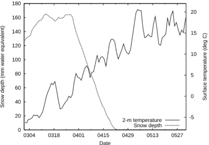
Figure 4 shows time series of the surface temperature and snow depth (shown as mm water equivalent), averaged over the region where most of the fires burned. There was a lot of snow on the ground until the end of March, which started melting in April. The fire frequency increased dra-matically on 21 April (see Fig. 3), after all the snow had disappeared. Korontzi et al. (2006) show that spring-time agricultural burning in Eastern Europe peaked in March in the year 2002 and in April in the years 2001 and 2003, whereas in all three years there was very little burning in May. In 2002, a smoke episode caused by agricultural fires in this region was observed in Finland already in the mid-dle of March (Niemi et al., 2004). In 2006, in contrast, farmers were forced to wait with the burning for the un-usually late snow melt, causing a strong emission pulse at the end of April/beginning of May (see Fig. 3) when fields were quickly prepared for the already delayed sowing. This is demonstrated also by the infrared spectroscopy measure-ments of total column CO made at Zvenigorod (36◦E, 55◦N; see Yurganov et al., 1995), which is located about 50 km west of Moscow and within the general burning region (symbols

0 20 40 60 80 100 120 140 160 180 0304 0318 0401 0415 0429 0513 0527 -5 0 5 10 15 20

Snow depth (mm water equivalent)

Surface temperature (deg C)

Date

2-m temperature Snow depth

Fig. 4. Time series of snow depth (in mm water equivalent) and

air temperature at 2 m at 12:00 UTC (early afternoon local time) taken from the ECMWF operational analyses and averaged over the region 28–50◦E and 50–60◦N, for the period from 1 April to 1 June 2006.

in Fig. 3). Superimposed on the seasonal decrease from win-ter to summer, there is a pronounced peak of total column CO at about the time of the maximum fire occurrence. In other years, the CO variability was smaller and no late spring max-imum was observed.

Following Seiler and Crutzen (1980), BB CO emissions can be estimated using the equation

E = ABαβ (1)

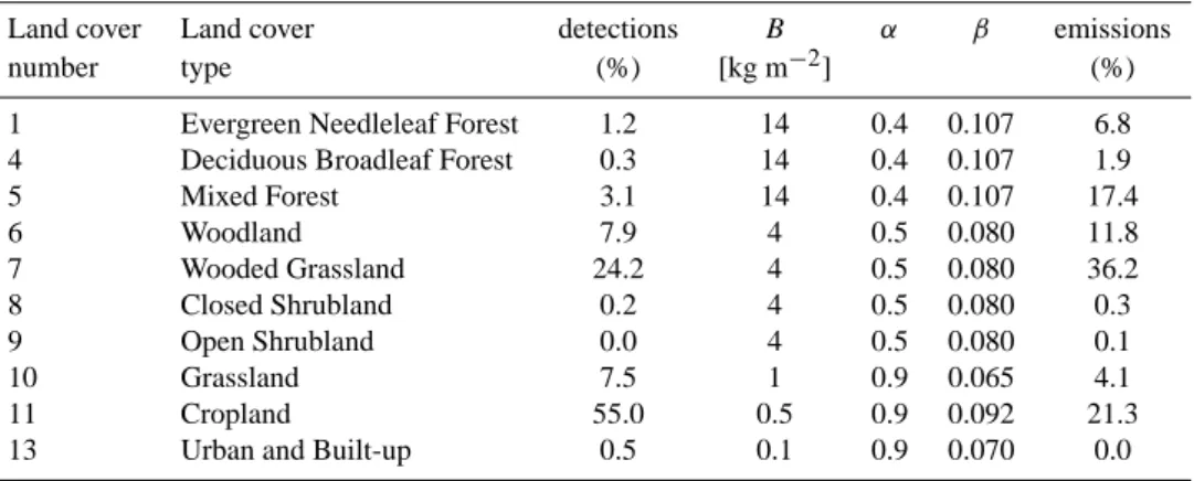
where A is the area burned, B is the biomass per area, α is the fraction of the biomass consumed by the fire, and β is the CO emission factor. Every detected fire was linked to a certain land cover type, using a global land cover classification with a resolution of 1 km (Hansen et al., 2000). Figure 5 shows a map of the MODIS fire detections between 21 April and 5 May as a function of land cover. The percentage of fires detected, the factors B, α and β used for the emission cal-culation, and the estimated emissions are reported in Table 1 for the various land cover types. The values of B and α are similar to those recently used by Wiedinmyer et al. (2006); values of β were taken from Andreae and Merlet (2001). The majority (55%) of the fires were detected in cropland, 24% in wooded grassland, 8% in woodland, 7% in grassland, and 5% in forests. Because of the low fuel loading in cropland, emissions there were only 21% of the total, whereas wooded grassland contributed 36%, woodland 12%, grassland 4%, and forests 26%.

It must be cautioned that our emission estimates are highly uncertain. We estimate that the total area burned is uncertain by at least a factor of two. We furthermore expect the attri-bution of fires to land cover types other than croplands to be biased high. In a pixel with a mosaic of different land cover types including croplands, a detected fire is most likely

burn-Table 1. Percentage of deteced fires, factors used for the emission calculations, and estimated CO emissions for the different land cover

classes from the Hansen et al. (2000) inventory. Only fires detected in the region north of 40◦N and between 20 and 60◦E, and during the period 21 April and 5 May, were considered here. Percentage values were normalized to the total number of detected fires, 7749, and the estimated total biomass burning emission, 1.6 Tg CO.

Land cover Land cover detections B α β emissions

number type (%) [kg m−2] (%)

1 Evergreen Needleleaf Forest 1.2 14 0.4 0.107 6.8 4 Deciduous Broadleaf Forest 0.3 14 0.4 0.107 1.9 5 Mixed Forest 3.1 14 0.4 0.107 17.4 6 Woodland 7.9 4 0.5 0.080 11.8 7 Wooded Grassland 24.2 4 0.5 0.080 36.2 8 Closed Shrubland 0.2 4 0.5 0.080 0.3 9 Open Shrubland 0.0 4 0.5 0.080 0.1 10 Grassland 7.5 1 0.9 0.065 4.1 11 Cropland 55.0 0.5 0.9 0.092 21.3

13 Urban and Built-up 0.5 0.1 0.9 0.070 0.0

Fig. 5. MODIS fire detections between 21 April and 5 May 2006.

The color indicates the dominant land cover where the detection oc-curred. Land cover classes 1, 4 and 5 from Table 1 were combined into “Forest”, classes 6-9 into “Mixed”.

ing on agricultural fields, since the fires were started by farm-ers. Our algorithm, however, attributes it to the dominant land cover type. Assuming that all fires actually burned on agricultural fields would lead to 60% lower total emissions. Additional uncertainties are associated with the factors B, α and β, such that the overall uncertainty of the BB emission estimate is at least a factor of three.

In addition to the BB emissions, we also used CO emis-sions from fossil fuel combustion (FFC) sources. For Eu-rope, we used the expert emissions taken from the UN-ECE/EMEP (United Nations Economic Commission for Europe/Co-operative Programme for Monitoring and Eval-uation of Long Range Transmission of Air Pollutants in Eu-rope) emission database for the year 2003. These data are based on official country reports with adjustments made by experts (Vestreng et al., 2005) and are available at 0.5◦ res-olution from http://www.emep.int. The emissions were uni-formly reduced by 10% to account for a likely reduction of

European CO emissions since 2003. Emissions elsewhere were taken from the EDGAR 3.2 Fast Track 2000 dataset (Olivier et al., 2001). Both datasets also include emissions from biofuel and waste burning, which were added to the FFC emissions.

5 Model simulations

Simulations of air pollution transport were made using the Lagrangian particle dispersion model FLEXPART (Stohl et al., 1998; Stohl and Thomson, 1999; Stohl et al., 2005) (see http://zardoz.nilu.no/∼_{andreas/flextra+flexpart.}

html). FLEXPART was validated with data from continental-scale tracer experiments (Stohl et al., 1998) and was used previously to study the transport of BB emissions to down-wind continents (Forster et al., 2001; Damoah et al., 2004) and into the Arctic (Stohl et al., 2006), as well as the trans-port of FFC emissions between continents (Stohl et al., 2003) and into the Arctic (Eckhardt et al., 2003). FLEXPART is a pure transport model and no removal processes were consid-ered here. The only purpose of the model simulations is to identify the sources of the measured pollution.

FLEXPART was driven with analyses from the European Centre for Medium-Range Weather Forecasts (ECMWF, 2002) with 1◦×1◦ resolution (derived from T319 spec-tral truncation) and two nests (108◦_W–27◦_{W, 9}◦_N–54◦_N;

27◦_W–54◦_{E, 35}◦_N–81◦_{N) with 0.36}◦_×0.36◦ _resolution

(derived from T799 spectral truncation). In addition to the analyses at 00:00, 06:00, 12:00 and 18:00 UTC, 3-hour fore-casts at 03:00, 09:00, 15:00 and 21:00 UTC were used. There are 23 ECMWF model levels below 3000 m, and 91 in to-tal. We also made alternative FLEXPART simulations us-ing input data from the National Centers for Environmental Prediction Global Forecast System (GFS) model with 1◦×1◦ resolution and 26 pressure levels.

-8 -8 0 0 8 8 8 8 8 8 8 8 8 8 8 8 8 8 16 16 16 16 16 16 16 16 16 16 16 24 24 24 24 20°N 20°N 40°N 60°N 80°N 180° 160°W 140°W 120°W 100°W 80°W 60°W 40°W 20°W 0° 20°E 40°E 60°E 80°E 100°E 120°E 140°E 160°E

ECMWF Analysis VT:Wednesday 3 May 2006 00UTC 1000hPa geopotential height

-8 -8 -8 -8 0 0 0 0 8 8 8 8 8 8 8 8 16 16 16 16 16 16 16 16 16 24 24 24 24 24 24 32 32 32 32 20°N 20°N 40°N 60°N 80°N 180° 160°W 140°W 120°W 100°W 80°W 60°W 40°W 20°W 0° 20°E 40°E 60°E 80°E 100°E 120°E 140°E 160°E

ECMWF Analysis VT:Wednesday 3 May 2006 00UTC 1000hPa temperature

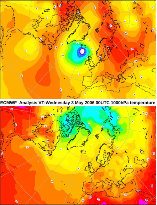
Fig. 6. ECMWF analyses of geopotential (top) and temperature (bottom) at the 1000 hPa level on 3 May 2006 at 00:00 UTC.

FLEXPART calculates the trajectories of so-called tracer particles using the mean winds interpolated from the analy-sis fields plus random motions representing turbulence. For moist convective transport, FLEXPART uses the scheme of Emanuel and ˇZivkovi´c-Rothman (1999), as described and tested by Forster et al. (2006). In order to maintain high ac-curacy of transport near the poles, FLEXPART advects parti-cles on a polar stereographic projection poleward of 75◦but using the ECMWF winds on the latitude-longitude grid to avoid unnecessary interpolation. A special feature of FLEX-PART is the possibility to run it backward in time (Stohl et al., 2003; Seibert and Frank, 2004).

For this study, FLEXPART was run both forward from the emission fields and backward in time from the Zeppelin sta-tion. The purpose of the forward simulation was to identify the areas affected by the BB emissions and to understand the transport in relation to the synoptic conditions. 13 million tracer particles of equal mass were released from the fire lo-cations, with the number of particles used depending on a fire’s calculated emission strength. The particles were in-jected between 0 and 100 m above the surface, as satellite images show that the agricultural fires did not trigger sub-stantial pyro-convection. Forward tracer simulations were also made for FFC CO emissions from Europe, North Amer-ica and Asia, respectively. Tracer particles were tracked for

20 days, after which they were removed from the simulation. Backward simulations from Zeppelin were made for 3-hour time intervals in April and May 2006. For each such interval, 40000 particles were released at the measurement point and followed backward in time for 20 days, forming what we call a retroplume, to calculate a potential emission sensitivity (PES) function, as described by Seibert and Frank (2004) and Stohl et al. (2003). The word “potential” indi-cates that this sensitivity is based on transport alone, ignor-ing removal processes that would reduce the sensitivity. The value of the PES function (in units of s kg−1) in a particu-lar grid cell is proportional to the particle residence time in that cell. It is a measure for the simulated mixing ratio at the receptor that a source of unit strength (1 kg s−1) in the respective grid cell would produce. For consistency with the forward simulations, we report PES values for a so-called footprint layer 0–100 m above ground. Folding (i.e., mul-tiplying) the PES footprint with the emission flux densities (in units of kg m−2_s−1_{) from the FFC and BB inventories}

yields so-called potential source contribution (PSC) maps, that is the geographical distribution of sources contributing to the simulated mixing ratio at the receptor. Spatial integra-tion finally gives the simulated mixing ratio at the receptor. Time series of these mixing ratios, obtained from the series of backward simulations, will be presented both for FFC and BB emissions. Since the backward model output was gen-erated daily, the timing of the contributing emissions is also known.

6 Pollution transport to the Arctic

The meteorological situation in the northern hemisphere in late April and beginning of May was characterized by so-called low-zonal-index conditions with large waves in the middle latitudes, which produced strong undulations of the jet stream and caused effective meridional exchange of air. This can be seen in Fig. 6 (top), which shows the situation on 3 May at 00:00 UTC, approximately at the time with the highest pollution levels measured at Spitsbergen. There were several strong high- and low-pressure centers in the north-ern hemisphere. The Icelandic low dominated the circula-tion over the northern North Atlantic and a prominent anti-cyclone was located over northeastern Europe. This pressure configuration corresponds to a positive phase of the North Atlantic Oscillation pattern, which is known to enhance pol-lution transport into the Arctic (Eckhardt et al., 2003). Con-sequently, air from the European continent was channelled into the Arctic between the two pressure centers, leading to abnormally high temperatures over the Norwegian and Bar-ents Seas and the Arctic Ocean (see Fig. 6, bottom). The situation on 25–27 April (not shown) was similar. Indeed, the first pulse of smoke arrived at Spitsbergen already on 27 April. Between the two episodes, the Icelandic low moved further north and interrupting the northward flow for two

days. This also brought some precipitation to Svalbard on 28 and 29 April (4 and 9 mm at Ny ˚Alesund). After 3 May, the anticyclone over Eastern Europe grew and extended fur-ther to the west. On 7 May, it stretched into the Norwegian Sea, such that air from Europe was first transported west-ward to the British Isles, and then around the high and to the north. Still later, the high’s center moved to Greenland, and the European outflow reached Iceland but not anymore Svalbard. While no precipitation was measured on Svalbard during the first days of May, the episode was ended by a cold front bringing rain and snow (1, 4 and 7 mm precipitation at Ny ˚Alesund on 6, 7, and 8 May) and finally clean Arctic air masses to the archipelago (Meteorological Institute, 2006).

The synoptic situation is somewhat reminiscent of the con-ditions when Arctic Haze is observed at Svalbard in win-ter and early spring (Iversen, 1984; Iversen and Joranger, 1985). However, instead of the pollution source region be-ing extremely cold as it occurs durbe-ing Arctic Haze, the Arc-tic receptor region became unusually warm in spring 2006. Should the warming of the Arctic continue to proceed more quickly than that of the middle latitudes, such transport con-ditions may become more frequent in the future.

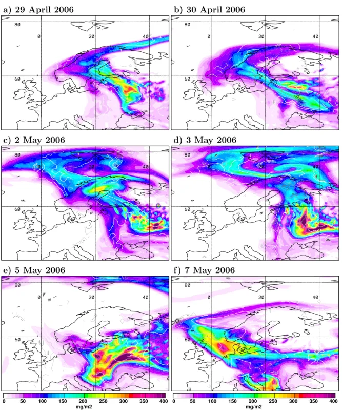
To illustrate the transport of the smoke from the fires in Eastern Europe, we show maps of the total column BB CO tracer from the FLEXPART forward simulation, with super-imposed MODIS AOD values, for the period 29 April–7 May (Fig. 7). AOD isolines are not closed where retrievals were not successful over snow-covered parts of Scandinavia, Arc-tic ice, and near clouds. We also compare the model results to CO retrievals from AIRS (Fig. 8). On 29 April (Fig. 7a), the plume stretched from the fire region where maximum AOD values were about 1.3 units, northwestward to Scandinavia. The close correspondence between the FLEXPART passive tracer simulation and the MODIS AOD field suggests that aerosols were not removed from the atmosphere to a signifi-cant extent, and that the aerosol distribution over Europe was dominated by the BB emissions. CO retrievals from AIRS (Fig. 8a) also show the highest values over the fire region but weaker spatial gradients.

One day later, on 30 April (Fig. 7b and 8b), the pol-lution plume reached the Norwegian Sea, and on 2 May (Fig. 7c and 8c), it had already arrived at Svalbard. AOD retrievals were not successful around Svalbard but values up to 1.5 units can be found a few degrees east of it (Fig. 7c). On 2 May, this plume is also the most prominent feature in the AIRS map (Fig. 8c). The retrieved CO enhancement over the Norwegian Sea (roughly 200 mg m−2_{above the background}

of about 1000 mg m−2_{) compares well with the FLEXPART}

BB CO tracer values in this region.

On 3 May, both the FLEXPART BB CO and AIRS CO show a dramatic increase over Eastern Europe, following the peak in the number of fire detections on 2 May. The roughly 400 mg m−2CO enhancement above the background seen by AIRS again agrees well with the FLEXPART BB CO in the fire region. The plume was still present around Spitsbergen

a) 29 April 2006

b) 30 April 2006

c) 2 May 2006

d) 3 May 2006

e) 5 May 2006

f) 7 May 2006

Fig. 7. Total columns of the FLEXPART biomass burning CO tracer at 09:00–12:00 UTC for (a) 29 April, (b) 30 April, (c) 2 May, (d) 3

May, (e) 5 May, and (f) 7 May 2006. Superimposed on the CO tracer maps are the 0.3, 0.5, 0.7, 1.0, 1.5, and 2 unit isolines (shown in white to dark gray) of the daily MODIS Terra Level-3 AOD product.

on 3 (Fig. 7d and 8d) and 4 May but then moved further to the northeast and was replaced by somewhat cleaner air on 5 and 6 May. On 5 May (Fig. 7e), a band of high AOD values (up to about 0.8 units) extended northwestwards from the British

Isles. This band is not associated with BB CO tracer but can be seen in the FFC CO tracer simulation (not shown) and, thus, can be attributed to the export of pollution from Western Europe. AOD maxima also occur southwest of Spitsbergen

a) 29 April 2006 b) 30 April 2006 0° 20° E 40° E 40° N 60° N 80° N 0° 20° E 40° E 40° N 60° N 80° N c) 2 May 2006 d) 3 May 2006 0° 20° E 40° E 40° N 60° N 80° N 0° 20° E 40° E 40° N 60° N 80° N e) 5 May 2006 f) 7 May 2006 CO Total Column (mg/m2) 500 700 900 1100 1300 1500+ 0° 20° E 40° E 40° N 60° N 80° N CO Total Column (mg/m2) 500 700 900 1100 1300 1500+ 0° 20° E 40° E 40° N 60° N 80° N

Fig. 8. Total CO columns retrieved from AIRS data for (a) 29 April, (b) 30 April, (c) 2 May, (d) 3 May, (e) 5 May, and (f) 7 May 2006.

(near 0◦W and 75◦N) where the FFC plume arrived on 6 May.

On 7 May (Fig. 7f), the BB plume was exported into the North Atlantic and arrived at Iceland on 8 May (not shown). This part of the plume did not reach Spitsbergen anymore where a change in wind direction replaced the polluted warm air with clean Arctic air (see the temperature drop in Fig. 1). Relatively high CO columns are still seen by AIRS over the Norwegian and Barents Sea on 5–7 May (Fig. 8e–f), which FLEXPART attributes mostly to FFC in Europe (not shown; but see Fig. 10, explained later).

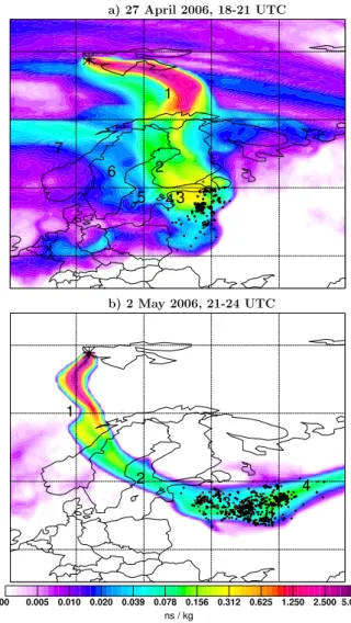
Figure 9 shows PES footprints of the retroplumes from the Zeppelin station for two 3-hour intervals, 27 April 18:00– 21:00 UTC and 2 May 21:00–24:00 UTC, during the two main observed pollution episodes. Fire detection locations are superimposed on the PES footprint maps in regions where and only for days on which the daily PES footprint value exceeds 0.005 ns kg−1 (nanoseconds per kilogram). For 27 April (Fig. 9a), the retroplume travels northward from Eastern Europe and converges towards the station from the east. The high PES footprint values (yellowish colors) ex-tend into the area where many fires were detected when the

air passed over it 3–4 days before its arrival at Zeppelin. For 2 May 21:00–24:00 UTC (Fig. 9b), the retroplume is more narrow and, in fact, the PES maps for 2, 3, and 4 May are all similar, with the retroplumes coming from Eastern Eu-rope and passing over Scandinavia. The air traveled over many fires 2–5 days before arriving at Zeppelin and picked up copious amounts of BB emissions. The air was also con-taminated with FFC emissions, mostly from around Moscow according to the PSC map (not shown). However, the total FFC CO is only 10 ppb, much less than the simulated BB CO of 72 ppb and the observed CO enhancement of about 100 ppb.

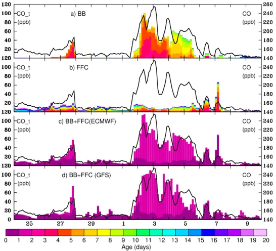
Figure 10 shows time series of the simulated CO tracer mixing ratios from all backward simulations between 24 April and 9 May. Simulated CO tracers are shown for BB (Fig. 10a) and FFC (Fig. 10b), BB+FFC (Fig. 10c), and BB+FFC obtained when using the alternative GFS analyses for driving FLEXPART (Fig. 10d). In all panels, the ob-served CO is shown as a black line. The previously high-est 2-hour mean CO mixing ratio measured at the station since the year 2001 of 230 ppb was exceeded on 2 and 3 May. Since simulated CO tracers accumulated emissions only over 20 days, they do not reproduce the observed CO background of about 140 ppb. However, the episodes of el-evated CO are well captured by the sum of BB and FFC CO tracers. There are subtle differences between the two sim-ulations using ECMWF and GFS data (e.g., the GFS simu-lation overestimates the CO peak on 27 April, whereas the ECMWF simulation overestimates the largely anthropogenic CO peak on 7 May) but generally both model versions re-produce the observed CO variations reasonably well. Both show a first pollution episode on 27 April, then a break, a strong episode from 1–5 May, followed by cleaner periods and weaker episodes on 6 and 7 May.

According to both model versions, BB emissions were always mixed with FFC emissions, which is not surprising given that the fires were burning in densely populated areas. There were some periods when FFC emissions dominated, e.g., on 6 and 7 May, but both model versions attribute most of the CO enhancement during the main episode from 1–5 May to BB. However, it is important to keep in mind that the relative contributions of FFC and BB emissions can be very different for species other than CO.

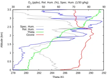
According to FLEXPART, the BB plume was traveling at altitudes below 3 km at all times. This is confirmed by plots of the corrected normalized relative backscatter signal from the micropulse lidar at Ny ˚Alesund (Fig. 11), which shows strong returns mostly below 2 km. On 2 May and on 3 May in the morning, when the highest pollution lev-els were measured at Zeppelin, the smoke aerosol concentra-tions decreased with altitude and the station was in the dens-est part of the plume. However, on 3 May in the afternoon, the smoke was more dense aloft. This is captured by the FLEXPART BB CO tracer simulation and also confirmed by an ozonesonde launched from Ny ˚Alesund on 3 May, which

a) 27 April 2006, 18-21 UTC

b) 2 May 2006, 21-24 UTC

Fig. 9. Potential emission sensitivity (PES) footprint maps for air arriving at Zeppelin on 27 April 2006, between 18:00 and 21:00 UTC (top), and for air arriving at Zeppelin on 2 May 2006, between 21:00 and 24:00 UTC (bottom). Black dots show MODIS fire detections on days when the footprint emission sensitivity in the corresponding grid cell on that day exceeded 0.005 ns kg−1. If a fire detection occurred in a pixel with forest as the main land cover type, a smaller red dot is superimposed. Numbers close to the main retroplume pathway label the plume centroid position at daily intervals.

shows increasing O3mixing ratios up to 2 km and a decrease

at about 2.4 km (see Fig. 15, discussed later). On average, the smoke observed at Ny ˚Alesund had a layer thickness of about 2 km and, thus, filled a significant part of the troposphere.

7 Air chemistry and aerosol observations

7.1 Halocarbons

The hydrofluorocarbons HFC-134a and HFC-152a (atmo-spheric lifetimes of 14 and 1.4 years, respectively) are used

Fig. 10. Comparison of time series of modeled CO tracers from the backward simulations (colored bars, referring to left axes) with measured

CO (black lines, referring to right axes) at Zeppelin. Measured CO is shown in every panel, whereas the colored bars are (a) biomass burning (BB) CO tracer, (b) fossil fuel combustion (FFC) CO tracer, (c) BB+FFC CO tracer, (d) BB+FFC CO tracer. Model results shown in panels (a–c) were produced by driving FLEXPART with ECMWF analyses, whereas those shown in panel (d) were produced with GFS data. The colors in (a) and (b) give the age (i.e., time since emission) of the CO tracers according to the label bar, whereas in (c) and (d) the colors separate FFC (darker color) and BB CO (lighter color).

Fig. 11. Normalized relative backscatter (NRB), corrected for Rayleigh contribution, from the micropulse lidar located at Ny ˚Alesund measured during the period 26 April to 9 May 2006. White areas correspond to missing data. Two periods (28 April–1 May, 5–7 May) are not shown because of poor data coverage due to the presence of clouds.

as refrigerants and blowing agents for producing insolation foams (WMO, 2005). Since they have no natural sources, they are excellent tracers for emissions from anthropogenic activities. At remote observatories, distinct peaks of

HFC-134a and HFC-152a concentrations occur when air masses from major population centers are transported to the station (Reimann et al., 2004). Even though 134a and HFC-152a are not themselves emitted by FFC, their regional

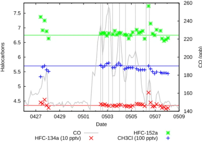
4.5 5 5.5 6 6.5 7 7.5 0427 0429 0501 0503 0505 0507 0509 140 160 180 200 220 240 260 Halocarbons CO (ppb) Date CO HFC-134a (10 pptv) HFC-152a CH3Cl (100 pptv)

Fig. 12. Time series of measured CO, HFC-152a, HFC-134a, and

CH₃Cl measured at Zeppelin from 26 April to 9 May 2006. Hor-izontal lines, as well as vertical lines through local CO maximum and minimum values are drawn for better guidance.

sion patterns correlate with those of FFC, such that they can help identifying when pollution levels are influenced by FFC emissions. In contrast, methyl chloride (CH3Cl) has mostly

natural sources, including BB (Khalil and Rasmussen, 1999, 2003).

Figure 12 shows HFC-134a, HFC-152a, and CH3Cl

mea-surements superimposed on the time series of measured CO. Instrument maintenance work was performed at the end of April/beginning of May, such that the data record is unfortu-nately not complete but still sufficient for our purpose. The anthropogenic tracers HFC-134a and HFC-152a both have their highest values on 27 April and 6 May, at times when FLEXPART suggests relatively strong FFC episodes (see Fig. 10). The enhancements during the main CO episode from 1–5 May are much smaller. HFC-134a values are higher at the beginning (2 May) and at the end (5 May) of this period than in its middle (3–4 May), in agreement with the FLEXPART FFC CO tracer concentrations (Fig. 10). On the other hand, CH3Cl is well correlated with CO in the BB

plume. The peak enhancement above the background on 3 May of about 30 pptv corresponds to an enhancement ratio (ER) of 0.0003, relative to the 100 ppb CO enhancement. This is consistent with reported CH3Cl/CO emission ratios

from vegetation fires (Andreae and Merlet, 2001). In sum-mary, this confirms that at Zeppelin CO was dominated by BB emissions, whereas FFC emissions played a smaller role. 7.2 Carbon dioxide

Figure 13 compares time series of CO2 and CO. The

two species co-variate from 24 April-5 May but are anti-correlated later on. The likely reason for the anti-correlation during the FFC episodes on 6 and 7 May is that the source regions for these episodes are in Western Europe where the

383 384 385 386 387 388 389 390 0425 0427 0429 0501 0503 0505 0507 0509 140 160 180 200 220 240 260 CO2 (ppm) CO (ppb) Date CO CO₂

Fig. 13. Time series of CO2and CO measured at Zeppelin from 24

April to 10 May 2006.

vegetation was already active and took up more CO2 than

what was emitted by FFC. However, during the major BB episode, CO and CO2are highly correlated, thus facilitating

a regression analysis. Since CO data were available as two-hour means with irregular starting times, every CO value was assigned the 1-hourly CO2value that fell entirely into the CO

sampling interval. Standard linear regression analysis with CO2as the independent variable resulted in a CO/CO2slope

of 0.023 (after conversion to mass mixing ratios) and a Pear-son correlation coefficient of 0.91 for the period 1–4 May. In comparison, average CO/CO2emission ratios from

pas-senger cars range from 0.002–0.016 (Vasic and Weilenmann, 2006) and, according to the EDGAR inventory, Germany’s overall CO/CO2emission ratio in the year 2000 was about

0.006. Agricultural fires have a much higher CO/CO2

emis-sion ratio of 0.06 with an uncertainty of a factor of two (An-dreae and Merlet, 2001). Assuming CO/CO2emission ratios

of 0.006 and 0.06 for FFC and BB emissions, respectively, the observed CO/CO2 slope of 0.023 indicates that 35% of

the CO2and 82% of the CO variability during 1–4 May were

due to BB. 7.3 Ozone

The peak O3mixing ratios during both episodes clearly

ex-ceeded the previously set long-term (since 1989) record-high 1-hour-mean mixing ratio of 61 ppb at the Zeppelin station and set a new record of 83 ppb (Fig. 14). An ozonesonde launched on 3 May at 11:00 UTC measured increasing O3

mixing ratios with altitude up to some 2400 m asl, above which O3decreased sharply at a temperature inversion that

capped the polluted layer (Fig. 15).

In order to explore whether the extremely high O3

lev-els were due only to the high loads of precursor substances or also to especially effective O3 formation, we performed

0 10 20 30 40 50 60 70 80 90 0425 0427 0429 0501 0503 0505 0507 0509 140 160 180 200 220 240 260 Ozone (ppb), GEM (30 pg/m3) CO (ppb) Date I II III OS* CO Hg O₃

Fig. 14. Time series of CO, O3, and GEM measured at Zeppelin

from 24 April to 10 May 2006. Vertical lines mark the duration of periods ”I”, ”II” and ”III”, respectively. The asterisk labelled “OS” indicates the launch time of an ozonesonde from Ny ˚Alesund.

0 0.5 1 1.5 2 2.5 3 3.5 278 280 282 284 286 288 290 292 30 40 50 60 70 80 90 Altitude (km) Theta (K)

O₃ (ppbv), Rel. Hum. (%), Spec. Hum. (1/30 g/kg)

Spec. Hum. Rel. Hum. Theta Ozone

Fig. 15. Vertical profiles of specific humidity, relative humidity,

potential temperature (Theta), and O3obtained from an ozonesonde

launched at 11:00 UTC on 3 May from Ny ˚Alesund.

independent variable, for the three periods marked in Fig. 14, and for the remaining April-May data. As described be-fore for CO2, every 2-hourly CO value was assigned a

1-hourly O3value. Figure 16 shows a scatter plot of O3versus

CO data for the different time periods, with regression lines drawn through the data, and Table 2 reports the regression parameters. Overall, there is a positive O3-CO correlation in

April-May 2006, which is indicative of a regime dominated by photochemical O3formation. Note that a negative O3-CO

correlation would be expected for air masses originating in the stratosphere but stratospheric air masses cannot normally descend into the Arctic polar dome (Stohl, 2006). Pearson correlation coefficients for the three periods range from 0.84– 0.87, indicating compact positive O3-CO relationships.

Table 2. Analyses of the correlations between CO and O3at

Zep-pelin for different periods as defined in Fig. 14. Shown are the number of data points (N ), the Pearson correlation coefficient (r), the slope, and the intercept of the regression line. For the second pe-riod, calculations were also performed separately for CO≤200 ppb, and CO>200 ppb, respectively.

Period N r slope intercept Period I 19 0.87 0.53 −26.7 ppb Period II 64 0.84 0.34 1.6 ppb Period II, CO ≤200 ppb 39 0.85 0.51 −28.3 ppb Period II, CO >200 ppb 25 0.23 0.04 67.6 ppb Period III 15 0.87 0.58 −36.2 ppb Rest of April-May 614 0.61 0.42 −22.6 ppb

The slopes of the O3-CO regression lines are of particular

interest, since they inform about the number of O3molecules

formed per CO molecule emitted, assuming that both CO and O3are conserved during transport. For aged North American

FFC plumes in the North Atlantic region in summer, Parrish et al. (1998) reported average O3-CO slopes of 0.25–0.40,

with values up to 1.0 for individual plumes. For the Azores, an average slope of 1.0 was reported for summer conditions (Honrath et al., 2004). For aged BB plumes, O3-CO slopes

are normally less steep, which is due to the lower NOx/CO

emission ratios of BB compared to FFC and, thus, less effi-cient O3formation per CO molecule. Over Alaska, Wofsy et

al. (1992) found average O3-CO slopes of 0.1 in BB plumes;

downwind of North American boreal forest fires, Real et al. (2006) reported small negative to small positive values; Wotawa and Trainer (2000) found small positive slopes of 0.05–0.11 in BB plumes transported from Canada to the east-ern United States; for the Azores, Honrath et al. (2004) re-ported a range of 0.4–0.9 for plumes from boreal forest fires (with contributions from FFC); and Andreae et al. (1994) re-ported slopes of 0.46±0.23 for BB plumes over the tropical South Atlantic.

The O3-CO slope of 0.42 found for our data set for the

non-episode periods in April–May (Table 2) lies between the slopes of 0.25–0.40 reported by Parrish et al. (1998) and 1.0 by Honrath et al. (2004) for FFC combustion plumes in sum-mer. The slopes for BB period I (0.53) and (mostly) FFC combustion period III (0.58) are large compared to previ-ously reported values, indicating highly efficient O3

forma-tion. The slope for BB period II is lower (0.34) but this is a result of a curvature in the O3-CO correlation. Separate

re-gression analyses for CO mixing ratios below 200 ppb CO (slope of 0.51) and above 200 ppb CO (slope of 0.04) indi-cate that for the lower CO mixing ratios, the slope is similar to BB period I. The lack of correlation between O3and CO

at the higher CO levels indicates less efficient O3formation

in those air masses that have received the largest CO (and likely also NOx) input. In addition, model calculations by

10 20 30 40 50 60 70 80 90 100 140 160 180 200 220 240 260 O3 (ppb) CO (ppb) Rest Episode 2 Episode 3 Episode 1

Fig. 16. Scatter plot of O3versus CO data from Zeppelin. The

data points are colored according to the three periods defined in Fig. 14, and the rest of the data for April–May 2006 is shown in grey. Regression lines through the various data sets are also shown in corresponding colors.

Real et al. (2006) showed that the strong aerosol light extinc-tion in dense BB smoke plumes can decrease O3formation

efficiency.

Despite the decrease in O3 formation efficiency at the

highest CO levels, the O3-CO slopes are higher than most

values reported in the literature for BB plumes. This is dif-ficult to explain since these events took place at high lati-tudes and early in the year. Photolysis rates for these air masses were certainly not optimal for ozone production. Fur-ther, preliminary model simulations with the EMEP MSC-W model (Simpson et al., 2003) have failed to simulate the ob-served ozone increase, despite predicting reasonable values of CO, sulphate and nitrate. It is therefore not entirely clear why the O3-CO slopes are so large, and further model

simu-lations will be needed to quantify the underlying processes. However, several factors could have enhanced the O3

forma-tion: Firstly, FFC emissions of NOxwere not negligible and

were mixed into the BB plumes, which would have shifted the O3-CO slope towards the higher values typical for FFC

plumes. Furthermore, the agricultural areas in Eastern Eu-rope receive large nitrogen loads from fertilization but also from atmospheric deposition. NOxemissions from the fires

can be unusually high in such conditions (Hegg et al., 1987), and microbial NOx emissions from the soils (Stohl et al.,

1996) may have been significant, too. Secondly, no clouds were present and the plumes crossed snow-covered regions whose high albedo enhanced the available radiation. Thirdly, a stable stratification of the polluted air mass is likely along most of the trajectory, as the warm air from continental rope passes over the snow-covered regions of northern Eu-rope and the relatively cold Atlantic (see, e.g., Fig. 15 for conditions at Ny ˚Alesund). This stable stratification, as well as the nature of the surface, would ensure very low deposition

10 20 30 40 50 60 70 80 90 01 02 03 04 05 40 50 60 70 80 90 0501 0503 0505 0507 0509 0511 0513 Ozone (ppb) Date

Fig. 17. Time series of O3measured at Storhofdi on Westman

Is-lands, Iceland, for the period 1 to 13 May. The inset shows the O3

time series for the first five months of the year 2006. The event clearly stands out from the normally rather constant background.

of ozone and other gases over a large fraction of the transport distance. Fourthly, due to the delayed onset of spring in Eu-rope, the vegetation was still dormant, which might have also reduced the dry deposition of O3.

High O3concentrations similar to those measured at

Zep-pelin were monitored at several other stations in northern Scandinavia, as the smoke plume was transported across (not shown). Figure 7f shows that the plume also approached Ice-land on 7 May. One day later it arrived at the measurement site at Storhofdi and produced strongly elevated O3 values

for about three days (Fig. 17). Normally, O3at Storhofdi is

rather constant at between 40 and 50 ppb in winter and spring (see inset in Fig. 17) and 30 ppb in summer. In fact, in the past O3levels have exceeded 70 ppb only on three other

oc-casions during the periods with available data (1992–1997, 2003–present). The peak hourly O3mixing ratio of 88 ppb

measured during the smoke event is 13 ppb higher than any previously measured event.

7.4 Gaseous elemental mercury

Gaseous elemental mercury (GEM) was elevated but not well correlated with CO during the BB episodes (Fig. 14). Mea-surements of GEM in BB plumes are rare but the following ER to CO have been reported: 0.067×10−6_{ppb GEM/ppb}

CO (Friedli et al., 2003a) for a mixture of conifers, grass and shrubs, 0.204×10−6_{ppb GEM/ppb CO (Friedli et al., 2003b)}

for black spruce, 0.21×10−6ppb GEM/ppb CO (Brunke et al., 2001) for fynbos, and 0.086×10−6ppb GEM/ppb CO (Sigler et al., 2003) for black spruce and jack pine. Assuming the highest reported ER of 0.21×10−6ppb GEM/ppb CO, the observed maximum CO enhancement at Zeppelin of 100 ppb would correspond to 182 pg m−3GEM enhancement. How-ever, observed GEM increased by more than 600 pg m−3.

A p r 1 A p r 5 A p r 9 A p r 1 3 A p r 1 7 A p r 2 1 A p r 2 5 A p r 2 9 M a y 3 M a y 7 M a y 1 1 M a y 1 5 M a y 1 9 M a y 2 3 M a y 2 7 M a y 3 1 0 500 1000 1500 2000 2500 3000 3500 4000 N 1 0 0 ( cm -3 ) Date Observation 2006 Median (2000-2005) 95%-tile (2000-2005)

Fig. 18. Time series of the daily mean number concentrations of

ac-cumulation mode (100–500 nm diameter) particles at Zeppelin for the period April–May 2006. The horizontal lines show the median and the 95-percentile obtained for the months of April and May in the years 2000–2005. Days for which aerosol size distributions are shown in Fig. 19 are marked with circles.

This, and the lack of correlation with CO suggests that GEM was mostly not coming from BB. Nevertheless, the measured GEM levels are among the highest ever measured during a transport event. Normally, such high levels are reached only during short periods, typically following re-emission of GEM from the ground, after mercury depletion events. 7.5 Aerosol mass and size distribution

Regarding the aerosol physical properties, the DMPS mea-surements revealed that the key characteristic of the BB episodes is the numerous accumulation mode particles. Fig-ure 18 compares the median and 95-percentile of daily mean particle number densities between 100 and 500 nm diame-ter calculated for April and May of the years 2000 to 2005 (85% data coverage) with the observations from 2006. The BB plume events are associated with number concentrations about 10 times larger than the 95-percentile, but the whole period shows a tendency of elevated accumulation mode par-ticles.

To illustrate the enhanced accumulation mode, we have selected six days from just before, during and after the BB episode (marked with circles in Fig. 18). Of these six days, two days represent median accumulation mode number den-sities, two represent the 95-percentile, and two represent the plume peaks during the events, respectively. Figure 19 compares the aerosol size distributions for these six days. The difference between the pre- and post-episode median and 95-percentile distributions are that the May distributions present a broader accumulation mode and a reminiscence of

0.1 10 1 10 2 10 3 d N/d l o g Dp ( cm -3 ) Dp (µm) 2006-04-20 2006-04-21 2006-04-27 2006-05-02 2006-05-14 2006-05-16

Fig. 19. Aerosol number size distributions measured at Zeppelin on

selected days in April and May 2006 as shown in Fig. 18.

an Aitken mode. This is rather typical for the site (Str¨om et al., 2003) as cloud processing and new particle formation within the Arctic become dominating processes during later May and early June. The plume events are characterized with the complete absence of an Aitken mode, an increase in the number of accumulation mode particles, and a shift towards larger sizes. The later suggests a large increase in particle mass.

Particle mass (PM) concentrations are not measured di-rectly at Zeppelin but they can be estimated from two in-dependent data sets. Firstly, daily means of PM were esti-mated from the DMPS aerosol number concentration mea-surements, assuming a density of the aerosols of 1.5 g cm−3. Since information on particles larger than 0.7 µm was miss-ing, this approach provides a conservative estimate of the PM concentrations encountered during the event. Secondly, we can derive PM from available nephelometer observations (not shown here) using the mean mass scattering coefficient of 1.1 m2g−1reported by Adam et al. (2004) observed in a forest fire plume over the northeastern USA. Since the mass scattering coefficient varies with the type of aerosols encoun-tered, the second approach must be considered highly uncer-tain. Nevertheless, the resulting two PM data sets are closely correlated with a correlation coefficient above 0.98, with the nephelometer-based estimates being higher by almost a fac-tor 2. The DMPS approach provided a maximum 24 h PM concentration of 29 µg m−3during the BB event, which cor-responds to an increase by more than an order of magnitude from conditions before and after the episode (Fig. 20). PM concentrations are also closely correlated with CO.

0 0.1 0.2 0.3 0.4 0.5 0.6 0.7 0.8 0.9 0425 0427 0429 0501 0503 0505 0507 0509 140 160 180 200 220 240 260

EBC, EC (ug/m3), OC (10 ug/m3), PM (100 ug/m3)

CO (ppb) Date CO EC OC PM EBC

Fig. 20. Time series of equivalent black carbon (EBC) and CO

mea-sured at Zeppelin from 24 April to 10 May 2006. Also shown are el-emental carbon (EC) and organic carbon (OC) concentrations from weekly samples and daily mean particle mass (PM) concentrations derived from the DMPS data.

7.6 Carbonaceous material

The time series of EBC measured with the PSAP and CO are highly correlated, especially during the BB episode (Fig. 20). For period II, as defined in Fig. 14, their correlation coeffi-cient is 0.91 and, after conversion of CO mixing ratios to concentrations, the EBC/CO slope of the regression line is 0.007. This is almost exactly the mean EBC/CO emission ratio, 0.0075, reported for agricultural burning by Andreae and Merlet (2001).

Concentrations of EC and OC (together comprising to-tal carbon, TC) from weekly filter samples are also shown in Fig. 20. There is generally good agreement between the EBC measured with the PSAP and the EC measured with the thermo-optical method. For the sample covering the main BB period from 30 April–7 May, EC and corresponding aver-age EBC concentrations are 0.24 µg m−3and 0.28 µg m−3, respectively.

A very low EC/TC ratio of 0.06 was observed during the BB event, which is considerably lower than what has been re-ported previously for emissions from burning of agricultural waste (e.g., 0.17 by Andreae and Merlet, 2001). It could be speculated that this is due to condensation of secondary organic material during transport. Furthermore, pollen was observed in the BB plume as it was transported across Scan-dinavia. If some of this pollen was transported further to Spitsbergen, it would have contributed to the very high OC fraction. For the proceeding weeks of the BB event, the EC/TC ratio ranged from 0.19–0.39, indicating contribution from sources more rich in EC.

The EC/EBC concentrations measured during the BB episode are extremely high for an Arctic station. The highest 1-hour mean EBC concentration measured at

0 0.2 0.4 0.6 0.8 1 1.2 0425 0427 0429 0501 0503 0505 0507 0509 0 0.5 1 1.5 2 2.5 3 3.5

SO4-S, NO3-N (ug/m3)

K (100 ng/m3), Levoglucosan (ng/m3) Date CO (relative units) SO4-S NO3-N K Levoglucosan

Fig. 21. Time series of CO, and NO−₃-N, SO2−₄ -S and K+from daily, and levoglucosan from irregular filter samples taken at Zep-pelin.

pelin during the period November 2002-August 2005 was 0.28 µg m−3, the same value as reported above for the weekly mean and a third of the highest hourly value mea-sured during the BB episode (0.85 µg m−3_{). Thus, the BB}

episode clearly exceeded any Arctic Haze event observed at Zeppelin in these years. An even higher hourly EBC value of 3.4 µg m−3was measured at Barrow, Alaska when a boreal forest fire plume reached the site (Stohl et al., 2006). How-ever, these fires were burning closer to the station than in our case.

7.7 Aerosol chemical composition

Levoglucosan is a specific tracer for BB, which is mostly associated with the fine fraction of aerosols and emitted in sufficiently large quantities to be detectable far away from the fire location (Simoneit et al., 1999). Potassium is an-other tracer for BB emissions, particularly for those occur-ring under flaming conditions (Echalar et al., 1995) but is less specific than levoglucosan as it also has other sources. Both levoglucosan and potassium were measured on aerosol filter samples from Zeppelin and both show greatly elevated concentrations during the episodes on 27 April and 1–5 May (Fig. 21). For the highest measured values, the ER values of potassium and levoglucosan relative to CO were about 0.0026 and 0.000047, respectively. The potassium/CO ER is in the middle of the range given for the emission ratio by An-dreae and Merlet (2001), while the levoglucosan/CO ER is more than an order of magnitude lower than what measured levoglucosan emission factors from agricultural BB (Hays et al., 2005) would suggest. Since aerosols do not seem to have been removed to any significant extent, we suggest that degradation of levoglucosan during transport is a possible reason for the relatively low levoglucosan/CO ER. In a re-cent laboratory study by Holmes and Petrucci (2006), it was suggested that levoglucosan could be subjected to

0 10 20 30 40 50 60

23-30 April 30/4-7/5 7-14 May 14-21 May 21-27 May

Relative contribution (%) EM OM SIA SS Pot.+Calc.

Fig. 22. Relative contributions of different chemical compound

classes as defined in the main text, to the total speciated aerosol mass at Zeppelin for the weeks 17–21 of the year 2006.

ization in the atmosphere.

There also exists a long-term record of potassium mea-surements at Zeppelin. For the years 1993–2003, we found twelve values greater than the highest value measured on 2–3 May 2006 (0.26 µg m−3). Thus, such extreme BB episodes are infrequent at Zeppelin, but occasional episodes may have occurred before.

Sulfate and nitrate were also elevated in the BB plume, reaching 1.2 µg S m−3 (0.12 µg S m−3 of which are at-tributable to sea salt) and 0.71 µg N m−3, respectively, in the sample taken on 2 May. Again, few (8 for sulfate, 11 for nitrate) higher values were found in the long-term (1993– 2003) dataset. In addition, gas-phase SO2 and HNO3

con-tributed 0.4 µg S m−3 and 0.13 µg N m−3, respectively. Note that while the sum of aerosol nitrate and HNO3is

mea-sured accurately, their separation is uncertain with the em-ployed method. Average FLEXPART FFC source contribu-tions on that day of 1.5 µg S m−3and 1.1 µg N m−3suggest that the FFC emissions may suffice for explaining the added gas- and aerosol-phase sulfur and nitrogen concentrations if no removal took place en route. However, FLEXPART pre-dicts several episodes every year with similar or higher FFC source contributions but without observations reaching such high levels, indicating that removal processes are normally more effective than in the BB plume. Furthermore, using an average emission ratio of NOx-N/CO of 0.013 for

agricul-tural BB (Andreae and Merlet, 2001) and the observed mean CO enhancement of about 100 µg m−3_{would give}

approx-imately 1.3 µg N m−3 from BB, more than the FFC con-tribution. Soil NOx emissions may have contributed, too.

Reported emission factors for SO2 from BB are lower but

may not be appropriate because the fires burned in a region that received large deposition loads of sulfate from FFC in the past decades (Mylona, 1996). Re-emission of deposited sulfur by fires was recently suggested as an important

0 0.1 0.2 0.3 0.4 0.5 0.6 0.7 0425 0427 0429 0501 0503 0505 0507 0509 0 20 40 60 80 100 120 140 160 AOD at 500 nm BB CO tracer column (mg/m2) Date

Fig. 23. Time series of aerosol optical depth (AOD) measured at

500 nm (symbols) and total columns of the FLEXPART biomass burning (BB) CO tracer (line) at Ny ˚Alesund from 24 April to 10 May 2006.

anism (Langmann and Graf, 2003). Thus, it is quite likely that even for sulfate and nitrate, BB emissions made a sig-nificant contribution to measured values on 2–3 May. This would also allow for some deposition to have occurred.

To study how the BB event affected the aerosol chem-ical composition relative to conditions before and after and to summarize our data, we performed a chemical mass balance calculation. The time resolution of the cal-culation was limited to one week by the EC/OC data, and since these measurements were started only a week before the event, results for only five weeks are pre-sented. The mass balance comprises contributions of organic matter (OM=OC×1.8), EM (EM=EC×1.1), sec-ondary inorganic aerosols (SIA=SO2−₄ +NO−₃+NH+₄), sea salt (SS=Na++Cl−+Mg2+), and the sum of K+ and Ca2+. The total speciated mass concentrations exceeded the PM con-centrations derived from the DMPS measurements by 10– 60%, except for the sample from 30 April to 7 May when the DMPS value is higher by about 10%. The fact that the total of the speciated mass concentrations is higher than the DMPS estimate, is to be expected because aerosols greater than 0.7 µm are not accounted for in the latter. In Fig. 22, the increased relative contribution of organic matter during the event is striking. While organic matter accounted for 59% of the sum of the speciated mass during the BB event in the first week of May, the corresponding percentage for the pro-ceeding weeks ranged from 4–9% only. In contrast, sea salt accounted for only 9% during the event but between 23 and 50% in the proceeding weeks.

7.8 Aerosol optical depth

Figure 23 compares the AOD at 500 nm measured at Ny ˚